Mar 6, 2007 - Finding a feasible solution to this problem with CPLEX 9.0 took about 70 seconds on IBM Thinkpad. T42 with a 1.8Ghz Pentium processor.
Mixed integer-linear formulations of cumulative scheduling constraints A comparative study Martin Aronsson, Markus Bohlin, Per Kreuger Swedish Institute of Computer Science email:{martin.aronsson,markus.bohlin,per.kreuger}@sics.se
2007-03-06 SICS Technical Report T2007:03 Abstract This paper introduces two MILP models for the cumulative scheduling constraint and associated pre-processing filters. We compare standard solver performance for these models on three sets of problems and for two of them, where tasks have unitary resource consumption, we also compare them with two models based on a geometric placement constraint. In the experiments, the solver performance of one of the cumulative models, is clearly the best and is also shown to scale very well for a large scale industrial transportation scheduling problem.
Keywords Cumulative scheduling, MILP modelling and pre-processing, railway transport scheduling
ISSN 1100-3154 ISRN: SICS-T–2006/02-SE
1
Introduction
Constraint programming (CP) techniques have been quite successful in solving both academic [9, 2, 11, 8, 3] and real-world scheduling problems [14, 13, 15, 16, 7]. One of the main benefits of CP for such problems is the presence, in most modern solvers, of very efficient filtering mechanisms in the form of constraint abstractions for both classical job shop and generalisations such as the cumulative resource scheduling problem. Using demand-driven filtering during search for integer solutions constitutes a powerful decision mechanism that can even be used successfully for optimisation [10, 11]. To optimise classical job shop problems and their cumulative generalisations efficiently it is generally also necessary to employ quite sophisticated search heuristics. Mixed Integer Linear Programming (MILP) is another technique for combinatorial problem solving which has been applied to a wide variety of industrial-level problems. For scheduling problems with single activity resources, standard linear boolean formulations also scale very well, especially for problems with a lot of linear side conditions that can be exploited by modern MILP solvers. For cumulative scheduling problems, however, there does not seem to exist any standard MILP formulations. For certain classes of problems, e.g. where all tasks have unitary resource consumption, formulations based on geometric placement can be used [21]. These can, as we will see, be quite efficient for the problems they can encode. Cumulative constraints [1] are well known in the CP community where efficient algorithms based on sweep [6] and/or task-intervals [12] are used to prune the search space, both as a pre-processing mechanism and on demand for variable domain reduction during search. Several variants of the constraint has been described e.g. in [5]. These constraints normally restrict the cumulative capacity utilisation of tasks executing simultaneously not to exceed a fixed capacity. Capacities and capacity utilisation are normally fixed integers and the start times and durations, decision variables. Variants where the resource consumption of each task is also variable and possibly constrained by the start time and duration occur as well. In this paper we focus on the case where the capacity and the resource consumption are constant integers. We have not found this to be restrictive in practice for problem domains we have considered. Geometric placement constraints are related to cumulative constraints. The most common form is probably that of filtering for non-overlap of rectangles in the plane [4] which, in the context of scheduling, corresponds to allocation of unit capacity resources to tasks with unit resource consumption combined with a multi-resource scheduling problem. The resource allocation is represented as the placement of a a unit height rectangle in the y-dimension and the start time as the placement of its left edge and the duration as its length in the x-dimension. In classical cumulative scheduling, there is no concept corresponding to the placement of the lower edge on the y-axis, and the resource consumption is arbitrary. Still, the special case of unit resource consumption is of considerable practical interest, and for these, the placement formulation can be used by considering the number of resources as a cumulative capacity and just ignoring the values the yplacement variables. Any solution to the placement problem is clearly feasible for the cumulative as well. That any solution satisfying the cumulative can also be realised as a placement is true for the case where heights are one but not in general. We will, after some preliminaries, describe four different models, two for the placement formulation and two for the the cumulative constraint, define filtering methods for each, note some of their complexity properties and investigate their solving performance on three separate sets of problems. The first two set of problems are derived from a practical case in rail traffic scheduling where all the tasks have unit resource consumption. In the third, a set of random problems with a more general structure and of varying sizes and difficulties are studied. In addition, in a fourth empirical section, we briefly describe the results of using a selection of the described methods in an industrial scale rail transport scheduling problem. This problem was what originally motivated our research, and even though the problem has a quite special structure it is of great practical importance. We conclude with a summary of our findings.
2 2.1
Preliminaries and notation Notation for model parameters and variables
Let n denote the number of tasks in the problem and use 0 < i, j ≤ n as task indexes. Let, furthermore, c denote the resource capacity limit and hi the resource consumption for task i. Let si denote the start
2
time variable for task i, bounded by an interval si ≤ si ≤ si and di the duration variable for task i, bounded by an interval di ≤ di ≤ di .
2.2
Maximal clique construction
In cumulative scheduling it is often useful to do an analysis of the parameters and bounds of the problem. One of the most obvious ways to do this is to construct subsets of tasks that can overlap in time. In CP, this type of computation is performed iteratively during search to filter the domains or bounds of the decision variables, but it can also be used for pre-processing in MILP formulations to filter equations and booleans that need not be maintained by the solver. Formally, this is achieved by considering the tasks of the problem as nodes in a graph and letting two tasks i and j, be connected by a link if and only if they can overlap in time, i.e. if either si ≤ sj < si + di or sj ≤ si < sj + dj . Then, all maximal cliques (completely connected sub-graphs) of this graph will have the property that, unless a task is already in the clique, it cannot overlap all the others. This is a very useful property in cumulative scheduling since when we wish to limit the number of simultaneously overlapping task, it is sufficient to consider each maximal clique separately. The complexity of enforcing cumulative conditions on the set of all tasks is often bounded by some function of the sizes of the maximal cliques, rather than the size of the task set itself. In practical problems this is often of great value, since the majority of tasks cannot be arbitrarily placed in time. This makes the maximal cliques small compared to the total number of tasks. Note also that many tasks may appear in several maximal cliques. Therefore it makes sense to check that equations (and booleans) relating pairs of tasks in one clique are not reproduced when analysing another clique which happen to contain the same two tasks. To construct the set of all maximal cliques used in the models below, we use a straightforward sweep algorithm which has linear time complexity in the size of the set of tasks. In the model description below we will often generate a set of equations for each maximal clique Clqk and where 1 ≤ nk ≤ n is the size of the k’th clique.
3
Model descriptions
The first two models described below are restricted to handle tasks with unitary resource requirements. The reason for this is that these are based on a rectangle placement approach which does not capture the general cumulative case. They are, in fact, more close to ones for placing non-overlapping rectangles of unit height onto the plane. In practice however, these are quite useful models since in many situations where the cumulative constraint is used, there is an underlying problem structure of this type. E.g. in train scheduling, a station may be modelled as a cumulative resource that allows a maximum number of trains to occupy the station at any one time. The type of model proposed here allows us to also exclude the use of certain tracks for a particular train, depending on track lengths or other capacity restrictions, which is not straightforward in a pure cumulative model. The second two models capture the semantics of a general cumulative constraint with a fixed upper bound on resource consumption and arbitrary but fixed resource consumption for all tasks.
3.1
Explicit unitary resource allocation (integer formulation)
This model treats each cumulative resource as a collection of unitary sub-resources and explicitly allocate tasks with unit resource consumption to the elements (sub-resources) of this collection. This is achieved through the use of an integer decision variable yi for each task i to denote the individual sub-resource allocated to the task. If two tasks i and j use the same sub-resource, they must be non-overlapping in time. The model uses two boolean variables pij and wij for each pair of transports i and j. pij = 1 is used to encode that the task i completely precedes task j and wij = 1 that they do overlap in time, and thus must use different sub-resources. First, let us express a non-overlap constraint: Either the end time of task i is less than or equal to the start time of task j: si + di − sj ≤ 0 or the same is true for task j in relation to task i: si − sj − dj ≥ 0. We reflect this disjunction in the boolean pij : si + di − sj − M (1 − pij ) ≤ 0 si − sj − dj + M pij ≥ 0 3
where M is any constant large enough to dominate the equation in which it occurs. In the case where we do want to allow an overlap we need an additional boolean that cancels the effect of the above equations. We want to do this in a way so that whenever this variable takes the value 0, our equations will be equivalent to the ones above, and cancel them completely otherwise: si + di − sj − M (1 − pij ) − M wij ≤ 0 si − sj − dj + M pij + M wij ≥ 0. When the two tasks do overlap, and the variable wij thus takes the value 1, we need to ensure that the two task are allocated to different sub-resources. We can do this by ensuring that the difference between yi and yj is nonzero: yi − yj + M uij + M (1 − wij ) > 0 yj − yi + M (1 − uij ) + M (1 − wij ) > 0 where yi , yj are integer and the boolean uij encodes if yi < yj or the other way around, in the case where wij is 0. As noted above, it is sufficient to enforce these conditions for each pair of tasks in the maximal cliques, so that for each clique Clqk with nk tasks, the number of integer variables will be nk , the number of booleans 3 nk (n2k −1) and the number of equations will be 2nk (nk − 1). Note that,since we share variables between the cliques, the total numbers are significantly less than the sum over all cliques and is, for the integer variables, bounded by n and for the booleans, by 3 n(n−1) . 2 In summary, the temporal non-overlap condition for tasks allocated to the same sub-resource can (since y-variables are integer) thus be stated in linear form as: si − sj + di + M pij − M wij si − sj − dj + M pij + M wij yi − yj + M uij − M wij yj − yi − M uij − M wij
≤M ≥0 ≥1−M ≥ 1 − 2M
for all pairs i < j ∈ Clqk of tasks and each maximal clique Clqk , where pij , wij , uij are boolean and 1 ≤ yi , yj ≤ c are integer. Note that we need to enforce the equations in the solver only when the size of the clique is strictly larger then the resource capacity.
3.2
Explicit unitary resource allocation (boolean formulation)
This model is very similar to the one above but uses, instead of each integer variable yi , c number of booleans mik , each being one, denoting that the task i is allocated to sub-resource k. We want to enforce the overlap condition between two task i and j if and only if mik = mjk = 1 for some k i.e. if (1 − mik ) = (1 − mjk ) = 0. The equations stating the non-overlap can then be formulated: si + di − sj − M (1 − pij ) − M (1 − mik ) − M (1 − mjk ) ≤ 0 si − sj − dj + M pij + M (1 − mik ) + M (1 − mjk ) ≥ 0 which in linear form becomes si + di − sj + M pij + M mik + M mjk ≤ 3M si − sj − dj + M pij − M mik − M mjk ≥ 2M for all pairs of tasks i < j ∈ Clqk , for each maximal clique Clqk , and each 0 < k < c and where, in addition, the resource condition is stated: X mik = 1 0 c
∧
∀Sb ⊂ M n
i∈M n
X i∈Sb
! hi ≤ c
→
X i≤j∈M n
wij
si or si ≥ sj + dj . Encode this disjunction with a boolean pij such that: si − sj − M (1 − pij ) < 0 si − sj − dj + M pij ≥ 0 and use wij = 1 to encode the cancellation of these equations as follows: si − sj + M pij − M wij < M si − sj − dj + M pij + M wij ≥ 0. where pij , wij are booleans and the strict inequality in the first equation would in a pure MILP formulation be handled by the additon of a suitably small ² on the RHS. P Now, for each element i in each clique Clqk constrain the scalar products: j∈Clqk \{i} hj wij to be less than or equal to the resource capacity c minus the resource consumption hi of the task i. I.e.: X ∀i ∈ Clqk hj wij ≤ c − hi j∈Clqk \{i}
for all maximal cliques Clqk where wij are booleans. The number of clique equations is linear in the (maximal) clique size, but since the overlap equations are no longer symmetric, these must be stated for each ordered pair of tasks in the clique. This means that the number of both booleans and overlap equations will be 2nk (nk − 1), which is twice as many as in the model of section 3.3.
4
Empirical findings
This section reports trial runs of the proposed methods on a number of different problems. Most of the problems are derived from an application in train scheduling, but since these only have tasks with unitary resource consumption, we have also evaluated the methods on a set of randomly generated problems where the resource consumption varies up to the resource capacity. Two sets of examples are single resource problems while the other two are more realistic examples consisting of jobs using several resources in fixed sequences. We have chosen not to include any trial runs on standard job shop examples generalised with several instances of each job shop task as in e.g. [10, 19], since the main benefit of our methods is their ability to utilise and profit from structure that is generally not present in the classical job shop benchmarks1 .
4.1
Single resource unitary resource consumption examples
We have evaluated all four models on a set of problems derived from the domain of train time table generation. More results on the full problem is presented in section 4.4 below. Here we consider a single resource at the time and present results for a number of representative station resources of varying size. In table 1 the problem parameters and properties are summarised. We note that all problems are fairly large in terms of number of tasks but since the problems were generated by introducing a fixed amount of slack (±15 minutes) in a given feasible solution, the number of potential conflicts and hence clique sizes is relatively small. We would argue that this is a quite common situation in large scale practical problems, and as shown in section 4.4, methods to solve such problems can certainly be put to very good use. Here we try to show that the methods we have described are in fact very good at exploiting this type of structure and scale surprisingly well considering that only default settings of the CPLEX was used to produce the solutions. Table 2 gives the number of equations and boolean and integer variables for each of the four models and run-times for CPLEX 9.0 on a 2.6GHz Xenon processor. In addition, the time taken to generate the 1 More precisely, unless very strict upper bounds on the latest completion time is enforced a priori or by some other method, the resulting maximal cliques for many of these problems are few and almost as large as the number of tasks on the resource.
6
Table 1: Problem statistics for a selections of stations in the train problem Station
Capacity
Tasks
Cliques
1 2 2 2 3 3 3 4 5 10
471 711 1000 1000 684 907 1000 717 804 1391
246 319 520 591 194 356 489 120 63 43
KS1 FA ¨ TAL LLN MH ¨ OB ¨ L˚ AO ¨ GDO SK HPBG
Max/avr clq size
7/3 7/4 8/5 9/5 7/4 8/5 9/5 7/5 8/6 14/11
equation sets for each of the models is given in the last four rows. The short names of models used in the table are “MC” for the “Min conflicting sub-clique model” of section 3.3, “SC” for the “Start point height sum model” of section 3.4, “RB” for the boolean formulation of the “Explicit resource allocation model” of section 3.2 and “RI” for the integer version presented in section 3.1. We note that the MC model is always best in terms of CPLEX execution time but that for some of the larger problems, the time to generate the equation set for that model does increase the total time to solve the problem significantly. Just adding the times together does not necessarily tell the whole story either, since the time to generate the equations may still be small in comparison with the solver time for, e.g. problems with several distinct resources. We will next consider such a case. Table 2: Solution statistics for a selection of stations in the train scheduling problem Param. Bools
Integers
Eqns.
Solve (s)
Gen. (s)
4.2
Method(s)
KS1
FA
MC
1 588
3 108
SC
3 175
6 216
RB
1 231
2 832
RI
2 382
4 662
MC, SC, RB
¨ TAL
¨ L˚ AO
¨ GDO
SK
HPBG
4 820
6 448
2 040
1 644
2 780
9 580
12 882
4 080
3 249
5 403
2 663
4 717
5 906
2 516
2 227
3 680
3 624
7 230
9 672
3 060
2 466
4 170
LLN
MH
¨ OB
6 532
6 666
2 416
13 054
13 319
4 810
5 166
5 239
9 798
9 999
0
0
0
0
0
0
0
0
0
0
RI
437
639
950
953
485
769
894
374
281
229
MC
2 382
4 800
11 842
12 067
3 204
8 146
11 660
2 432
1 863
4 185
SC
3 964
7 532
15 711
16 342
5 700
11 451
15 486
4 727
3 632
5 801
RB
2 025
6 858
14 014
14 285
7 733
15 229
20 238
8 534
8 501
28 029
RI
3 176
6 216
13 064
13 332
4 832
9 640
12 896
4 080
3 288
5 560
MC
0.03
0.29
1.23
1.54
0.09
0.34
0.64
0.06
0.06
0.25
SC
0.14
11.16
45.07
38.04
0.73
6.42
14.00
0.20
0.18
0.39
RB
0.03
1.06
3.18
11.26
1.22
5.04
13.23
1.90
0.73
5.08
RI
0.04
3.08
23.89
22.66
0.58
1.78
17.93
0.51
0.39
1.70
MC
0.17
0.69
2.42
2.52
0.63
2.47
3.87
0.54
0.47
10.86
SC
0.30
0.70
1.71
1.93
0.48
1.20
1.74
0.45
0.34
0.82
RB
0.17
0.51
1.09
1.13
0.55
1.06
1.51
0.61
0.59
1.73
RI
0.15
0.35
0.69
0.71
0.27
0.51
0.70
0.24
0.20
0.35
Multiple resource unitary resource consumption example
In this section we explore the models on a more complex scheduling problem derived from the same domain as those above. In this case we extracted all the traffic through an area around the town of H¨assleholm in southern Sweden. The area consists of 21 distinct resources of which 12 are unitary (track) resources, 2 are large stations with capacities of 24 and 16 respectively and the rest are smaller stations with a capacity of either one or two. Starting from a feasible timetable consisting of 5972 individual tasks, we reconstructed the precedence relations for all the jobs (trains) and relaxed the start times of all tasks to a slack of 50, 70 and 90 minutes respectively. The resulting problem properties and runtime statistics is summarised in table 3. For each problem, the resulting number of cliques, the maximum and 7
Table 3: Problem and solution statistics for the 21 resource problem Slk
Clqs
Mx
Av
Method
50
2 538
10
2.64
70
2 652
13
3.41
90
2 672
15
4.06
MC SC RB RI MC SC RB RI MC SC RB RI
Bools/Ints
18 766/0 37 404/0 14 365/0 28 149/4 244 28 196/0 56 173/0 19 553/0 42 294/4 527 36 280/0 72 404/0 23 677/0 54 420/4 588
Eqtns
Solv Tm
Gen Tm
32 737 70 071 30 946 42 284 47 802 101 126 42 733 61 144 61 514 127 937 52 382 77 312
5.14 25.62 6.08 20.16 11.27 154.22 36.01 73.64 22.64 252.87 78.55 134.69
2.93 5.46 2.78 2.35 4.65 9.32 3.89 3.30 6.67 13.63 5.07 4.24
average clique size is given and then, for each model, the number of boolean and integer variables and equations generated and runtime to produce optimal solutions is given. The last column gives the time to generate the equations for this experiment. For all problems the MC method is again clearly the best, even if we include the time taken to generate the equations.
4.3
Single resource arbitrary resource consumption examples
To test and compare the two models that effectively handles tasks with arbitrary resource consumption we generated a set of random problems with different number of tasks, upper bounds on latest completion and slack. For each such problem size we generated 10 problems and attempted to solve each with the two methods with a time limit of 15 minutes. Each row in table 4 gives the number of tasks, the capacity of the resource, the latest end time and the maximum slack size of the problem class and reports the maximum and average clique sizes for the ten generated problems. For each model MC and SC, we then give the number of problems (out of 10) we failed to solve in the allotted time (15 minutes) and the average solver run time for the problems were we did manage to find and prove the optimal solution. All the problem were fairly tight with the sum of task surfaces generally covering between 85 and 100% of the resource area. Slacks were also randomly generated from a given (non-optimal) solution but limited by a maximum time window. These properties makes these examples quite different from those from the train domain that consists of huge amounts of tasks but with small slacks. We can see again that the methods exploit the given problem structure very well but that performance degrade fairly quickly as the clique maximum sizes increase above around 10. The clique maximum and average size are clearly functions of the slack in the start time of each task. The larger the slack, the more tasks potentially overlap which is precisely what the clique size measures. Once more, the MC model is clearly the best in terms of runtime of the solver and in the number of solutions proved optimal. Accumulated time to generate the equations for each class of problems was in this experiment small (< 4 seconds) in comparison with the runtime and, somewhat surprisingly, very similar for the two models, even for the more difficult problems. To explore the relative scaling of the two methods with respect to equation generation/filtering time more closely, we also studied the effect of increasing the slack for a set of larger randomly generated problems. We fixed the number of tasks to 200, the latest end time to 600 and the resource capacity to 5. Plotting only the time to generate the equations against the maximum slack for the two models, yielded the graph in figure 1. Each entry in the plot represents the mean of 10 random problems of each slack size, from 10 to 80. Here the exponential growth for the MC model is more clearly visible but already for a slack of 60, typical max/average clique sizes are around 20/15 and the number of booleans for SC is about 9000. For problems of this size the solver time completely dominates the total time. Going up to even larger cliques , i.e. above max/average 30/20 , the generator (a Prolog program) runs out of memory for MC, so it is no longer an option. The value of SC would still have to be questioned for problems of this size since the solver would most likely spend hours and maybe days, to find solutions in such cases. However, it may
8
Table 4: Run times for a set of random problems with varying resource consumption Clq Sz
MC
SC
Tasks
Cpct
End
Slack
Mx
Av
Failed
Avr rnTm
Failed
Avr rnTm
20
3
50
10 15 20 25
7 9 10 14
3 4 5 7
0 0 0 2
0.01 0.05 4.41 60.10
0 0 1 6
0.02 0.23 71.06 115.33
30 35 40 45 50
14 13 13 16 17
7 8 9 9 11
2 3 4 6 5
101.01 183.02 136.71 297.42 152.75
6 9 7 9 10
44.23 483.98 379.66 78.71 -
10 15
8 10
4 4
0 0
0.05 28.73
0 2
0.56 4.85
20 25 30 35 40
10 12 14 16 15
6 7 7 8 9
2 1 8 9 10
52.94 233.90 21.70 277.75 -
6 7 10 10 10
150.41 268.85 -
45
16
10
10
-
10
-
10 15 20 25 30
9 8 12 12 15
3 4 5 6 7
0 0 5 7 10
2.46 11.68 141.06 210.24 -
0 1 9 10 10
13.25 37.01 316.92 -
30
50
3
3
75
150
Figure 1: Time in seconds to generate the equations for the two models (MC=squares SC=diamonds) and increasing start time slacks
9
still be of value for other types of problems, though at this point we have not found a way to characterise such a class of problems.
4.4
Large scale real world application
These models were originally developed as an alternative to an earlier CP-based scheduling system for train time table generation [17, 18, 20]. For this problem we have thoroughly investigated only the MC model of section 3.3. The tests runs was performed on a number of problems selected from the real train time table generation problem of the Swedish rail system for two consecutive years, 2004 and 2005. One set of problems was extracted from the actual timetable for 2004 and then relaxed with respect to departure times. Tracks are considered unitary resources except in the case of single track lines which accommodate trains in both directions (see [18] for details) while stations were handled as cumulative resources accommodating from 2 up to some 20 simultaneous tasks. Included in this set was a large area around the most important shunting yard in Sweden, Hallsberg. This problem consists of 175 tracks and 146 stations, 2 821 trains and around 60 000 tasks. The start time for each task was relaxed ±15 minutes from a given solution and precedence and resource constraints were generated, resulting in a very large problem but where the size of each individual clique was fairly small. Finding a feasible solution to this problem with CPLEX 9.0 took about 70 seconds on IBM Thinkpad T42 with a 1.8Ghz Pentium processor. A second smaller problem generated in the same way, consisting of some 24 000 tasks, was solved in 27 seconds on the same machine. A second set of problems were extracted from the capacity requests for the following year. The capacity requests come from several different sources which typically results in many unresolved resource conflicts. Again, a slack of ±15 minutes was introduced. For one sub-problem consisting of some 15 000 tasks and with 149 unresolved conflicts, a partial solution with only 2 remaining conflicts was generated in about 100 seconds. For the problem in the area around Hallsberg in this set we also tried allowing the system to introduce new low priority resource conflicts2 where it would help to eliminate 137 high priority conflicts. In this case we introduced a smaller slack of ±5 minutes. All high priority conflicts was eliminated in 40 seconds of execution time at the cost of introducing only one new low priority conflict. The largest single problem we tried consists of most of the traffic in the northern part of the country, with 3 643 trains, almost 199 620 tasks on 661 tracks and 611 stations. Initially the data contained 1 030 high priority conflicts. Running CPLEX 9.0 on a faster 2.6GHz Xenon processor for about 600 seconds eliminated all high priority conflicts and introduced 6 new low priority conflicts. Running the solver for several days on this problem we were able to prove that no solution exits with less than 4 such low priority conflicts.
5
Conclusion
We have introduced two MILP models for the general cumulative scheduling constraint and two for the special case where resource consumption is unitary based on geometric placement models. For each of these, we have defined pre-processing filters and compared solver performance on up to three sets of problems. In all the experiments, the solver performance of one of the general cumulative models, the “Minimum conflicting sub-clique (MC) model”, is clearly the best in terms of solver time. For this model, the filtering mechanism has exponential time complexity in general but in practice this has little impact on total time to generate and solve the problem. This is so, at least, for the type of problems considered so far, since the filtering time becomes significant only for problems where the solver would struggle to find any integer solution. We have not compared these methods on standard job shop benchmarks and their generalisations to the cumulative case since these problems generally lack the kind of structure that the filtering is designed to exploit. In large scale practical examples, e.g. in rail transport scheduling, on the other hand, such structure seem to be common. Combining the methods described here with methods to find good upper bounds on the latest completion time may still yield interesting results on the classical benchmarks. We also report briefly on a full scale industrial scheduling problem where the MC model is used to produce feasible schedules for several hundred thousands of tasks on thousands of resources. These 2 i.e. between certain cargo trains for which the uncertainty in actual arrival times and tolerance for smaller delays was larger.
10
problems are solvable only because the start time window of each task is small and the potential number of overlaps between task on each resources are often orders of magnitude smaller than the total number of tasks. For such problems the filtering methods proposed here are very efficient.
References [1] A. Aggoun and N. Beldiceanu. Extending CHIP in order to solve complex scheduling and placement problems. Mathematical Computer Modelling, 17(7):57–73, 1993. [2] P. Baptiste and C. Le Pape. A theoretical and experimental comparison of constraint propagation techniques for disjunctive scheduling. In Proceedings of the fourteenth international joint conference on artificial intelligence, pages 400–606, Montreal, Quebec, 1995. [3] Philippe Baptiste, Claude Le Pape, and Wim Nuijten. Constraint-Based Scheduling. Kluwer Academic Publishers, Norwell, MA, USA, 2001. [4] N. Beldiceanu and E. Contejean. Introducing global constraints in CHIP. Mathematical computer modelling, 20(12):97–123, 1994. [5] Nicolas Beldiceanu. Global constraints as graph properties on a structured network of elementary constraints of the same type. In Principles and Practice of Constraint Programming, pages 52–66, 2000. [6] Nicolas Beldiceanu and Mats Carlsson. Sweep as a generic pruning technique applied to the nonoverlapping rectangles constraint. In CP ’01: Proceedings of the 7th International Conference on Principles and Practice of Constraint Programming, pages 377–391, London, UK, 2001. SpringerVerlag. [7] Mats Carlsson, Per Kreuger, and Emil ˚ Astr¨om. Constraint-based resource allocation and scheduling in steel manufacturing. In Practical Aspects of Declarative Languages, volume 1551 of Lecture Notes in Computer Science, pages 335–349, San Antonio, Januari 1999. Springer Verlag. [8] Y. Caseau. Using constraint propagation for complex scheduling problems: managing size, complex resources and travel. In G. Smolka, editor, CP’97 – Principles and Practise of Constraint Programming, volume 1330 of LNCS, Linz, Austria, Oct/Nov 1997. Springer-Verlag. [9] Y. Caseau and F. Laburthe. Improved CLP scheduling with task intervals. In P. van Hentenryck, editor, Proceedings of the eleventh International Conference on Logic Programming ICLP’94, volume 78, Santa Margherita Ligure, Italy, 1994. MIT Press. [10] Y. Caseau and F. Laburthe. Cumulative scheduling with task intervals. Technical report, Laboratoire d’Informatique de l’Ecole Normale Sup´erieure LIENS, D´epartement de Math´ematiques ed d’Informatique, 45 rue d’Ulm, 75232 Paris Cedex 05, France, 1995. [11] Y. Caseau and F. Laburthe. Improving branch and bound for job shop scheduling with constraint propagation. Technical report, Laboratoire d’Informatique de l’Ecole Normale Sup´erieure LIENS, D´epartement de Math´ematiques ed d’Informatique, 45 rue d’Ulm, 75232 Paris Cedex 05, France, 1996. [12] Yves Caseau and Francois Laburthe. Cumulative scheduling with task intervals. In Joint InternationAl Conference and Symposium on Logic Programming, pages 363–377, 1996. [13] C.K. Chiu, C.M. Chou, J.H.M. Lee, H.F. Leung, and Y.W. Leung. A constraint-based interactive train rescheduling tool. In ?, pages 104–118, 1996. [14] N. Christodoulou, D. Stefanitsis, E. Kaltsas, and V. Assimakopoulos. A constraint logic programming approach to the vehicle-fleet scheduling problem. In Proceedings of Practical Applications of Prolog, 1994. [15] H.-J. Goltz and U. John. Methods for solving practical problems of job-shop scheduling modeled in clp(FD). In Proceedings of Practical Applications of Constraint Technology (PACT’96). PA, Apr 1996.
11
[16] V. Gosselin. Train scheduling using constraint programming techniques. In 13th conference on AI, expert systems and natural language, Avignon, 1993. [17] P. Kreuger, M. Carlsson, J. Olsson, T. Sj¨oland, and E. ˚ Astr¨om. The TUFF train scheduler – Trip scheduling on single track networks. In The proceedings of the Workshop on Industrial ConstraintDirected Scheduling at the Third International Conference on Principles and Practise of Constraint Programming, Schloss Hagenberg, Linz, Austria, 1997. Ed. A. Davenport. [18] P. Kreuger, M. Carlsson, T. Sj¨oland, and E. ˚ Astr¨om. Sequence dependent task extensions for trip scheduling. Technical Report T2001:14, SICS, 2001. [19] Laurent Michel and Pascal Van Hentenryck. ”iterative relaxations for irerative flattening in cumulative scheduling”. In In proceedings of ICAPS’04,, 2004. [20] Thomas Sj¨oland, Martin Aronsson, and Per Kreuger. Heterogeneous scheduling and rotation. In A. Kakas and F. Sadri, editors, In Computational Logic: Logic Programming and Beyond, Part I, Lecture Notes in Artificial Intelligence, pages 655–676. Springer-Verlag, 2003. [21] Johanna T¨ornquist. Railway Traffic Disturbance Management. PhD Thesis, Blekinge Institute of Technology, 2006. Doctoral dissertation series No. 2006:03.
12