2668
JOURNAL OF CLIMATE
VOLUME 11
Mixed Layer Modeling of Intraseasonal Variability in the Tropical Western Pacific and Indian Oceans TOSHIAKI SHINODA
AND
HARRY H. HENDON
Climate Diagnostics Center, University of Colorado, Boulder, Colorado (Manuscript received 2 June 1997, in final form 17 October 1997) ABSTRACT Sea surface temperature (SST) variations associated with the atmospheric intraseasonal oscillation in the tropical Indian and western Pacific Oceans, are examined using a one-dimensional mixed layer model. Surface fluxes associated with 10 well-defined intraseasonal events from the period 1986–93 are used to force the model. Surface winds from the European Centre for Medium-Range Weather Forecasts daily analyses and SST from the mixed layer model are used to compute latent and sensible heat fluxes and wind stress with the TOGA COARE bulk flux algorithm. Surface freshwater flux is estimated from the Microwave Sounding Unit precipitation data. Net shortwave radiation is estimated, via regression analysis, from outgoing longwave radiation. An idealized diurnal cycle of shortwave radiation is also imposed. The intraseasonal SST variation from the model, when forced by the surface fluxes estimated from gridded analyses, agrees well with the SST observed at a mooring during the COARE. The model was then integrated for the 10 well-defined intraseasonal events at grid points from 758 to 1758E at 58S, which spans the warm pool of the equatorial Indian and western Pacific Oceans. The one-dimensional model is able to simulate the amplitude of the observed intraseasonal SST variation throughout this domain. Variations of shortwave radiation and latent heat flux are equally important for driving the SST variations in the western Pacific, while latent heat flux variations are less important in the Indian Ocean. The phasing of the intraseasonal variation of precipitation relative to wind stress results in little impact of the freshwater flux variation on the intraseasonally varying mixed layer. The diurnal cycle of shortwave radiation is found to significantly increase the intraseasonal amplitude of SST over that produced by daily mean insolation.
1. Introduction Sea surface temperature (SST) in the warm pool of the tropical Indian and western Pacific Oceans, which is where mean SST exceeds 288C and annual average rainfall has a global maximum (Webster and Lukas 1992), varies intraseasonally in association with the atmospheric Madden–Julian oscillation (MJO; Madden and Julian 1972). The typical amplitude is about ø0.258C (e.g., Zhang 1996), while the zonal scale (half wavelength) of 5000–8000 km, meridional e-folding scale (7.58 latitude), and eastward propagation are similar to that of the atmospheric components of the MJO (Hendon and Glick 1998; Shinoda et al. 1998). The entire equatorial Indian Ocean (108N–108S) warms in advance of the active convective phase while at the same time the equatorial western Pacific cools in advance of the suppressed convective phase. The reverse happens as the suppressed convective phase moves into the Indian Ocean while the active convective phase moves into the western Pacific. Large intraseasonal events,
Corresponding author address: Dr. Toshiaki Shinoda, Climate Diagnostics Center, University of Colorado, Campus Box 449, Boulder, CO 80309. E-mail:
[email protected]
q 1998 American Meteorological Society
such as that which occurred during the Tropical Ocean and Global Atmosphere Coupled Ocean–Atmosphere Response Experiment (TOGA COARE) during mid-December 1992 (e.g., Weller and Anderson 1996), produce swings in SST greater than 18C. Such intraseasonal variations are as large (both in magnitude and spatial scale) or larger than the interannual variations in the warm pool associated with El Nino–Southern Oscillation. Hence, understanding their physics is paramount to a full understanding of the processes that control the extent and variability of the warm pool. The present study investigates the role of one-dimensional mixed layer processes in driving the intraseasonal SST variability produced by the MJO across the warm pool. One-dimensional processes are thought to be of primary importance because the warm pool has a shallow mean mixed layer and is also a region of weak mean SST gradients and surface currents. The warm pool region is unique in that a large excess of mean precipitation over evaporation and low mean wind speed act to produce a shallow mean mixed layer (ø20–30 m) (e.g., Lukas and Lindstrom 1991). This shallow mixed layer, which is not well diagnosed by considering temperature stratification alone, often overlays a ‘‘barrier layer’’ (a layer of relatively constant temperature but of higher density than the mixed layer due to in-
OCTOBER 1998
SHINODA AND HENDON
creased salinity) of about 50 m before the actual thermocline is reached at a depth of 70–100 m (Lukas and Lindstrom 1991). The shallow mixed layer in the warm pool implies that SST will be sensitive to relatively small surface heat flux variations. The weak mean horizontal surface gradients and surface currents in the warm pool imply that linear horizontal advection (i.e., advection of anomalous horizontal temperature gradient by mean currents or advection of mean horizontal temperature gradients by anomalous currents) should be of secondary importance for driving the intraseasonal SST variations considered here. However, recent analyses of the near-equatorial western Pacific heat budget during COARE (Cronin and McPhaden 1997; Ralph et al. 1997) show that nonlinear horizontal advection (i.e., advection of anomalous horizontal temperature gradient by anomalous surface currents) can be of first-order importance during the windy phase of the MJO. The importance of this nonlinear horizontal advection appears to be confined to within about 28 latitude of the equator, where strong surface currents are rapidly spun up in response to the anomalous surface stress. But the SST anomalies produced by the MJO extend well beyond this narrow equatorial zone (i.e., to about 108 latitude) and, in fact, typically peak at 58–78S (e.g., Hendon and Glick 1997; Ralph et al. 1997), coincident with the strongest surface heat flux anomalies (Shinoda et al. 1998). Hence, the emphasis here is on the role of one-dimensional processes for driving the meridionally broad SST anomalies, which extend well beyond the equatorial zone where horizontal advection can be important. Shinoda et al. (1998) present a schematic of the typical evolution of the MJO-induced surface fluxes and concomitant SST. Insolation and latent heat flux variations are suggested to be the primary drivers of the intraseasonal SST variability (see also Hendon and Glick 1997; Lau and Sui 1997). The mixed layer depth is also known to vary over the life cycle of the MJO (e.g., Lukas and Lindstrom 1991; Hendon and Glick 1997), which suggests that entrainment cooling could be important during the windy–cloudy phase of the MJO, when the net surface heat flux into the ocean is most negative and the mixed layer is deepening. Furthermore, the extremely shallow mixed layer (5–10 m) during the clear–calm phase of the MJO (Hendon and Glick 1997) implies that the mixed layer should then be supersensitive to surface heat flux variations and that penetration of shortwave radiation through the mixed layer should be accounted for. On top of this, the diurnal cycle of insolation during the calm–clear phase leads to a large diurnal cycle in SST (Weller and Anderson 1996), and presumably a large diurnal cycle in mixed layer depth, with the shallowest mixed layer occurring during the afternoon and the deepest mixed layer occurring predawn. How these processes affect the SST variation over the life cycle of the MJO is unknown. These issues will be addressed by examining the oce-
2669
anic response to the observed surface heat, momentum, radiation, and freshwater fluxes produced by the MJO in the context of a one-dimensional mixed layer model. Previously, Weller and Anderson (1996) have suggested that a large portion of intraseasonal mixed layer variations are explained by one-dimensional physics at a single point in the western Pacific, provided that accurate surface fluxes are used. Here, we will expand their study to include the entire warm pool, as the SST anomalies produced by the MJO extend from the western Indian Ocean out past the date line in the Pacific (Hendon and Glick 1997; Shinoda et al. 1998). In contrast to Weller and Anderson (1996), who examined in detail just the variability at the Improved Meteorological Instrument (IMET) site during COARE, we will examine the warm pool-wide response to 10 well-defined MJO events from the period 1986–93. Thus, some insight into the common processes acting in each event will be provided. The mixed layer model will be forced with the surface fluxes developed in the companion paper (Shinoda et al. 1998). These fluxes are based on a combination of operational analyses, satellite observations, and empirical estimates. As such, this study will further contrast with that of Weller and Anderson (1996), who showed that poor mixed layer simulations resulted from using the surface fluxes taken directly from the European Centre for Medium-Range Weather Forecasts (ECMWF) operational forecast model. This paper is organized as follows. Section 2 presents the model and a review of the surface fluxes. In section 3, the model simulations during TOGA COARE and for the composite of 10 intraseasonal events are presented. In section 4, the relative importance of the individual surface fluxes for driving the observed SST and mixed layer variations is discussed. Impact of the diurnal cycle of insolation on the intraseasonal SST variation is discussed in section 5. Finally conclusions are stated in section 6. 2. Model and surface fluxes The primary one-dimensional mixed layer model used here is that of Price et al. (1986, hereafter PWP). This model has been used successfully for simulation of mixed layer variability observed at the IMET mooring during COARE (Anderson et al. 1996; Weller and Anderson 1996). The PWP model calculates mixed layer depth from a bulk Richardson number criteria. The density jump at the base of the mixed layer is smoothed out by a local Richardson number criteria. In the present study we use the critical bulk Richardson number of 0.65 and the gradient Richardson number of 0.25, which are determined by comparison with observations in midlatitudes (Price at al. 1979; Price et al. 1986). Absorption of shortwave radiation is approximated with an exponential depth dependence. The e-folding scale is 20 m for
2670
JOURNAL OF CLIMATE
the fairly clear water (type 1A) in the western equatorial Pacific, and 62% of shortwave radiation is absorbed at the surface (Paulson and Simpson 1977). The vertical resolution of the model is 1 m, and the time step is 1 h. A one-dimensional model incorporating the ‘‘K’’ profile vertical mixing scheme of Large et al. (1994) is also used for comparison with the PWP model. The K profile mixing parameterization (KPP) is based on similarity theory of turbulence in the surface layer. Nonlocal transport throughout the surface boundary layer is included. The details of mixing scheme in the model and comparison with observations are found in Large et al. (1994). They demonstrated that the KPP model performed at least as well or better than other 1D models. Comparisons with other 1D models during TOGA COARE are summarized by Zhang (1995). The 1D models are forced with daily time series of surface fluxes at all grid points across the Indian and western Pacific Oceans along 58S for 10 well-defined MJOs, as determined by Shinoda et al. (1998). The latitude 58S was chosen as this is where the SST anomaly produced by the MJO is a maximum (e.g., Hendon and Glick 1997). As a preliminary investigation into the sensitivity of the mixed layer behavior to the model formulation and to the flux estimates, the models are also integrated at the location of the IMET mooring during TOGA COARE using the fluxes based on observations from the IMET mooring (Weller and Anderson 1996) and fluxes based on the gridded data. A brief summary of the estimation of the gridded fluxes and identification of the individual MJO events is provided here. Full details can be found in Shinoda et al. (1998). The latent and sensible heat fluxes and wind stress are estimated using daily wind data from ECMWF analyses, along with empirical estimates of specific humidity and air temperature. Empirical estimates of humidity and air temperature are used because, as detailed in Shinoda et al. (1998), of large potential errors in the analyzed fields due to paucity of observations in the Tropics. The particular empirical formulas are from Waliser and Graham (1993): Ta 5 SST 2 1.5
for SST , 298C,
Ta 5 27.58C
for SST $ 298C,
qa 5 RH qs (Ta ),
(1)
where qa is the specific humidity, Ta is the surface air temperature, qs (Ta ) is the saturation specific humidity at Ta , and the RH is assigned a value of 80%. These formulas provide a good fit to satellite-inferred values of specific humidity in the western equatorial Pacific (Waliser and Graham 1993). The TOGA COARE bulk flux algorithm (Fairall et al. 1996) is then used to estimate the latent and sensible heat fluxes and the surface wind stress. Rather than use the observed SST, the predicted SST from the mixed layer model at each time step is used for these flux calculations. The predicted
VOLUME 11
SST is used because it tends to produce a smaller net heat flux and hence less trend in the mixed layer temperature over the course of the full integrations. The impact on the intraseasonal behavior is small. Note that the model SST is used to calculate the heat flux only for the control run (see section 4). The fluxes calculated in the control run are saved and are used to force the net heat flux to be the same for each experiment described in section 4. Daily mean precipitation from the Microwave Sounding Unit (Spencer 1993) is used to estimate surface freshwater flux. Net shortwave radiation is estimated empirically from outgoing longwave radiation (OLR) based on a linear regression of OLR onto satellite-derived shortwave radiation (Whitlock et al. 1995) as explained by Shinoda et al. (1998). The diurnal cycle of the shortwave radiation is imposed as Qs 5 p Q0s sin(2pt/24)
for
0 , t , 12,
Qs 5 0
for
12 , t , 24
for one cycle, where Qs is the diurnally varying shortwave radiation, Q 0s is the estimated daily mean net shortwave radiation, t is the time in hours, and p 5 3.1416. The shortwave radiation varies substantially due to the short timescale (ø2–3 h) cloud variations in this region. Since only daily mean OLR is available in this study, the simple sinusoidal diurnal cycle is used. Further study is necessary to examine the impact of short timescale cloud variation on the SST variation. Net longwave radiation is calculated using the formula of Berliand and Berliand (1952) with specific humidity and air temperature given by (1), SST predicted from the mixed layer model, sea level pressure from ECMWF analyses, and cloudiness obtained from the regression analysis between OLR and cloudiness from the International Satellite Cloud Climatology Project data (Shinoda et al. 1998). All of these surface fluxes are estimated on a 2.58 grid and then are averaged onto a 58 lat 3 108 long grid to emphasize the large-scale structure of the observed intraseasonal variability. Since temperature and salinity profiles at the initial time of each MJO event are not available, annual mean climatological profiles (Levitus et al. 1994; Levitus and Boyer 1994) at each grid point are used for the initial conditions. Cubic splines are used to interpolate data to each grid point of the mixed layer model. The model is integrated for 120 days for each of the 10 well-defined MJO events. These events were identified based on EOF analyses of OLR for the period 1986–93 (Shinoda et al. 1998). The composite intraseasonal SST variation of the model is constructed by averaging the model output in phase domain defined by the EOFs of OLR (see Shinoda et al. 1998 for details). Shinoda et al. (1998) compared the heat fluxes derived from the gridded analyses with those based on observations from the IMET mooring during TOGA COARE. The estimates from the gridded analyses agree
OCTOBER 1998
SHINODA AND HENDON
reasonably well with the flux estimates from the mooring data, especially at intraseasonal timescales. Since the SST from the mixed layer model, rather than the observed SST, is used here in the estimation of the surface fluxes, minor differences with the estimates by Shinoda et al. (1998) may exist. Figure 1 shows the estimates from observations at the IMET mooring (Weller and Anderson 1996) and those from the gridded analyses using both the observed SST and the predicted SST from the PWP model forced with the gridded fluxes. While some slight differences exist, these differences are no larger than those resulting from using the observed SST. 3. Results a. TOGA COARE Prior to exploring the mixed layer behavior for the composite MJO, the model performance at the IMET site during TOGA COARE is assessed. Three intraseasonal convective events transversed the IMET mooring during TOGA COARE. Active large-scale convection crossed over the IMET mooring site during early November, late December, and late January (e.g., Hendon and Glick 1997). Previously, Weller and Anderson (1996) showed that the PWP model forced with fluxes derived from observations at the IMET mooring captures a large portion of observed intraseasonal mixed layer behavior. Here, we repeat their integration for the intensive observing period at the IMET site using the IMET fluxes and we also use our gridded fluxes, in order to assess the fidelity of our gridded fluxes. We also integrate the KPP model forced with the IMET fluxes in order to assess the sensitivity of the simulated intraseasonal behavior to model physics. The model integrations begin on 22 October 1992 and run for 132 days. Temperature and salinity profiles from IMET observations on 22 October are used for the initial condition. The model is also initialized with the climatological profiles at 28S, 1568E that are used for the composite of model experiments. The time series of observed and modeled SST are shown in Fig. 2a. The model SST is taken to be the mixed layer temperature for the PWP model and the temperature at the top level for the KPP model. The modeled intraseasonal variability for all three runs is similar to the observed. However, the observed SST and the SST based on the PWP model forced with gridded fluxes show minor cooling trends, while a slight warming trend is apparent in the PWP and KPP model using the IMET fluxes. These trends depend sensitively on the magnitude of the mean surface heat flux, because the mean mixed layer depth is shallow due to weak mean winds and the freshness of the mixed layer. The difference of the trend between model and observation could be caused by neglected advection (discussed below) or
2671
by biases of the surface heat flux. The difference of the observed and modeled trends is at most 0.138C month21 , which corresponds to a bias of 3 W m22 if the mixed layer depth is assumed to be constant value of 14.3 m (which is the average mixed layer depth from the PWP model). Note, this estimated mean bias will change if the mixed layer varies over the course of the MJO such that entrainment heat flux is important. The small heat flux bias needed to correct the spurious trend in the model could easily be caused by horizontal advection or an error in the net surface heat flux. One approach to account for the spurious trend is to adjust the net surface heat by this small amount. However, in so doing the mixed layer depth will change and thus affect the intraseasonal SST variation. The spurious trend could also be accounted for by inclusion of an imposed horizontal advection of heat. The SST variability is, however, sensitive to the vertical profile of the advection. Since the vertical profile of horizontal heat advection during the entire period of this study is not known, we opt to use our gridded fluxes with no adjustments and to simply remove the linear trend from the model output and focus on just the intraseasonal variability in the remainder of the model experiments. The impact of these trends on the intraseasonal behavior, however, is minimal, as can be judged in Fig. 2b where the trends from each time series have been removed. Consistent with Weller and Anderson (1996) and Anderson et al. (1996), the PWP model forced with IMET surface fluxes accurately captures both the synoptic timescale (2–5 days) and intraseasonal (.30 days) behavior. In particular, the warming (mid-November to early December) and cooling (early December to early January) episodes associated with the passage of the suppressed and active phases, respectively, of the MJO are well captured. The more rapid warming (early January), associated with the subsequent passage of the next suppressed phase of the MJO, is also well captured. Nearly identical results are obtained with the KPP model forced with the same fluxes, suggesting that accurate fluxes are more important than the detailed model physics. Since the PWP model is simpler and its physics easy to understand, we use it for the remainders of the experiments in this study. The PWP model forced with gridded surface fluxes appears to reasonably capture the intraseasonal behavior (Fig. 2). The model was also initialized with climatological data at 28S, 1568E that are used for the composite. The intraseasonal SST variation is not sensitive to the initial condition (Fig. 2b). The shorter timescale variations, however, are not well simulated compared to the experiments forced with the IMET fluxes. For instance, the 2–5-day-period variations observed in February are not apparent. Some of this discrepancy may reflect small spatial coherence of the higher-frequency flux and SST variations, which is not captured in the coarser gridded flux estimates. There may be errors in the gridded flux estimates as well. Nevertheless, these
2672
JOURNAL OF CLIMATE
VOLUME 11
FIG. 1. Time series of (a) wind stress and (b) latent heat flux for 22 October 1992–2 March 1993. Dashed lines indicate daily mean flux estimates from the IMET mooring observations at (18459S, 1568E). Thick lines indicate fluxes estimated using winds from ECMWF analyses and SST from the mixed layer model at the grid point centered at (2.58S, 1558E). Dotted lines indicate fluxes estimated using winds from ECMWF analyses and SST from gridded analyses (Reynolds and Smith 1994) on the grid point centered at (2.58S, 1558E).
OCTOBER 1998
SHINODA AND HENDON
2673
FIG. 2. (a) Time series of SST from the mixed layer model and the observation at (18459S, 1568E) for 22 October 1992–2 March 1993. The dashed line indicates SST from the PWP model with surface fluxes estimated from the IMET observation. The dotted line indicates SST from the KPP model with surface fluxes estimated from the IMET observation. The dashed–dotted line indicates SST from the PWP model with surface fluxes estimated from gridded data. The double-dot–dashed line indicates SST from the PWP model with surface fluxes estimated from gridded data and initial condition from the climatological data. The thick line indicates SST from the IMET observation. (b) Same as (a) except linear trends are removed and means are subtracted.
2674
JOURNAL OF CLIMATE
results suggest that it is appropriate to explore the largescale, intraseasonal SST variations associated with MJO across the entire warm pool using the PWP model forced with the gridded surface fluxes and the initial condition from the climatological data, though the details of the higher-frequency variability may not be reliable. Although all model results agree reasonably well with the observed intraseasonal behavior during this period, a significant difference is evident during late December. The observed SST peaks about 0.258C cooler than the model SST (Fig. 2b). This difference is attributed to the horizontal advection, which is not included in 1D models. Feng et al. (1998) analyzed data near the IMET site during 19 December–9 January and estimated the horizontal advection of heat. They show that the meridional advection of heat is important and is acting to decrease temperature in the surface layer at this time. Using drifting buoy data, Ralph et al. (1997) showed that a strong eastward equatorial jet was generated by the westerly wind during late December and it produced significant advective cooling. Cronin and McPhaden (1997) also found that westward advection at 08, 1568E caused substantial warming during the cooling phase of the intraseasonal variation during October 1992. Thus, during strong wind events, near-equatorial SST may be controlled partially by horizontal advection. Horizontal advection off the equator (near 58S, which is the region of our composite study) might not be as important as in the region of the IMET mooring since the Yoshida jet (Yoshida 1959) and associated strong convergent meridional current are confined near the equator. Further observational and modeling studies are necessary to fully examine the importance of advection off the equator. Weller and Anderson (1996) also forced the PWP model with surface fluxes taken directly from the ECMWF operational forecast model. They had no success in simulating the observed intraseasonal behavior during COARE. In contrast, we appear to do a reasonable job with our gridded fluxes that are based on the analyzed ECMWF surface winds but with empirical estimates of humidity, surface temperature, and longwave and shortwave radiation. This suggests that the surface wind variability is well depicted in the ECMWF analyses but that problems exist with their internally generated fluxes and possibly with the surface humidity and air temperature as well, although further analyses are required to confirm this. b. Composite MJO Intraseasonal SST variability produced by the MJO is explored by integrating the PWP at all grid points along 58S from the western Indian Ocean eastward to the date line for the 10 MJO events identified by Shinoda et al. (1998). Composites of the model output from each event are formed as in Shinoda et al. (1998). The latitude
VOLUME 11
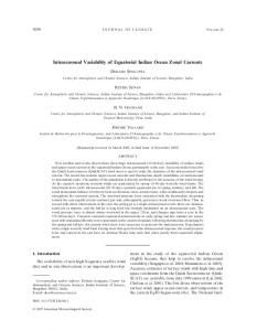
58S was chosen as this is the latitude of maximum SST variability produced by these MJOs. Figure 3 shows the composite longitude–time behavior of the observed and modeled SST anomalies along with the net surface heat fluxes. As weekly SST data (Reynolds and Smith 1994) are used to construct the observed composite (Shinoda et al. 1998), weekly means of the model output are formed prior to compositing. The linear trend along the phase axis at each longitude is eliminated in both the observed and model SST. The slight difference in heat fluxes in these figures results from the use of the 1D model SST to calculate the heat flux used for the 1D model. In general, the amplitude of the model SST variation agrees well with the observed composite, with maximum amplitude occurring in the Indonesian region. As with the observed behavior, the model SST exhibits continuous eastward propagation. However, there are some differences between observation and model. In the western Pacific, during the cooling phase of intraseasonal oscillation, the model SST is cooler than observed (ø0.18C). During the warming phase, a local maximum near 1558E (near phase 22508) occurs in the model SST but is not seen in the observations. In the Indian Ocean, the model SST is noisier than observed, while near 858E, the amplitude of the model intraseasonal SST variation is larger than observed. The minimum model temperature there during the cooling phase (near phase 22008) is cooler by ø0.18C. These differences could be caused by errors in the surface heat flux, by neglected horizontal advection, or by other deficiencies of the 1D model. The weekly SST analyses may also be in error, as problems during other periods have been detected (e.g., Shinoda et al. 1998). Near Indonesia (1258–1358E), there are significant differences. For instance, the amplitude of the intraseasonal SST variation of the model is much larger than observed near 1358E. The 1D model in this region may not be as useful as for other areas. This is a region of shallow oceans interrupted by numerous islands. Response of shelf waters to wind forcing is different from the open ocean. Also, the flux parameterizations derived from open ocean data may not be appropriate near mountainous islands. Furthermore, this region is the center of tidal mixing, which is not included in the 1D model, and it may systematically affect the intraseasonal SST variation (Ffield and Gordon 1996). A 3D model with high resolution is necessary to fully discuss the physical processes that control the intraseasonal SST variation in this region. The SST anomaly, in both model and observations (Fig. 3), propagates eastward along with the net surface heat flux but at approximately a 1/4 cycle lag (10–15 days). If the mixed layer depth is constant, this phase lag should be exactly 1/4 cycle. Thus this suggests that to first order the SST anomalies are driven directly by the surface heat flux variations without regard to vari-
OCTOBER 1998
SHINODA AND HENDON
2675
FIG. 3. Composite SST (8C) anomaly (line contour) from (a) the mixed layer model and (b) the data (Reynolds and Smith 1994) averaged over 2.58–7.58S. Shading indicates net surface heat flux (W m22 ) anomaly calculated from (a) the model SST and (b) the observed SST (Reynolds and Smith 1994). The vertical axis indicates the phase of intraseasonal oscillations obtained from the EOF analysis of OLR data. The linear trend along the phase axis is removed.
ations in mixed layer depth. Mixed layer depth variations can affect the sensitivity of the mixed layer temperature change to the surface heat flux variations and the amount of shortwave radiation that penetrates through the mixed layer. Mixed layer deepening is also indicative of entrainment and, hence, possibly an additional heat flux. While Fig. 3 indicates mixed layer
depth variations may not be important for determining the gross characteristics of the intraseasonal SST, it will be detailed below that both the longitudinal variation in the mean mixed layer depth and the temporal variation of the mixed layer depth over the life cycle of the MJO do exert a pronounced impact on the intraseasonal thermodynamics of the mixed layer.
2676
JOURNAL OF CLIMATE
VOLUME 11
FIG. 4. Average amplitude of composite heat flux (dashed curve), SST (thick curve), and mixed layer depth (dotted curve) at each longitude.
That the mean mixed layer depth impacts the intraseasonal variation of SST can be seen by considering the longitudinal variation of the amplitude of the intraseasonal heat flux (defined here as the maximum minus the minimum of the composite heat flux divided by 2) and of the predicted amplitude of the SST (Fig. 4). The maximum amplitude of the SST occurs near the Indonesian region while the maximum amplitude of the heat flux occurs near the date line. This discrepancy results partly because the mean mixed layer depth (formed by averaging the composite over all phase bins) increases to the east as well (Fig. 4). However, there are discrepancies between the surface heat flux variation divided by the mean mixed layer depth (which gives an estimate of the resulting SST amplitude) and the predicted amplitude of SST. This is possibly because of the large temporal variation of the mixed layer depth over the course of the MJO in the western Pacific, which may significantly affect the amplitude of SST. The question is also raised as to why the mean mixed layer depth increases to the east. Anderson et al. (1996) demonstrated that the mean mixed layer depth produced by the PWP model scales with the equilibrium mixed layer depth, as given by the Monin–Obukov length scale (Niiler and Kraus 1977) Lb 5 u* 3 /B 0 , for a wide range of surface forcings. Here, u* is the surface friction velocity and B 0 is the net surface buoyancy forcing. Note
that the Monin–Obukov scaling is useful only for a positive buoyancy flux and when the subsurface stratification does not play a role in the mixed layer evolution. The equilibrium mixed layer depth, based on the composite mean surface friction velocity and surface buoyancy flux, is shown in Fig. 5a along with the composite mean mixed layer depth from the model integrations. The mean model mixed layer depth is seen to scale reasonably well with the Monin–Obukov length scale except near 1458E. The longitudinal variation of the mean mixed layer depth is also seen to be essentially determined by the longitudinal variation of the surface stress (Fig. 5b), with the mean mixed layer depth increasing to the east in conjunction with the mean surface stress. The mean mixed layer depth near 1458E is much shallower than the Monin–Obukov length. In this region, deepening of the mixed layer is possibly limited by strong stratification beginning near 30–40 m, which is not accounted for in the Monin–Obukov estimate. Also, 1D physics may not be valid in this region as mentioned earlier in this section. The mixed layer depth is also seen to vary intraseasonally over the life cycle of the MJO (Fig. 6). The amplitude of the intraseasonal variation in mixed layer depth increases to the east, consistent with the increase of the amplitude of the intraseasonal variation in net surface heat flux and surface stress (Fig. 4). The impact
OCTOBER 1998
SHINODA AND HENDON
2677
FIG. 6. Composite mixed layer depth (m) averaged over 2.58– 7.58S. Vertical axis is same as in Fig. 3.
mean. This effect is shown in Fig. 7b, where the penetrative radiation is computed both based on the daily mean (but intraseasonally varying) mixed layer depth and based on the composite mean mixed layer depth. In the case of the composite mean (i.e., constant) mixed
FIG. 5. (a) Average Monin–Obukov length (thick curve) and mixed layer depth (dashed curve) at each longitude calculated from the composite. (b) Average wind stress (dashed curve) and surface buoyancy flux (thick curve) at each longitude.
of this intraseasonal variation of mixed layer depth on the response of the mixed layer temperature can be estimated by Q/(rch), where Q is the net surface heat flux minus the shortwave radiation that penetrates through the mixed layer, h is the predicted intraseasonally varying mixed layer depth, c is the specific heat, and r is the density of seawater. Here, Q/(rch) is shown at 1658E (Fig. 7a), which is where the intraseasonal mixed layer depth variation is relatively large. Also shown in Fig. 7a is the Q/(rch) using the composite mean (i.e., constant) mixed layer depth instead of the intraseasonally varying depth. In general, use of the mean depth results in an overprediction of the cooling episode because the intraseasonally varying mixed layer is deeper than the mean at these times (due reduced buoyancy forcing and enhanced surface stress). Using the mean depth also results in an underprediction of the warming episodes because the intraseasonally varying mixed layer is shallower than the mean at these times. The underestimation of the warming using the mean depth is somewhat mitigated by the increase in the penetration of shortwave radiation through the base of the mixed layer when the mixed layer is shallower than the
FIG. 7. (a) Mixed layer temperature tendency estimated from Q/ (rch) for the grid box centered at 58S, 1658E. Here, Q is the surface heat flux, c is the specific heat, and h is the mixed layer depth. The thick line indicates the values calculated from the variable mixed layer depth. The dashed line indicates the values calculated from the mean (i.e., constant) mixed layer depth. (b) Penetrative component of shortwave radiation below the mixed layer. The thick line indicates the values calculated from variable mixed layer depth. The dashed line indicates the values calculated from the constant mean mixed layer depth.
2678
JOURNAL OF CLIMATE
VOLUME 11
FIG. 8. Composite surface heat flux (contour 20 W m22 ) and entrainment heat flux (shading) averaged over 2.58–7.58S. The vertical axis is same as in Fig. 3.
layer depth, the intraseasonal variation of the penetrative shortwave flux results solely from the intraseasonal variation of surface insolation, with increased penetrative flux coinciding with enhanced insolation during the calm–clear phases of the MJO (near 22508 and 11008). Including the intraseasonal variation of the mixed layer depth results in an extra 20 W m22 of penetrative radiation during the calm–clear phases and a 10 W m22 decrease during the windy–cloudy phase, when the intraseasonally varying mixed layer is deeper than the mean. Hence, the intraseasonal variation of penetrative radiation that results from the intraseasonal variation of mixed layer depth tends to counteract the enhanced sensitivity of the mixed layer temperature during the warming phase (when the mixed layer is shallower than mean and less insolation is absorbed in the mixed layer). On the other hand, the reduced sensitivity during the cooling phase, when the mixed layer is deeper than the mean, is compounded because more insolation is absorbed in the mixed layer. Finally, the potential impact of any intraseasonal variation of entrainment heat flux on the mixed layer temperature is examined. The entrainment heat flux is calculated by the following formula: Qent 5 2Q0 2
E
0
2h
Q(z) dz 1 r0 c p
]T , ]t
(2)
where Qent is the entrainment heat flux at the base of the mixed layer, Q 0 is the surface heat flux, Q(z) is the absorption of heat due to the penetrative component of solar radiation, h is the mixed layer depth, T is the mixed layer temperature, cp is specific heat, and r 0 is water density. Figure 8 displays the composite entrainment heat flux, based on hourly model data, as a function of longitude and phase bin. Also shown is the net surface heat flux. The entrainment heat flux is seen to be out of phase with the net surface heat flux, such that when the surface heat flux is most negative, entrainment cooling is a minimum and even acts to warm the mixed layer near 1658E. When the surface heat flux is most positive (during the calm–clear phase of the MJO), the entrainment cooling is a maximum. The large entrainment cooling during
FIG. 9. The vertical temperature profile predicted for 26 November 1992. The profiles are shown at 0300, 0900, 1500, and 2100 LST.
the warming phase, when the intraseasonal mixed layer is shoaling, results from the strong diurnal cycle of insolation coupled with weak winds at this time. Then the mixed layer is extremely shallow during the afternoon and deepens significantly at night, entraining colder water into the mixed layer. An example of such behavior is shown at 1658E during the warming phase of the intraseasonal event in November 1992 (Fig. 9). The afternoon mixed layer shoals to about 1 m and is about 18C warmer than the sub–mixed layer water. Nighttime convection extends to about 8 m deep and thus acts to spread the heat absorbed in the shallow afternoon mixed layer to a significantly deeper layer. During the intraseasonal cooling periods, when the mixed layer is deepening and the diurnal cycle of radiation is weaker due to reduced insolation, diurnally generated entrainment cooling weakens and even entrainment warming results (Fig. 8). The negative surface heat flux at this time cools the mixed layer more than the sub–mixed layer water. Because of the freshness of the mixed layer, a slight, but statically stable, temperature inversion develops. Hence, as intraseasonal deepening of the mixed layer occurs due to reduced buoyancy forcing and increased wind stress, entrainment of warmer sub–mixed layer water occurs. A typical evolution of the mixed layer at 1658E over the course of one particular MJO is shown in Fig. 10. The slight inversion between about 10 and 40 m on day 48, which is when the mixed layer is the warmest, results primarily from absorption of penetrative radiation through the mixed layer in the presence of a salinity stratified mixed layer. As the mixed layer cools and deepens during the cloudy–windy phase of the MJO, the sub–mixed layer does not cool as fast yet remains statically stable due
OCTOBER 1998
2679
SHINODA AND HENDON TABLE 1. Model experiments. Expt 1 2 3 4 5
FIG. 10. Daily average temperature profile predicted on 26 November and 8, 28, and 30 December 1992. Crosses indicate the daily mean mixed layer depth on each day.
to the fresher waters above. Hence, entrainment warming results. This process of entrainment warming is demonstrated by other one-dimensional modeling studies in the warm pool (e.g., Shinoda and Lukas 1995). It is not clear, though, how realistic this is. Inspection of temperature profiles observed at the IMET mooring suggest that inversions below the mixed layer are sometimes observed during COARE (see also Feng et al. 1998). However, it is not as frequent as in the 1D model. Further observational and modeling studies are necessary to pursue this problem. 4. Relative importance of surface fluxes A number of model experiments are conducted to better understand the physical processes that control the intraseasonal SST variation associated with the MJO. These experiments are listed in Table 1. To examine the relative importance of the dominant components of the surface heat, model runs with constant shortwave radiation (expt 1) and constant latent heat flux (expt 2) are performed. To gain insight into the relative importance of buoyancy forcing versus wind-generated turbulence for driving mixed layer variations, the wind stress is held constant in expt 3. To explore the role of freshwater flux for stabilizing the mixed layer, expt 4 is conducted with constant evaporation minus precipitation. Finally, to explore the role of systematic intraseasonal variations of high-frequency (i.e., periods shorter than 40–50 days but excluding the diurnal cycle) forcing for causing intraseasonal mixed layer variations, expt 5 is conducted by compositing the surface forcing prior to running the model. The motivation for this run stems from observations by Hendon and Liebmann
Type Shortwave radiation constant Latent heat flux constant Wind stress constant Evaporation–precipitation constant Composite surface forcing
(1994), which suggest that subintraseasonal convective variability is enhanced during the active convective phase of the MJO. Presumably, such a convective enhancement is also associated with enhanced higher-frequency surface winds, which may produce more mixing and deepening than would be anticipated just from the intraseasonal variation of the surface forcings. The constant values of the surface fluxes used in these experiments are the composite mean fluxes from the original integrations (hereafter referred to as the control integrations). In expt 3, the magnitude of wind stress is kept constant, but the direction is allowed to vary as observed. This was done becasue changes of the wind direction could affect the SST since it can generate inertial oscillations that cause mixing due to the shear at the bottom of the mixed layer. In expt 1, constant daily mean shortwave radiation is prescribed, but a diurnal cycle is retained. In expt 5, the composited surface fluxes are taken from the composite of the control runs. Figure 11 shows the results of expts 1–3 along with the control run for the grid boxes centered at 58S, 1658E and 58S, 958E, which are representative of open ocean conditions in the western Pacific and the Indian Oceans, respectively. In the western Pacific, the amplitude of the SST anomaly in expt 1 and expt 2 is approximately half that for the control run (Fig. 11a). This indicates that the variation of shortwave radiation and latent heat flux are equally important for driving the intraseasonal SST variations there. The SST in the western Pacific for expt 1 is also seen to slightly lag that in expt 2, since the shortwave radiation leads the latent heat flux there for the canonical MJO (e.g., Shinoda et al. 1998). The SST in the western Pacific for expt 3 (constant stress) is nearly identical to the control run, which indicates that the wind stress variation is not as important as the latent heat flux and shortwave radiation for driving the intraseasonal SST (and presumably mixed layer) variation. In the Indian Ocean (Fig. 11b), no clear intraseasonal SST variation is evident in expt 1 (constant shortwave flux), while only a slightly reduced intraseasonal variation is evident in expt 2 (constant latent heat flux). This indicates that intraseasonally varying shortwave radiation is the dominant driver of the intraseasonal SST variation in the Indian Ocean. As for the western Pacific, the wind stress variation appears to be much less important than the surface heat flux variation for driving the SST variations in this region (expt 3). However, the intraseasonal variation of the wind stress does affect the mean SST produced by the model.
2680
JOURNAL OF CLIMATE
FIG. 11. (a) Composite SST predicted at (a) 2.58–7.58S, 1608–1708E and (b) 2.58–7.58S, 908–1008E. Linear trends are removed. The thick curve is from the control run, the dashed curve from expt 1, The dashed–dotted curve is from expt 2, and the dotted curve from expt 3 (see text for details).
That is, the mean SST in the control run (29.628C) is higher than in expt 3 (29.468C). This is caused by entrainment associated with wind variations. Because the water below the mixed layer is often warmer than the mixed layer temperature (due to heating by the penetrating component of shortwave radiation in the presence of a salt-stratified shallow mixed layer), frequent entraining episodes, produced by the high-frequency stress variations (which are absent in expt 3), continually tap into this warmer submixed layer water and a warmer mean mixed layer results. The mixed layer depth variations for expts 1, 2, and 3 and for the control are shown in Fig. 12 for the western Pacific. The largest differences in all these experiments occur during the calm–clear phases of the MJO, when the mixed layer is the most shallow. When any of the surface forcings are held constant, the mixed layer cannot shoal to the full extent achieved in the control run. It appears that the shortwave flux variation is the least important for determining the shallowest depth, presumably because the other two forcings (latent heat and stress) are felt entirely within the mixed layer, no matter how shallow it becomes, while an increasing amount of shortwave radiation penetrates through the shoaling mixed layer. On the other hand, all experiments produce
VOLUME 11
about the same maximum depth during the windy– cloudy phase. Presumably, the mixed layer depth is limited by strong stratification, which even the combined effects of all three forcings cannot overcome. Expt 3 (constant stress) exhibits the largest difference with the control run during the calm–clear phase. However, the difference in SST is not as much as this mixed layer depth difference since a larger portion of shortwave radiation penetrates through the mixed layer in the control run (cf. discussion of Fig. 7 in section 3). Experiment 4 is conducted to examine the impact of enhanced precipitation that occurs before the strongest wind and most negative heat flux during the life cycle of the MJO (e.g., Shinoda et al. 1998). Weller and Anderson (1996) and Anderson et al. (1996) have suggested that the phasing of the precipitation relative to the heat flux and surface stress could have a profound impact on the subsequent evolution of the mixed layer. The evolution of SST in expt 4, however, is quite similar to that of the control (Fig. 13). In fact, the SST difference between the two experiments is less than 0.0358C, which is insignificant compared to the intraseasonal amplitude of 0.258C. Thus, enhanced precipitation before the strong wind and most negative heat flux does not appear to significantly affect the intraseasonal mixed layer variation. The impact of the intraseasonal variation of short timescale surface forcing is explored in expt 5 (Fig. 14). The amplitude of the intraseasonal oscillation in SST in expt 5 is very similar to the control, which suggests that the intraseasonal variation of short timescale surface flux variations does not systematically affect the intraseasonal mixed layer behavior produced by the MJO. 5. Impact of diurnal cycle A strong diurnal cycle of SST is observed during TOGA COARE (Weller and Anderson 1996) during the intraseasonal warming episodes and is largely absent during the intraseasonal cooling episodes. Such behavior is evident in the composite model runs (Fig. 15), where enhanced diurnal SST amplitude coincides with positive surface heat flux and reduced surface stress. Model experiments are conducted to examine the impact of this intraseasonal variation of diurnal cycle on the intraseasonal SST variation. First, the model was forced with the daily mean surface fluxes, calculated from the control run. Thus the mean of daily averaged fluxes is the same as the control run that includes the diurnal cycle. Figure 16 shows the composite SST using these daily mean fluxes along with the composite SST from the control run (hourly fluxes) in the western Pacific, where the intraseasonal variation of diurnal amplitude is largest. Note that no trend is removed in both experiments. During the calm–clear phase of the MJO, when the diurnal cycle of SST is large, the SST computed with daily mean forcing is lower by 0.18–0.188C than the control SST. This dif-
OCTOBER 1998
SHINODA AND HENDON
2681
FIG. 12. Composite mixed layer depth of 10 intraseasonal events at 2.58–7.58S, 1608–1708E for the control run, expts 1, 2, and 3.
ference is significant in comparison to the amplitude of the intraseasonal SST variation (0.38C). This indicates that the diurnal variation of shortwave radiation significantly affects the amplitude and phase of the intraseasonal SST variation. The model was also integrated with the hourly and daily mean surface fluxes from the IMET mooring for the TOGA COARE period. The SST of these experiments is shown in Fig. 17. A similar SST difference between the case of daily mean forcing and hourly forcing is evident, but now the magnitude of the difference
is about 0.28–0.58C. Note that a similar difference is also evident when the model is run using the simple sine model (see section 2) of shortwave radiation (not shown). The SST difference between the experiments with the hourly and daily mean surface fluxes is caused by the difference of the daily mean vertical distribution of heating in the two cases. In the case of hourly forcing, the mixed layer is shallow during the daytime warming period (cf. Fig. 9). Thus, large heating is trapped near the surface and the SST rapidly increases. On the other
FIG. 13. (a) Composite SST at 2.58–7.58S, 1608–1708E. The thick curve is from the the control run and the dashed curve is from expt 4.
FIG. 14. Composite SST anomaly at 2.58–7.58S, 1608–1708E from the control and expt 5. The anomalies were formed by removing the composite mean and linear trend.
2682
JOURNAL OF CLIMATE
VOLUME 11
FIG. 15. Composite amplitude of diurnal SST variation (8C) from the control run along 2.58–7.58S. The amplitude is defined by the daily maximum SST minus daily minimum SST divided by 2. The vertical axis is same as in Fig. 3.
hand, during the nighttime cooling, the mixed layer deepens, and the cooling is distributed over a deeper layer. As a result, the daily mean heating near the surface for the hourly flux case is larger than for the daily mean flux case. Hence, the SST is warmer and the sub–mixed layer is cooler in the experiment with hourly forcing, since a large amount of the daily mean heating is trapped near the surface.
FIG. 17. Predicted SST at 18459S, 1568E for 22 October 1992–2 March 1993 using hourly surface fluxes from the IMET mooring data (thick curve) and daily mean fluxes (dashed curve). (b) The SST difference between the two experiments shown in (a).
6. Conclusions
FIG. 16. (a) Composite SST from the model forced with hourly surface fluxes (thick curve) and daily mean surface fluxes (dashed curve). (b) The SST difference between the two experiments shown in (a).
The atmospheric Madden–Julian oscillation (MJO) produces SST anomalies across the equatorial Indian and western Pacific Oceans with typical amplitude of 0.258–0.38C. Especially large events, such as those which passed over the IMET mooring during TOGA COARE (e.g., Weller and Anderson 1996), produce swings in the warm pool SST of more than 18C. An important aspect of these intraseasonal SST variations is that they exhibit spatial coherence over ø8000 km zonally and ø1500 km meridionally, while propagating eastward along with the atmospheric disturbance associated with the MJO. The entire equatorial Indian Ocean cools and the western Pacific warms when the convective disturbance of the MJO is over the Indian Ocean (e.g., Hendon and Glick 1997; Shinoda et al. 1998). One-half cycle later (about 25 days), when the convective disturbance has shifted eastward to the western Pacific, the equatorial Indian Ocean cools while the western Pacific warms. That these intraseasonal SST anomalies possess such a large spatial scale suggests that they may have potentially large impacts on the global circulation. The role that one-dimensional processes play in forcing these intraseasonal SST anomalies was investigated
OCTOBER 1998
SHINODA AND HENDON
by driving a 1D mixed layer model with observed surface flux anomalies. These surface flux anomalies were developed by Shinoda et al. (1998) based on 10 welldefined MJO events from the period 1986–93. The mixed layer model was integrated for each of the 10 MJO events along 58S from the western Indian Ocean to the date line, which is where the MJO-induced SST anomalies are largest (e.g., Hendon and Glick 1997). A 10-event composite of the model results was formed as described in Shinoda et al. (1998). The simulated composite SST agrees well with the observed composite from the weekly SST analyses, suggesting that 1D processes indeed control the intraseasonal SST behavior across the equatorial Indian and western Pacific Oceans. Recent analyses of the data in the COARE area indicate that the horizontal advection of heat plays an important role in determining the SST variation near the equator during strong westerly wind events (Feng at al. 1998; Ralph et al. 1997; Huyer et al. 1997). Significant cooling was produced by the Yoshida jet and associated strong meridional current acting on the anomalous SST gradient during the cloudy–windy phase of the MJO event during late December 1992. The results of the 1D model forced with fluxes estimated from the IMET mooring, which underestimate the peak cooling during late December, are consistent with the above analyses. However, it is likely that the horizontal advection farther off the equator is not as important as near the equator since there locally forced currents are not as strong as the Yoshida jet on the equator. Also, the present study emphasized the large-scale SST anomalies produced by the MJO, which span more than 108 latitude and typically peak at 58S, coincident with the peak surface heat flux anomalies produced by the MJO. For this scale, the occasional short timescale advection caused by strong wind events may not be important. Further study that uses current and temperature data spanning a larger meridional and zonal extent are required to fully examine the role of horizontal advection in the intraseasonal heat budget of the warm pool. Results from the present 1D study indicate that the MJO produces intraseasonal SST anomalies across the warm pool predominantly via anomalies of shortwave radiation and latent heat flux. Because enhanced latent heat flux only slightly lags enhanced convection and, hence, reduced insolation for the canonical MJO (e.g., Shinoda et al. 1998), these two fluxes act together to perturb the warm pool SST. The relative contribution of the surface insolation anomalies was shown to be greater across the Indian Ocean, where the latent heat flux anomalies are relatively weaker (see also Hendon and Glick 1997) than over the western Pacific. While the intraseasonal evolution of SST is, to first order, governed by the evolution of the surface heat flux anomalies, variations of mixed layer depth were also shown to have an important impact. The mean mixed layer depth across the equatorial Indian and western Pacific Oceans increases toward the east, which thus
2683
means that the sensitivity of the mixed layer temperature to surface heat flux variations decreases toward the east. The mean mixed layer deepens toward the east primarily because the mean surface stress increases toward the east while the net surface buoyancy forcing is more zonally constant. Intraseasonal variations of mixed layer depth were also shown to impact the thermodynamics of the mixed layer. The mixed layer is deepest during the windy– cloudy phase of the MJO and shallowest during the calm–clear phase, when the surface heat flux into the ocean is the greatest. This phasing of mixed layer depth variation relative to the surface heat flux variation results in enhanced sensitivity of the mixed layer temperature change to surface heat flux forcing during the warming phases and reduced sensitivity during the cooling phases of the MJO. However, the enhanced sensitivity during the warming phases was found to be partially offset by an increasing amount of shortwave radiation that penetrates through the base of the shoaling mixed layer. Entrainment cooling during the cloudy–windy phase of the MJO, when the mixed layer is deepening intraseasonally, was found not to enhance the cooling driven by the negative surface heat flux. In fact, entrainment warming often results during this phase. Reduced entrainment cooling and sometimes warming results because of a statically stable temperature inversion that develops at the base of the fresh mixed layer. At the peak warming phase, when the mixed layer is at its shallowest, this inversion develops because of absorption of shortwave radiation that penetrates through the shallow, but fresh, mixed layer. As the mixed layer first starts to deepen during the cloudy–windy phase of the MJO, this warmer water is entrained into the mixed layer. As the mixed layer continues to cool via negative surface heat flux forcing, its freshness allows it to cool slightly more than the sub–mixed layer yet remain statically stable. As the mixed layer then deepens due to increased wind stirring and reduced buoyancy forcing, entrainment of relatively warmer, submixed layer water occurs. However, cold subthermocline water was never entrained into the mixed layer in any of the model runs, suggesting that the intraseasonal surface forcing produced by the MJO is not sufficiently strong to overcome the mean stable stratification present in the warm pool thermocline. However, it is possible that entrainment heat flux is underestimated due to the use of smooth (climatological) initial conditions (see, e.g., Feng et al. 1998). Further study using mooring data is required to examine this problem. The impact of the intraseasonal variation of largescale precipitation associated with the MJO was investigated by running the model with constant evaporation minus precipitation. The freshwater flux associated with the precipitation acts to freshen and stabilize the mixed layer and may lead to a shallower and more sensitive mixed layer. However, the impact on the intraseasonal
2684
JOURNAL OF CLIMATE
SST variation produced by the MJO was shown to be minimal. The reason is postulated to be because the bulk of the precipitation associated with the MJO occurs in conjunction with the windiest conditions and most negative surface heat flux. A shallow, salinity stratified mixed layer thus cannot form at this time (e.g., Weller and Anderson 1996). For the precipitation to have a large impact on the mixed layer thermodynamics would require the bulk of it to fall after the windiest conditions, which would allow a shallow mixed layer to immediately reform. This shallow, fresh mixed layer would then be much more sensitive to the subsequent increased positive surface heat flux during the sunny–calm phase. Anderson et al. (1996) have shown precipitation to play an important role for a specific short timescale warming phase observed at the IMET mooring, whereby sporadic precipitation during the calm phase of the MJO helped lead to the observed rapid recovery of the SST after a pronounced cloudy–windy episode. Our results suggest that this particular precipitation episode observed at the IMET site exhibits little spatial coherence and appears not to be fundamental to the large-scale evolution of the warm pool mixed layer associated with the canonical MJO. Finally, we found that inclusion of the diurnal cycle of shortwave radiation leads both to a warmer mean mixed layer and to larger intraseasonal SST variations associated with the MJO due to the nonlinearity of the system. Inclusion of the diurnal cycle of insolation produces a shallower, warmer mixed layer overlying a colder sub–mixed layer, as compared to that produced by daily mean insolation. Diurnally enhanced mixed layer warming is relatively larger during the calm–sunny phase of the MJO than during the cloudy–windy phase, when the diurnal cycle is almost absent. For the canonical MJO, inclusion of the diurnal cycle of insolation increases the mean SST by about 0.158C and the intraseasonal SST variation by about 20%. Future modeling studies of the maintenance and intraseasonal variation of the warm pool should thus include the diurnal cycle of shortwave radiation. Acknowledgments. We wish to thank Robert Weller for kindly providing the WHOI IMET mooring data. The SRB data were obtained from the NASA/Langley Research Center EOSDIS Distributed Active Archive Center. Insightful comments from the two anonymous reviewers are gratefully acknowledged. This work was supported by a TOGA COARE grant from NOAA’s Office of Global Programs. REFERENCES Anderson, S. P., R. A. Weller, and R. Lukas, 1996: Surface buoyancy forcing and the mixed layer in the western Pacific warm pool: Observation and one-dimensional model results. J. Climate, 9, 3056–3085. Berliand, M. E., and T. G. Berliand, 1952: Determining the net long-
VOLUME 11
wave radiation of the earth with consideration of the effect of cloudiness (in Russian). Izv. Akad. Nauk. SSSR Ser. Geofiz., 1. Cronin, M. F., and M. J. McPhaden, 1997: The upper ocean heat balance in the western equatorial Pacific warm pool during September–December 1992. J. Geophys. Res., 102, 8533–8553. Fairall, C., E. F. Bradley, D. P. Rogers, J. B. Edson, and G. S. Young, 1996: The TOGA COARE bulk flux algorithm. J. Geophys. Res., 101, 3747–3764. Feng, M., P. Hacker, and R. Lukas, 1998: Upper ocean heat and salt balances in response to a westerly wind burst in the western equatorial Pacific during TOGA COARE. J. Geophys. Res., 103, 10 298–10 311. Ffield, A., and A. L. Gordon, 1996: Tidal mixing signatures in the Indonesian Seas. J. Phys. Oceanogr., 26, 1924–1937. Hendon, H. H., and B. Leibmann, 1994: Organization of convection within Madden–Julian oscillation. J. Geophys. Res., 99, 8073– 8083. , and J. Glick, 1997: Intraseasonal air–sea interaction in the tropical Indian and Pacific Oceans. J. Climate, 10, 647–661. Huyer, A., P. M. Kosro, R. Lukas, and P. Hacker, 1997: Upper ocean thermohaline fields near 28S, 1568E, during the Tropical OceanGlobal Atmosphere Response Experiment, November 1992 to February 1993. J. Geophys. Res., 102, 12 749–12 784. Large, W. G., J. C. McWilliams, and S. C. Doney, 1994: Oceanic vertical mixing: Review and a model with a nonlocal boundary layer parameterization. Rev. Geophys., 32, 363–403. Lau, K.-M., and C.-H. Sui, 1997: Mechanisms of short-term sea surface temperature regulation: Observations from TOGA COARE. J. Climate, 10, 465–472. Levitus, S., and T. P. Boyer, 1994: World Ocean Atlas, Vol. 4: Temperature. NOAA Atlas NESDIS 3, 117 pp. , R. Burgett, and T. P. Boyer, 1994: World Ocean Atlas, Vol. 3: Salinity. NOAA Atlas NESDIS 3, 97 pp. Lukas, R., and E. Lindstrom, 1991: The mixed layer of the western equatorial Pacific ocean. J. Geophys. Res., 96 (Suppl.), 3343– 3357. Madden, R. A., and P. R. Julian, 1972: Description of global-scale circulation cells in the tropics with a 40–50 day period. J. Atmos. Sci., 29, 1109–1123. Niiler, P. P., and E. B. Kraus, 1977: One-dimensional models of the upper ocean. Modeling and Prediction of the Upper Layers of the Ocean, E. B. Kraus, Ed., Pergamon, 143–172. Paulson, C. A., and J. J. Simpson, 1977: Irradience measurements in the upper ocean. J. Phys. Oceanogr., 7, 952–956. Price, J. F., C. N. K. Mooers, and J. C. Van Leer, 1978: Observation and simulation of storm-driven mixed layer deepening. J. Phys. Oceanogr., 8, 582–599. , R. A. Weller, and R. Pinkel, 1986: Diurnal cycling: Observations and models of the upper ocean response to diurnal heating, cooling, and wind mixing. J. Geophys. Res., 91 (C7), 8411– 8427. Ralph, E. A., K. Bi, and P. P. Niiler, 1997: A Lagrangian description of the western equatorial Pacific response to the wind burst of December 1992. J. Climate, 10, 1706–1721. Reynolds, R. W., and T. M. Smith, 1994: Improved global sea surface temperature analyses using optimum interpolation. J. Climate, 7, 929–948. Shinoda, T., and R. Lukas, 1995: Lagrangian mixed layer modeling of the western equatorial Pacific. J. Geophys. Res., 100, 2523– 2541. , H. H. Hendon, and J. Glick, 1998: Intraseasonal variability of surface fluxes and sea surface temperature in the tropical western Pacific and Indian Oceans. J. Climate, 11, 1685–1702. Spencer, R. W., 1993: Global oceanic precipitation from the MSU during 1979–91 and comparisons to other climatologies. J. Climate, 6, 1301–1326. Waliser, D. E., and N. E. Graham, 1993: Convective cloud systems and warm-pool sea surface temperatures: Coupled interactions and self-regulation. J. Geophys. Res., 98 (D7), 12 881–12 893. Webster, P. J., and R. Lukas, 1992: TOGA COARE: The Coupled
OCTOBER 1998
SHINODA AND HENDON
Ocean–Atmosphere Response Experiment. Bull. Amer. Meteor. Soc., 73, 1377–1416. Weller, R. A., and S. P. Anderson, 1996: Surface meteorology and air–sea fluxes in the western equatorial Pacific warm pool during the TOGA Coupled Ocean–Atmosphere Response Experiment. J. Climate, 9, 1959–1990. Whitlock, C. H., and Coauthors, 1995: First global WCRP shortwave surface radiation budget dataset. Bull. Amer. Meteor. Soc., 76, 905–922.
2685
Yoshida, K., 1959: A theory of the Cromwell current and of the equatorial upwelling—An interpretation in a similarity to a coastal circulation. J. Oceanogr. Soc. Japan, 15, 159–170. Zhang, C., 1996: Atmospheric intraseasonal variability at the surface in the tropical western Pacific Ocean. J. Atmos. Sci., 53, 739– 758. Zhang, Q., 1995: The oceanic response to atmospheric forcing in the western equatorial Pacific. Ph.D. thesis, University of Rhode Island, 164 pp.