Mixed Model Assembly Line Balancing Problem under Uncertainty S.M.J Mirzapour AI-e-hashem 1, M.B Aryanezhad 2, H. Malekly 3, S.J. Sadjadi 4
3
1,2,4 Department of Industrial Engineering, University of Science and Technology, Tehran, Iran Department of Industrial Engineering, Graduate School, Islamic Azad University-South Tehran Branch, Member of Young Researchers Club, Tehran, Iran (1
[email protected], 2
[email protected], 3
[email protected])
ABSTRACT A common assumption in the literature on mixed model assembly line balancing problem is that the task duration is known and deterministic but may differ among various models. In this paper, we present a robust optimization formulation for dealing with task duration uncertainty in a mixed model assembly line balancing problem (RMALB-P) in which task duration can vary in a specific range. RMALB-P is aim to minimize the sum of costs of the stations and the task duplication. Task duplication means that a task which is common to multiple tasks can be assigned to different stations for different models. Finally, RMALB-P is solved optimally and implemented in mixed model assembly lines of IRAN KHODRO Company. The results are compared with the previous existing balance to show the effects of the data uncertainties on the performance of assembly line outputs. The results indicate that the robust balancing approach can be a relatively more reliable method for balancing the mixed model assembly lines. Keywords: mixed model, assembly line balancing, robust optimization, mixed integer programming optimization.
1.
INTRODUCTION
1.1. Assembly line balancing Modeling of assembly lines has been an active area of research for about the last four decades. A heavily studied problem is the problem of balancing an assembly line by assigning the operations required by a single model to a number of stations. When there is only one model of a product that is being assembled on the line, the resulting problem is called the simple assembly line balancing problem (SALBP). The solution approaches to this problem have two typical variations. The problem of assigning operations to stations is formulated with the objective of minimizing the number of stations used to meet a target cycle time (SALBP-1), or with the objective of minimizing the cycle time given a predetermined number of stations (SALBP-2). In either case, precedence relations among the required operations constitute a part of the constraints of the problem. Comprehensive surveys of related research appear in [1-3]. The mixed model assembly line is a more complex environment in which several variants of the product, referred to as models, are assembled simultaneously on the line. The line balancing problem in a mixed model environment (MALB-P) involves the assignment of tasks of all models to the workstations. This problem is much more complex since it entails the additional considerations of the interactions among the assembled models. This problem has been investigated during the last four decades, where some of the earliest works were
those of Thomopoulos [4, 5]. For recent surveys of the various types of assembly line balancing problems (see [6, 7] and [26, 27]). Due to the increasing importance of the mixed model assembly lines in modem industry, several works have addressed the MALB-P in the last few years (see [8-14] and [28]). Most of the research on the subject has adopted an approach in which each task that is common to several models is restricted to a single workstation. When such restriction is considered, the balancing procedure becomes similar to the one used for solving the SALB-P, and consists, in general, of balancing a single combined model, which represents the union of all tasks of all the assembled models. In our proposed model, the task assignment constraint is relaxed. Although a task of a particular model must be assigned to a single station, tasks common to different models may be assigned to different stations (task duplication). Some additional costs are associated with task duplication, such as: costs of machinery and tool duplication, costs associated with the increased complexity of line operation (training, learning) and cost of inventory management. 1.2. Robust optimization The classical paradigm in mathematical programming is to develop a model which assumes that the input data is precisely known and equal to some nominal values. This approach, however, does not take into account the influence of data uncertainties on the quality and feasibility of the model. It is therefore conceivable that
978-1-4244-4136-5/09/$25.00 ©2009 IEEE
233
as the data take values different from the nominal ones, several constraints may be violated, and the optimal solution found using the nominal data may no longer be optimal or even feasible. This observation raises the natural question of designing solution approaches that are immune to data uncertainty; that is, they are "robust." To illustrate the importance of robustness in practical applications, we quote from the case study by Ben-Tal and Nemirovski [15] on linear optimization problems from the Net Lib library "In real-world applications ofLinear Programming, one can not ignore the possibility that a small uncertainty in the data can make the usual optimal solution completely meaningless from a practical viewpoint." Naturally, the need arises to develop models that are immune, as far as possible, to data uncertainty. The first step in this direction was taken by Soyster [16], who proposes a linear optimization model to construct a solution which is feasible for all data that belong in a convex set. The resulting model produces solutions that are too conservative in the sense that we give up too much of optimality for the nominal problem in order to ensure robustness ([ 16]). Soyster [16] considers the linear optimization problem
cx
PI: maximize
subject to
~ L...J aijxj -< bii,
i=l, ..., m
(1)
j=l Xj~O,
The uncertainty is assumed to affect the aij. In robust optimization technique, for modeling uncertainty in data, consider a particular row i of equation (1) and let J, represent the set of coefficients in row i that are subject to uncertainty. Each entry aij, j EJi is modeled as a symmetric and bounded random variable which takes values in [aij-aij, aij+aij] centered at the point aij, nominal value, and aij measures the precision of the estimate. Soyster [16] shows that the problem is equivalent to P 2 : maximize
subject to
cx
:ta;jxj~bi,
uncertainty sets. However, a practical drawback of such an approach is that it leads to nonlinear, although convex models, which are more demanding computationally than the earlier linear models by Soyster [16] (see also [15] and [21]). Ben-Tal and Nemirovski [15] proposed the following robust problem P 3 : maximize
subject to
(2)
j=l Xj~O,
where ~j = sup jc Ji (aij) . Soyster [16] admits the highest protection. It is also the most conservative in practice in the sense that the robust solution has an objective function value much worse than the objective function value of the solution of the nominal linear optimization problem. A significant step forward for developing a theory for robust optimization was taken independently by [15] and [17-20]. To address the issue of over conservatism, these papers proposed less conservative models by considering uncertain linear problems with ellipsoidal uncertainties, which involve solving the robust counterparts of the nominal problem in the form of conic quadratic problems [18]. With properly chosen ellipsoids, such a formulation can be used as a reasonable approximation to more complicated
Vi
Laijxj + LClijYij +Oi j
(3)
j e.J,
-Yij~Xj-zij~Yij
Vi,jEJi
x,Y~O,
In model (3), Xj, Yij and zij are decision variables. Under the model of data uncertainty, the probability that the constraint i is violated at most is k = exp (-n2i / 2) where k is the reliability level (e.g. k = 10-6) . Therefore, the reliability level is controlled when n is changing. Bertsimas and Sim [22-24] and Bertsimas et al. [25] proposed another approach for robust linear optimization that retains the advantages of the linear framework of Soyster [16]. More importantly, their approach offers full control on the degree of conservatism for every constraint. They protected against violation of constraint i deterministically, when only a prespecified number T, of the coefficients changes; that is, they guaranteed that the solution is feasible if less than r i uncertain coefficients change. Moreover, they provided a probabilistic guarantee that even if more than ~ change, then the robust solution will be feasible with high probability. They define the scaled deviation from nominal value of aij as aij -~j llij=-"-
(4)
-.
where aij and aij are uncertain data and nominal value, respectively, and aij measures the precision of the estimate. It is clear the 11ij has an unknown but symmetric distribution which takes values in [-1,1]. Although the aggregated scaled deviation for constraint i could take any value between [-n,n], but it is limited to n
i=l, ....m
cx
LlJij j=l
~ r;
(5)
Vi
where T, is not necessarily integer and takes values in the interval [0, IJil]. The role of this parameter is to adjust the robustness of their proposed method against the level of conservatism of the solution. T, is called the budget of uncertainty of constraint i. 1. If Ti = 0, there is no protection against uncertainty. 2. If f i = IJil, the i th constraint of the problem is completely protected against uncertainty. 3. If F, E (0, IJil), the decision-maker makes a trade-off between the protection level of the constraint and the degree of conservatism of the solution [22]. In this approach, the set J, is defined as J, = ((auJ I aij = aij + iiij1]ij V i.], with
Z={'7lhll';I'~'7ij,;r;, Vi},
1] E
Z)
(6) (7)
234
i:aijXj = j=1
:t
(G;j + ai/7ij)X j +
j=1
:t
aij17ijXj'
Vi.
(8)
j=1
Now, problem (PI) can be reformulated as follows Ps: maximize c'x subject to
:t
ax. + min
j=1
:t
aX17 < b
17i EZ i j=1
1J )
1J }
1J -
Vi,
(9)
1
x)~o,
min ~ a.. x .n.. for a given i is equivalent to z L..J lJ r/» )=1
r/iE
i
P 6 : maximize ~"I
LJaij -,
I
'7ij
j=!
subject to
n
~
LJTJij:::;
r
(10)
Vi.
i
j=1
0:::; TJij :::; 1 x)
Vj.
~O,
5. The station time of each model must not exceed the model's cycle time. 6. Each task should be assigned to exactly one station in each model. The input to the model includes the following data: number of models; interval of duration for each task in each model; a set of precedence constraints (the set of precedence constraints may be represented for convenience as a directed a cyclic graph, a precedence diagram, where each node represents a task and each directed represents a precedence relation); cycle time for each model (the inverse of the required production rate of each model); a cost for each station to be opened in the assembly line; and finally, a duplication cost for each task. The solution of the MALB is a configuration of an assembly line in which all tasks of all models are assigned to workstations and the cycle time and precedence constraints for each model are satisfied.
Duality of (10) is expressed as follows ([23])
2.1. Problem formulation
P 7: maximize q.T, + ~ r..
The notation used for the formulation of the problem is as follows n Total Number of different assembly tasks. m number of models to be assembled on the line. tij process time of task i (i = 1, ..., n) when performed on model} (j = 1, ..., m). IPij set of immediate predecessors of task i in model}. Cj required cycle time for model}. Sc station cost; fixed cost associated with each station TCi task cost; fixed cost associated with each station to which task i is assigned. z number of stations to be used in the assembly line Xijk is equal to 1; if task i of model} is assigned to station k and equal to 0; otherwise. Note that since the number of stations is a decision variable, we use the number of tasks, n, as an upper bound on this value. ~ik is equal to 1; if task i of any of the models IS assigned to station k, and equal to 0; otherwise. The original formulation is as follows MALB-P:
11
subject to
~lJ jEJ;
qi + If) ~ aij/x)1 rij
~
Vi,}
E
J i,
(11)
Vj E J i
0
qi ~ 0 Vi, where qi and rij are the dual variables. When (11) is applied to (9), the robust formulation based on Bertsimas and Sim ([22-24]) and Bertsimas et al. [25] is changed as follows P s: maximize c'x
(12) - y) ~
x)
~ y)
V}
x, y, r, q ~ 0,
where y is a decision variable for make the absolute term (Ixjl) to linear one. The robust counterparts they proposed are linear optimization problems, and thus their approach readily generalizes to discrete optimization problems and applied here in this paper for modeling RMALB-P.
3.
MODEL DESCRIPTION
We shall now specify original MALB model which aims to minimize the total cost associated with the design of the assembly line and then is reformulated as a RMALB according to robust optimization model (4). The model assumptions are specified as follows: 1. Multiple similar models of the same product are assembled on the same line. 2. Task duration is uncertain and can vary in a specific range. 3. A cycle time is associated with each model type. 4. The duration of a task is not longer than the cycle time of the associated model (no use of stations in parallel).
minimize {sc.z+
tTCi~~ik}
subject to ~ 1 LJXijk =
\-I.
(13) (14)
•
v i.],
k=l
:tk,xVjk s; :tt.XUj/ Vv,j,u S.t. v E IPuj k=1
(15)
1=1
:t
Vj k,
Xijkiij S; C j
(16)
i=l
z > :tk,Xijk
(17)
Vi,j,
k=1
1 m ;ik~-·Lxijk m
Vi,k,
(18)
j=l
Xijk'~ik E {O,l}
(19)
The objective function (13) minimizes the total cost (the sum of the station and task costs). Constraint set (14)
235
ensures that every task required by each model is assigned to exactly one station. The precedence relationships among tasks are captured by constraints set (15) which ensure that a task will be assigned to a certain station k only if its immediate predecessors have all been assigned to that station or to an upstream station. Constraint set (16) restricts the total process time of each model at each station not to exceed the model's cycle time. Constraint set (17) determines the total number of stations to be used (equal to the greatest station index number of all tasks and models). Constraint set (18) examines whether task i of any model is assigned to station k. Finally, constraint set (19) defines all decision variables as binary. Using robust optimization model (Pg) MALB-P is converted to RMALB-P as follows
RMALB-P: minimize
Sc·z+ ~TCiB~ik 11
{
11
(20)
}
presented in Figure.I. Data concerning tij (deterministic task durations) as well as ~j' u (data uncertainty) and
t
also TCi values (in cost units) are given in Table 1. As we can observe from Figure. 1, the set of tasks performed in Model II is not in the same order as the set of tasks performed in Model I. In addition, the tasks common to both models do not necessarily require the same amount of time to perform.
Modell
FigureI. Precedence diagrams for Models I and II. Table 1. Process times and task costs for the example problem tij
n
=1
(21)
Vi,},
k=l
"fl.x ~ "f/x
Vv,l,u
,lj/
Vj k
k=l
s.t. vE Ip,1j
n
i=l
i=l
qj
(22)
1=1
n
LXijk'~j+qjrj+LlfjSCj
+ Ifj ~ ~jYi'
(23)
V},k,
Vi,}
(24)
Vi,},k,
(25)
- Yi S Xijk S Yi' n
Z
~ Lk,xijk
(26)
Vi,},
k=l
1
m
~ik ~-'LXijk
(27)
't;Ji,k,
m )=1
Xijk'~ik
E
{O,l}
(28)
where qi and rij are the dual variables. tij is modeled as a symmetric and bounded random variable that takes values
in
[I.. I}
t..
I}'
1.. + t.. ] I}
I}
.
Moreover
,
qjrj
+~ ~ Ifj i=1
represents the extra task duration (or shortness thereof) where we want to take into account in controlling the system from a worst-case perspective. As mentioned before, this robust formulation retains linearity and can be solved with mathematical programming solvers readily. 4.
EXPERIMENTAL RESULT
In this section a simple example is presented to illustrate the problem and emphasize the importance of incorporating robust approach. Let Yi be the efficiency of assembly line for model } and Y;
0=
100 x
Model I
Task
subject to LXijk
:t:t /(:t:t tikXijk
1=1 k=1
1=1 k=1
Xijk x
m.F(~)ikXi;k) Consider a i=1
product with two models (m = 2). The assembly process of each model consists of a series of assembly operations selected out of a group of five possible tasks (n = 5). The precedence diagrams for both models are
Model II
tij
1 2
6
6
4
3 4 5
4 2
4 6 4 2
6
Model II {ij
tij
t;j
2 5 4 1 3
2 5 4 1 3
TCj
iii
11 5 8 3 2
The station cost, SC, is equal to 10 cost units and parameter I j is equal to 2 for all i. The required cycle times for Models I and II are 8 and 9 time units respectively. In Table 2, two balancing solutions for th~ example problem are presented. The first solution is an optimal solution with deterministic task duration and the second solution is an optimal solution subject to data uncertainty. The table is divided into blocks each representing a station. In every block, the cells under the "assigned tasks" column specify, for every model, the tasks assigned to that station. The cells under the "cumulative time" column indicate, for every model, cumulative time of each station. The cells under the Yj column indicate, for every model, the percent of efficiency of assembly line. For example 91.6% (efficiency of assembly line for model I under the deterministic assumption) is calculated as: (6+8+8)/ (Jxmax (6, 8, 8)) and 83.3% (efficiency of assembly line for model II under the deterministic assumption) is calculated as (9+6)/ (Zxmax (9, 6)). According to Table 2, although robust formulation (RMAL-P) leads to an assembly line with 4 stations in comparison with MALB-P with 3 stations, RMALB model retains efficiency of assembly line at least the same as the case of MALB model. In fact, since task duration is uncertain, RMALB model, spending more money through opening more stations, tries to keep the assembly line efficiency as close as the case of deterministic condition. In other words, task duration perturbations cannot influence the efficiency of the assembly line when using RMALB model. Note that when, under the deterministic assumption, some perturbation is occurred in real cases, cycle time is the
236
first and the most important thing that is changed. Then cycle time influences the production planning and finally affects the due dates. Thus, in real world, because of the inevitability of perturbation especially in process times, nature of the cycle time which is the basic parameter of the production planning is converted to a variable (instead of a constant parameter). This phenomenon is named
units of various passenger cars and vans. By 2006 IKCO was producing 550,000 vehicles. The opening of the country's largest car assembly plant in Khorassan in July 2008 is expected to increase capacity with the ability to tum out 100,000 vehicles per annum by late 2009. However, it will not necessarily increase production. Because of the wide use of mixed model assembly lines in automotive industry, we applied our
Table 2. Solutions of the example problem Solution type
Objective value
MALB
69
RMALB
76
Model I
II I II
---_._------
r, 91.6 83.3 91.6 83.3
Station 1 Assigned tasks
Cumulative time
1 1,3,5 2
6min 9min 4min
Station 2 Assigned tasks
Cumulative time
2,4 2,4 1 1,5
8min 6min 6min 5min
here as "interior bullwhip effect" which directly influences the production scheduling undesirably, and these undesirable perturbations are not removed and accumulate along the assembly line. Large amount of work in process between the stations and a manifest deviation from the expected due date are two ultimate interior bullwhip effect. Anyway "interior bullwhip effect" can be controlled using a robust assembly line balancing method. On the other hand the readers maybe note that RMALB model leads to increase the objective value in comparison with the case of deterministic condition (Table 2). This excess cost arises from the cost of opening more stations to control the perturbations. We shall now specify using a simple example where such a situation maybe occurred if data uncertainty is ignored while assembly line balancing is done under the deterministic assumption.
Station 3 Assigned tasks
Cumulative time
3,5
8min
3 3
6min 4min
Station 4 Assigned tasks
Cumulative time
4,5 2,4
6min 6min
proposed model in IKCO, and the experimental result is reported in this paper. A wide set of real case problems (IKCO) has been implemented to analyze the influence of the proposed model on the total cost of assembly line and its efficiency, which has been assumed as performance index in the assembly line balancing (Table 3). In all problem cycle time for all models are set to 10 and dimension of problems are shown in Table 3. max' are the average, maximum In Table 3 and minimum efficiency of assembly line among different models, respectively. Note that for the same of simplicity, we only report the average, maximum and minimum efficiency of assembly line in each problem. In order to compare the performance of two proposed models, (MALB against RMALB) maximum efficiency of line for problems PI to P lO are shown schematically
r, r
rmin
Table 3. Result of Problems PI to P lO MALB Dimension Objective Problem (model*part) value PI 2x5 59 P2 3x5 88 4x5 98 P3 5x6 130 P4 5x8 142 Ps P6 s-ro 223 P7 5x 15 258 5x20 384 Ps 10x25 750 Pg 10x30 822 P IO *Note that all data are round up
5.
r,
rmax , rmin
72.0, 73.0, 71.0* 78.0, 88.0, 57.0 86.0, 100.,74.0 81.0, 95.0, 65.0 79.0, 100., 66.0 86.0,95.0, 72.0 80.0, 100., 55.0 77.0, 85.0, 55.0 82.0, 90.0, 75.0 75.0, 78.0, 70.0
CASE STUDY
Iran Khodro (IKCO) is a public joint stock company with the objective of creation and management of factories to manufacture various types of vehicles and parts as well as selling and exporting them. The company has become the largest vehicle manufacturer in the Middle East. In Iran, it is the largest vehicle manufacturing company, having an average share of 65 percent of domestic vehicle production. In 1997, IKCO broke its own production record by producing 111,111
#opened station 3 3 4 5 7
8 12 18 20 25
RMALB Objective Value 69 108 113 175 165 241 284 409 801 853
r
rmax
83.0, 77.0, 87.0, 82.0, 85.0, 88.0, 89.0, 82.0, 91.0, 88.0,
, rmin
92.0, 75.0 80.0, 70.0 100., 67.0 100., 60.0 100.,70 .0 100., 83.0 95.0, 70.0 85.0, 75.0 100.,85.0 94.0, 75.0
#opened station 4 5 5 6 8 10 15 20 23 28
in Figures 2. As we can see in Figures 2, not only RMALB solution is not less efficient against MALB, but also, most of the time RMALB leads us to have a more efficient solution, considerably. As mentioned before these aforementioned benefits of RMALB arise from spending more money through opening more stations. In Figures 3, the objective value and the number of opened stations for MALB solution against RMALB are presented. As shown in Figure 3, the objective value and also number of opened stations in RMALB are greater than the case of MALB in all
237
problems. But this extra station protected the cycle time from violation that could be occurred via perturbations in the manufacturing systems.
p i
p2
p3
p4
p!">
p6
p7
pH
p9
p IG
Figure 2. Maximum efficieny ofline among models for p] to P IO using RMALB against MALB
900 ,--- - - - - - - - - - 800
~ 800 •
>00
o
'00
1- - - - - - - - - -
+ - - - - - - - - -1
1 ,oo t- - - - 100
_
RM A l B
l--::.~=':::;-:==------pi
p2
p .J
p4
p"
p6
p7
p8
pO)
p lO
Figure 3. Objective value of P, to P IO using RMALB against MALB
6.
CONCLUSION
We have proposed a robust optimization formulation for dealing with task duration uncertainty in a mixed model assembly line balancing problem in which task duration can vary in a specific range. First, we have presented an original model under the deterministic assumption and in the next step, using robust optimization ideas, we have developed an equivalent robust model under uncertainty which is a mixed integer programming (the same class as the original model). The most important effect of uncertainty especially in task duration is that the cycle time of assembly line is violated and leads us to have the problem of assembly line balancing remains to be solved. Our approach is a solution for mixed model assembly line balancing problem under the task duration uncertainty and opening more stations which could control the task duration perturbations.
REFERENCES [I] Baybars, I., "A survey of exact algorithm for the simple assembly line balancing problem", Management Science , 32, 909-932, 1986 [2] Ghosh, S., R.J. Gagnon, "A comprehensive literature review and analysis of the design, balancing and scheduling of assembly systems", International Journal of Production Research 27, 637--670, 1989 [3] Scholl, A., C. Becker, "State-of-the-art exact and heuristic solution procedures for simple assembly line balancing", European Journal of Operational Research, 168. 694-715, 2005 [4] Thomopoulos, N.T., "Line balancing-sequencing for mixed-model assembly", Management Science, 14, 59- 75, 1967 [5] Thomopoulos, N.T., "Mixed model line balancing with smoothed station assignments", Management Science 16,
593-603,1970 [6] Erel, E., S.C. Sarin, "A survey of the assembly line balancing procedures", Production Planning & Control, 9 (5), 414-434, 1998 [7] Becker, C., A. Scholl, "A survey on problems and methods in generalized assembly line balancing", European Journal of Operational Research, 168 (3), 666- 693, 2006 [8] Erel, E., H. Gokcen, "Shortest-route formulation of mixed-model assembly line balancing problem", European Journal of Operational Research, 116, 194-204, 1999 [9] Merengo, c., F. Nava, A. Pozzctti, "Balancing and sequencing manual mixed-model assembly lines", International Journal ofProduction Research, 37 (12), 2835-2860, 1999 [10] Matanachai, S., C.A. Yano, "Balancing mixed-model assembly lines to reduce work overload", liE Transactions, 33, 29--42,2001 [11] Vilarinho, P.M., A.S. Simaria, "A two-stage heuristic method for balancing mixed-model assembly lines with parallel workstations", International Journal of Production Research, 40 (6), 1405-1420,2002 [12] Karabati, S., S. Sayin, "Assembly line balancing in a mixed-model sequencing environment with synchronous transfers", European Journal ofOperational Research 149 (2), 417--429,2003 [13] Xhao, X., K. Ohno, B.S. Lau, "A balancing problem for mixed model assembly lines with a paced moving conveyor", Naval Research Logistics 51, 446--464, 2004 [14] Bukchin, Y., I. Rabinowitch, "A branch-and-bound based solution approach for the mixed-model assembly line-balancing problem for minimizing stations and task duplication costs", European Journal of Operational Research, 174,492-508,2006 [15] Ben-Tal, A., A. Nemirovski, " Robust solutions of linear programming problems contaminated with uncertain data", Math. Program, 88 411--424, 2000 [16] Soyster, A. L., "Convex programming with set-inclusive constraints and applications to inexact linear programming", Oper. Res. 21 1154-1157,1973 [17] Ben-Tal, A., A. Nemirovski, "Robust convex optimization", Math. Oper. Res., 23 769-805,1998 [18] Ben-Tal, A., A. Nemirovski., "Robust solutions to uncertain programs",Oper. Res. Letts., 251 -13,1999 [19] El-Ghaoui, L., H. Lebret, "Robust solutions to least-square problems to uncertain data matrices", SIAM J. Matrix Anal. Appl, 18 1035-1064, 1997 [20] El-Ghaoui, L., F. Oustry, I-I. Lebret, "Robust solutions to uncertain semidefinite programs" . SIAM J. Optim., 9 33-52, 1998 [21] Ben-Tal, A., S. Boyd, A. Nemirovski, "Extending scope of robust optimization: Comprehensive robust counterparts of uncertain problems", Math. Program, Ser. B 107, 63- 89, 2006 [22] Bertsimas, D. M., Sim, " Robust discrete optimization and network flows", Math. Program, Vol. 98, No. 1-3,49-71 ,2003 [23] Bertsimas, D., M. Sim, "The price of robustness", Operations Research, 52 (I), 35-53, 2004 [24] Bertsimas, D., M. Sim, "Tractable approximations to robust conic optimization problems", Mathematical Programming, 107 (I), 5-36, 2006 [25] Bertsimas, D., D. Pachamanova, M. Sim, " Robust linear optimization under general norms", Operations Research Letters, 32, 51Q----516, 2004 [26] Boysen N., M. Fliedner, A. Scholl, "A classification of assembly line balancing problems", European Journal of Operational Research, 183,674--693,2007 [27] Boysen N., M. Fliedner, A. Scholl, "Assembly line balancing: Which model to use when'!" Int. J. Production Economics 111, 509-528, 2008 [28] Van Hop N., "A heuristic solution for fuzzy mixed-model line balancing problem", European Journal of Operational Research, 168,798-810,2006
238