Mixed-precision training of deep neural networks using computational memory Nandakumar S. R.,1, 2, a) Manuel Le Gallo,1 Irem Boybat,1, 3 Bipin Rajendran,2 Abu Sebastian,1, b) and Evangelos Eleftheriou1 1) IBM
Research – Zurich, 8803 R¨uschlikon, Switzerland. Jersey Institute of Technology (NJIT), Newark, NJ 07102, USA 3) Ecole Polytechnique Federale de Lausanne (EPFL), 1015 Lausanne, Switzerland 2) New
arXiv:1712.01192v1 [cs.ET] 4 Dec 2017
(Dated: 5 December 2017)
Deep neural networks have revolutionized the field of machine learning by providing unprecedented human-like performance in solving many real-world problems such as image and speech recognition. Training of large DNNs, however, is a computationally intensive task, and this necessitates the development of novel computing architectures targeting this application. A computational memory unit where resistive memory devices are organized in crossbar arrays can be used to locally store the synaptic weights in their conductance states. The expensive multiply accumulate operations can be performed in place using Kirchhoff’s circuit laws in a non-von Neumann manner. However, a key challenge remains the inability to alter the conductance states of the devices in a reliable manner during the weight update process. We propose a mixed-precision architecture that combines a computational memory unit storing the synaptic weights with a digital processing unit and an additional memory unit accumulating weight updates in high precision. The new architecture delivers classification accuracies comparable to those of floating-point implementations without being constrained by challenges associated with the non-ideal weight update characteristics of emerging resistive memories. A two layer neural network in which the computational memory unit is realized using non-linear stochastic models of phase-change memory devices achieves a test accuracy of 97.40% on the MNIST handwritten digit classification problem. I.
INTRODUCTION
Deep neural networks (DNN) including multilayer perceptrons, convolutional neural networks, deep belief networks, and Long-Short-Term-Memories are loosely inspired by biological neural networks in which parallel processing units called neurons are interconnected by plastic synapses. By tuning the weights of the interconnections these networks are able to solve problems which are intractable by conventional algorithms. Through a combination of factors, such as the availability of massive labeled datasets and the highly parallel matrix manipulations offered by modern GPUs, these networks have recently achieved considerable success in numerous applications1 . A DNN comprises multiple layers of neurons interconnected by synapses. Training of DNNs refers to the process of finding appropriate synaptic weights such that after the training process, the network is able to perform various classification tasks with sufficient accuracy. Typically, this is achieved by a supervised training algorithm known as backpropagation. During the training phase, the input data is forwardpropagated through the neuron layers with the synaptic network performing a multiply-accumulate operation. The final layer responses are compared with input data labels and the errors are back-propagated. All the synaptic weights are updated to reduce the error. This forward-backward data propagations and weight updates are repeated several times over the entire training data set. This brute force approach to training neural networks is computationally intense and, in spite of the
a) Electronic b) Electronic
mail:
[email protected] mail:
[email protected]
availability of computing resources such as the GPUs, is very time-consuming. Also, the high power consumption of this training approach makes its application prohibitive in several emerging domains such as internet of things and edge computing. Much of the inefficiency arises from the fact that the DNNs are trained using conventional von Neumann computing systems where the physical separation between the memory and processing units leads to constant shuttling of data back-and-forth between them. Recently, there is a significant interest in designing non-von Neumann co-processors for training DNNs. A system comprising dense crossbar arrays of resistive memory devices has been proposed to perform the various steps involved in the training of DNNs2–4 . The devices, also referred to as memristive devices, store information in their conductance states5,6 and can be used to represent the synaptic weights. The matrixvector multiplications needed during the propagation of data in the network can then be computed as a result of Kirchhoff’s circuit laws. Weight updates can be applied by modifying the conductance levels of the resistive memory devices by applying appropriate electrical pulses. However, this approach can achieve satisfactory training accuracy only with ideal, not-yet-available resistive memory devices3 . The experimental demonstrations based on existing resistive memory devices have achieved reduced classification accuracies owing to the inability to achieve precise conductance changes in the memristive devices2,7 . A related research area that is gaining a lot of traction is in-memory computing or computational memory. Here, physical attributes of the memory devices are exploited to perform computations in a non-von Neumann manner. There are recent demonstrations of performing bulk bit-wise operations8 , matrix-vector multiplications9–12 and finding temporal correlations using such a memory unit13 . One major issue in
2 this field is the limited precision of the individual units of the computational memory. Recently, we proposed the concept of mixed-precision in-memory computing to counter this challenge12 . The essential idea here is to use the low-precision computational memory unit in conjunction with a precise computing unit. The benefits of areal/energy/speed improvements arising from computational memory are retained while addressing the key challenge of inexactness associated with computational memory. As an example, we presented an iterative solver for systems of linear equations. Meanwhile, there are some key developments taking place at the algorithmic front with respect to training DNNs using digital arithmetic with reduced precision14–18 . Recent work shows that it is possible to have binary precision for the weights used in the multiply-accumulate operations (during the forward and backward propagations) as long as the precision of the stored weights in which gradients are accumulated is retained16 . This indicates the possibility of accelerating the DNN training using programmable low precision computational memory, provided we address the challenge of reliably transferring the high precision gradient to them. In this article, we present a mixed-precision architecture based on computational memory to train DNNs. We investigate various undesirable attributes of the constituent devices in such a computational memory unit and show how the proposed architecture is designed to cope with them. Finally, the DNN training performance of the mixed-precision scheme is evaluated where computational memory devices are realized using stochastic models based on 90 nm phase-change memory characterization.
II.
COMPUTATIONAL MEMORY: THE KEY CHALLENGES
Non-volatile resistive memory devices have several attributes making them suitable candidates for building computational memory elements. These devices operate based on a variety of physical mechanisms such as field driven atomic rearrangement (metal-oxide based resistive memory19 (ReRAM) and conductive bridge memory (CBRAM)20 ), spintronic effects (spin transfer torque based magnetic memory (STT-MRAM)21 and phase transition (phase-change memory (PCM)22 ). Irrespective of the underlying physical mechanism, all these devices store information in their resistance or conductance states which are programmed by the application of suitable electrical pulses. However, there are many challenges associated with programming a desired conductance change in these devices. First, there are limitations on the minimum conductance change that can be reliably induced. For example in STT-MRAM, it is very difficult to achieve more than two conductance levels due to the underlying physical mechanism. Similarly in filamentary resistive memory devices such as CBRAM, the positive feedback mechanism involved in the filament growth process makes it difficult to control the process and to achieve intermediate states23 . This inability to achieve a sufficiently small conductance change also limits the storage resolution. Another major challenge arises from stochasticity associated with the device program-
ming. In these nanoscale devices, slight changes in atomic configurations can lead to significantly different conductance values. Asymmetry in the conductance change, i.e., the average increment (potentiation) and decrement (depression) in conductance that can be reliably realized in a device is also an important challenge. Some devices also show significant state dependence where the conductance update depends on the current state of the device. For instance, this makes potentiation progressively harder with increasing conductance values. We refer to this as non-linear conductance response. In addition to weight update challenges, random volatile conductance fluctuations in the constituent elements of the computational memory and the finite resolution of the data converters used to interface them with the processing units could significantly impact the accuracy of the computations performed. In this paper, we describe the mixed-precision architecture based on the computational memory and describe how it can address the aforementioned challenges. We use a neural network meant for classifying handwritten digits to benchmark the system performance.
III. MIXED-PRECISION ARCHITECTURE BASED ON COMPUTATIONAL MEMORY
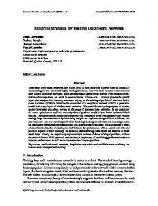
In supervised training of DNNs, the weights of the network are optimized based on a training data set. The computations during training can be divided into three main stages; forward propagation, backward propagation, and weight update. During the forward propagation, an instance from the training data set is presented to the input layer and any subsequent layer will receive a weighted sum of the outputs from all or a subset of the neurons in the previous layer. Typically a non-linear neuronal function (eg. sigmoid, tanh, ReLU etc.) is applied over this weighted sum and is propagated to the next layer. The last layer neurons’ response is compared with the dataset label and an objective function based on this observed and desired network response is minimized by altering the synaptic weights using a gradient descent algorithm. To train weights in the inner layers of the network, the gradient of the objective function with respect to the weights from the final layer needs to be back propagated based on the chain rule in differentiation. This back-propagation involves the weighted sum of an error signal from the previous layer neurons. Finally, the synaptic weight update can be determined as a product of the back-propagated errors and neuron activations. This process is repeated several times over multiple training examples to arrive at a weight distribution that enable the network to provide a satisfactory classification/detection accuracy. In Fig. 1, we introduce the mixed-precision computational memory approach for training DNNs. The most expensive operation during the forward and backward propagation is determining the weighted sum, which are matrix-vector multiplications. A computational memory unit which has resistive memory devices organized in a crossbar array is ideally suited to perform these matrix-vector operations with constant computational time complexity.9 The neuron activations of a layer, xi , are applied as voltages to the word lines using digital-to-
3
xi
Forward propagation: compute xj
W
δk
Backpropagation: compute δj
ΣkWkjδk
DAC / ADC
ΣiWjixi
ADC / DAC
Weight update: compute ΔW +
χ
-
Accumulate ΔW
pε Compute p: floor(χ /ε)
xi i
xj Wji
j δj
Wkj
k δk
p
Programming circuit
xj
= f( ΣiWji xi )
δj
= ΣkWkj δk . f'( ΣiWji xi ) (ii)
ΔWji = η δj xi
(i)
(iii)
analog converters (DACs). Currents proportional to the conductances will flow through the devices, and the resulting total current flowing through any bit line will be I j = ΣiW ji xi . Here W ji represent the device conductance connecting neuron i to a next-layer neuron j. These currents read and digitized using analog-to-digital converters (ADCs) will be the desired weighted sum operation results. The same crossbar array can be shared to perform the matrix multiplication during the back-propagation in the same layer. The errors to be back-propagated, δk , are applied as voltages to the bit lines and the currents are read out from the word lines, realizing a transposed matrix multiplication (ΣkWk j δk ). The desired weight updates are determined as the product of the back-propagated error and the neuron activation, ∆W ji = ηδ j xi , where η is the learning rate. Even though the computational memory unit can accelerate the forward and the backward propagation significantly, updating the synaptic weights with the desired precision is very challenging. Often, the devices representing the synaptic weights have a conductance update granularity dictated by the physical mechanism behind it. Let ε be the absolute value of the smallest conductance change that can be reliably achieved. Attempts to program weight updates which are much smaller could induce significant error in the training. In the proposed approach, the weight updates are accumulated in high precision in a variable χ. The device conductance will be updated only if the magnitude of the accumulated weight update becomes greater than or equal to an integer multiple of ε. The number of programming pulses, p, to be applied to the resistive memory device is
IV. EVALUATION OF THE MIXED-PRECISION ARCHITECTURE A.
The simulation framework
784 input neurons xi
250 hidden layer neurons
10 output neurons
xj xk
0 0 1 0
WJI
1
Expected image class
FIG. 1. Mixed-precision architecture based on computational memory: The synaptic weights are stored in a computational memory unit as conductance states of resistive memory devices organized in crossbar arrays. The matrix-vector multiplications associated with the forward and the backward propagation are performed in place in the memory arrays. The weight updates are accumulated in a volatile memory, χ in high precision until they become comparable to the update granularity (ε) of the memory devices. The device updates are integer multiples of ε and the same quantity will be subtracted from χ.
determined by flooring χ/ε toward zero, and the same number of εs is subtracted from the χ. Depending on the sign of p, the conductance value of the corresponding device will be increased or decreased. Note that, the actual conductance state of the devices are never read back, and hence we will never be able to confirm whether the requested weight updates are accurately attained as equivalent conductance changes in the devices. In spite of this, we show that this scheme works remarkably well and that the performance is often comparable to those of floating-point implementations. This singleshot programming method, which avoids verification and iterative programming steps, enables the acceleration of the training process. In subsequent sections, we will present a detailed evaluation of this methodology under various scenarios of device-level non-ideal behavior.
28x28 gray-scale image pixels
Computational memory unit
High-precision digital unit
WKJ
1
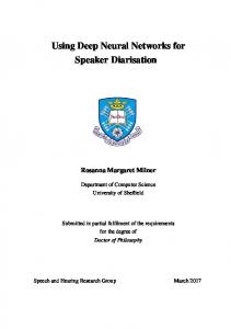
FIG. 2. Neural network for digit classification: The neural network used to evaluate the mixed-precision architecture. The objective is handwritten digit classification based on the MNIST data set. There are 784 input neurons, 250 hidden sigmoid neurons, and 10 output sigmoid neurons. The network weights are trained by optimizing a quadratic objective function using gradient descent. All the 60,000 images in the dataset are used in one epoch of training and 10,000 images for testing.
The performance of the mixed-precision architecture is analyzed based on its classification accuracy on the MNIST handwritten digit dataset using a neural network as shown schematically in Fig. 2. The number of neurons in the input, the hidden and the output layer is 784, 250, and 10 respectively. The hidden and output neurons are sigmoid. The network is trained using the entire training set of 60,000 images for ten epochs, and a test accuracy is reported based on 10,000 test images. The pixel values of the 28 × 28 gray-scale images are normalized between 0 and 1 before they are supplied as input to the network. No other preprocessing is performed on the
4
Initial weight distribution
(a) 10
6
10
4
Layer II
Count
Layer I
Count
images. We used the quadratic objective function for the backpropagation-based training and used a fixed learning rate. The network gave 98 % floating point (64-bit) test accuracy when trained using stochastic gradient descent. This classification result is used as reference to evaluate the performance of our mixed-precision approach. The final weight distribution from this high-precision training was approximately in the range [1 1].
10 2 -1
0 W JI
10
4
10 2 10 0 -1
1
0 W KJ
1
Final weight distribution Inaccuracies arising from weight-updates
Count
10 4 10 2 -1
0 W JI (c)
10 2 10 0 -1
1
0 W KJ
1
0 W KJ
1
3-bit update granularity
10 6 10 4 10 2 -1
10 4
0 W JI
1
10 4 10 2 10 0 -1
FIG. 4. Discrete weight solutions: (a) In the linear device simulations, the weights are initialized to a set of states -1, 0, and 1. (b) In non-stochastic two bit granular updates the devices go through only these discrete states and hence the update granularity also becomes the device resolution. This discrete weight solution gave a test accuracy of approximately 97%. However, in case of stochastic programming, the devices can achieve intermediate states. (c) The final weight distribution from the 3-bit update granularity simulation is also shown. The higher weight resolution improved the test accuracy by approximately 1%.
99
Test accuracy (%)
10 6
Count
In this section, we will evaluate how the proposed architecture copes with the issues associated with weight updates. We assume a hypothetical linear device with a conductance range of [-1 1] similar to the floating-point trained weight distribution. The device is assumed to have n-bit update granularity such that it covers its conductance range in 2n − 2 steps and hence it will have 2n − 1 possible levels in the absence of conductance change stochasticity. An odd number of levels was chosen to include zero. Therefore, in our mixed-precision training approach, we will update the device when the weight-update accumulation exceed the conductance change step size, ε = 2/(2n − 2). In subsequent discussions, we will use both ε and n interchangeably to indicate the granularity associated with the weight-updates.
Count
(b) 2-bit update granularity
Count
B.
98 97 96 95 94
2
4
6
8
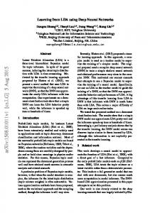
Weight update granularity (bits) FIG. 3. Effect of granularity and stochasticity associated with weight-updates: Linear devices with symmetric potentiation and depression granularity are assumed as computational memory elements. The standard deviation of the weight-update randomness, b ), is taken as a multiple of the weight-update granularity, ε. σ (∆W The error-bars indicate the standard deviation corresponding to five repetitions of the simulation. It can be seen that even in the extreme cases of highly coarse and random weight-updates, drop in the test accuracy is still within approximately 4% for 2-bit granularity.
The conductance updates in the non-volatile devices are often stochastic. Even though it is desirable to induce a change in conductance corresponding to an integer multiple of ε, the observed change is often quite different from the desired one. Therefore, the actual weight update from the device, denoted b , is modeled as a Gaussian random variable whose by ∆W
mean is ε and whose standard deviation (σ ) is a fractional multiple of ε. This device model is used as the computational memory elements representing the neural network synapses during its training using the mixed precision scheme. The devices are initialized to {-1, 0, 1} states with a discrete distribution whose variance is normalized by the number of neurons in the pre- and post-synaptic layers. Device read noise and analog-digital converters are ignored at this stage. The simulated classification accuracies with limited granularity and with different amounts of stochasticity in the updates is shown in Fig. 3. In the case where the weight updates are nonstochastic the test accuracy drop is only 1% for 2-bit, and with 3-bit granularity the accuracy is very close to that obtained in the floating-point simulation (reference). As the stochasticity increases, the performance degrades with reducing number of bits. However, it is remarkable that even though the standard deviation of the weight update is equal to or greater than the mean weight update granularity itself, drop in the test accuracy is still within approximately 4% for 2-bit granularity. The test accuracy becomes closer to the reference floating-point
Layer I
1010
1010
8-bit 6-bit 4-bit 3-bit 2-bit
108
106
104
104 5
Epoch number
Reference
108
106
0
chitecture and classification problem, 4-bit update granularity seems to offer the best case scenario of highest test accuracy with reduced programming expense.
Layer II
Reference
10
Test accuracy (%)
Number of device updates
5
0
5
10
Epoch number
FIG. 5. Sparsity associated with the devices that are being programed in the synaptic array: The device update count per epoch is plotted for different values of ε. Only a fraction of the total number of devices is programmed after each image. The number of synapses in each layer times the total training image count is indicated as reference. As the value of ε increases, the number of updates reduces by several orders of magnitude, saving significant programming overhead.
accuracy as the device granularity is further reduced. The distributions of the initial and trained weights in the two layers of the neural network for the 2-bit and 3-bit update granularity are shown in Fig. 4. The distributions are shown for non-stochastic device programming and hence the final weights are also discrete and the number of levels correspond to the update granularity. We observe that increasing the number of levels improved the classification performance until an update granularity of 4-bit beyond which the test accuracies remained approximately constant. The stochasticity associated with conductance updates helps to create a nondiscrete weight distribution. However, we found this to have no significant advantage and we typically observe a decrease in the classification performance with increasing stochasticity (Fig. 3). From the previous discussion, it can be seen that increasing the resolution of conductance change beyond a certain value does not necessarily improve the network performance. Moreover, in the mixed precision scheme, there is a significant reduction in the device programming cost with the use of larger εs. In Fig. 5, we show the number of device updates during each epoch of training. The maximum number of device updates, calculated as the product of the synapse count and the training image count, assuming all the weights are updated after each image presentation, is indicated as reference. However, in the mixed precision approach, we accumulate the updates in high precision. As a result, the smaller updates are combined and delivered together to the device. Hence, as the device update granularity (ε) increases, the devices need to be programmed less often, resulting in eventual energy savings. Programming resistive memory devices incurs significant time and power penalty and hence it is desirable to reduce the number of such programming instances, without compromising the network performance. For the chosen network ar-
99 98 97 96
2
4
6
8
Weight depression granularity (bits) FIG. 6. Effect of asymmetric conductance response: The test accuracy, when trained with devices of fixed 8-bit potentiation granularity and variable depression granularity, is plotted as a function of the depression granularity (expressed in bits). Weight updates are assumed to be deterministic. The resulting test accuracy shows less than 1% accuracy drop even in the highest asymmetric case in the simulation.
Next, we study the influence of asymmetric conductance update response. We assume a device with fixed but unequal potentiation and depression granularity. The mixed-precision method can cope with this behavior by using different thresholds, εP for conductance increment and εD for conductance decrement. For example, in Fig. 6 we assume an 8-bit potentiation granularity and the depression granularity is varied. The one bit depression in the figure correspond to a situation where the update granularity, εD , equals the entire weight range in contrast to the previous definition. The weight updates are assumed to be deterministic. The resulting test accuracies show less than 1% drop even for the maximum asymmetric case tested, demonstrating the efficacy of the proposed scheme to tolerate device update asymmetry effectively. Subsequently, we investigate the influence of non-linear conductance response. To analyze this we simulated the training problem using a device model whose non-linearity could be tuned. We chose an exponential function to model the state dependency of ∆W as suggested by Querlioz et al24 . The model essentially captures the behavior where a resistive memory device closer to the boundary conductance will exhibit smaller update compared to those away from it, when updated towards the boundary. W −W
min −β Wmax −W
bP = αe ∆W
min
max −W −β WW max −W
bD = αe ∆W
min
(1) (2)
bP and ∆W bD model the potentiation and depression Here, ∆W respectively for a device at a conductance of W . Wmin and Wmax represent the limits of the device conductance. We used the parameter β to tune the amount of non-linearity and α to adjust the update granularity. To make a reasonable comparison in training performance using models of different amount of non-linearity, we assume that two criteria have to be satisfied: the device models must have the same on-off ratio and
Potentiation
1
(b)
=0 =1 =2 =3 =4 =5
-1
Depression
-2 -1
0
1
Pulse amplitude (a.u.)
0
1 0 -1 1
-1
0
Test accuracy (%)
10
20
(c)
0
1
2
90 85
0
4
8
12
16
3
4
5
100
100
30
Pulse number
98
97
(a)
95
Read noise STD / weight range
W 99
100
0
Test accuracy (%)
(a)
W
2
Test accuracy (%)
6
(b)
90 80
DAC ADC
70 60 50
0
2
4
6
8
10
12
DAC or ADC resolution (bits) FIG. 7. Effect of non-linear conductance response: (a) Non-linear device model: the weight update (∆W ) is modeled as exponentially dependent on the current state, W . The exponential function for different amount of non-linearity is plotted. (b) Corresponding device model pulse response, where 14 potentiation pulses followed by the same number of depression pulses are applied to the device. (c) Nonlinear device model as synapse for DNN training. β = 0 correspond to a symmetric linear device and higher β values indicate increasing amount of non-linearity. Approximately 4-bit weight update granularity is assumed for the device model and mixed precision training. Weight updates were non-stochastic. The result shows that there is no significant degradation in the test accuracy even for β = 5 that corresponds to a highly non-linear conductance response.
they must take the same number of programming steps to span the whole conductance range, irrespective of the non-linearity. b versus W , and W versus pulse number responses satThe ∆W isfying these conditions for different values of β are shown in 7(a) and (b). Here, β = 0 correspond to a linear device. The number of pulses for full range potentiation or depression is assumed to be corresponding to that of a 4-bit update granularity. The same update granularity is assumed to determine the ε for the mixed precision scheme for varying amount of non-linearity. The resulting test accuracies are plotted as a function of β in Fig. 7(c). It can be seen that there is no significant degradation in the test accuracy even for β = 5, which is very close to the behavior of a binary device.
C. Inaccuracies arising from matrix-vector multiplication
In this section, we analyze the influence of conductance fluctuations and finite resolution of data converters. Resistive memory devices typically exhibit fluctuations in conductance arising from trapping/detrapping processes25 . The effect of
FIG. 8. Matrix-vector multiplication errors: (a) Effect of read noise. Gaussian distributed additive read noise is added with the computational memory devices whenever they are used for multiplication. The standard deviation (STD) of the read noise is varied as a fraction of the total device conductance range. For the mixed precision training, a 4-bit weight update granularity and non-stochastic programming is assumed. There is no significant loss in test accuracy even up to a read noise corresponding to 5% of the total weight range. (b) Effect of finite resolution data converter. The weight update granularity is assumed to be 4-bit, without stochasticity and read noise.The curve with triangle indicates simulation results where DACs are used at the crossbar input whereas the output current is read back in floating-point precision. The curve with inverted triangle indicates results where the crossbar input has floating point precision whereas ADCs are used for reading back the output current.
this read noise in the DNN training using the proposed scheme is tested by adding a zero mean white Gaussian noise to a linear device model. The noise is added to the weights whenever it is used in the matrix multiplication in the forward and the backward propagation. It is also incorporated during the testing phase (only forward propagation). The standard deviation of the noise is varied as a fraction of the total weight range. The resulting test accuracies are shown in Fig. 8a. It can seen that the methodology is quite robust to up to 5% read noise. An additional source of error in the matrix-vector multiplication is due to quantization from the DACs and ADCs. During forward propagation, the neuron activations evaluated in the digital domain are converted to analog voltages using DACs before they are applied to the word lines of the crossbar array. The weighted sum obtained as currents in the bit lines are read back using ADCs. Similarly, the back-propagated errors are converted to analog voltages when applied to the cross-bar array matrices. The range for the digital to analog converters are fixed for sigmoid and tanh neuron activations, whereas for the ReLu neurons this could be a challenge as
7 cumulative pulse response is simulated, and the statistical plot of the resulting stochastic model behavior is plotted in Fig. 9c.
PCM response Line fit 110 A
2 0
110 A 50 A
50 A
0
5
10
15
0
20
0
5
( S) G
5
10
15
Pulse number
20
Accuracy (%)
10
0
15
20
100 (d)
Training accuracy (%)
90 A
15
0
10
( S) G
20 (c)
Phase-change memory synapses
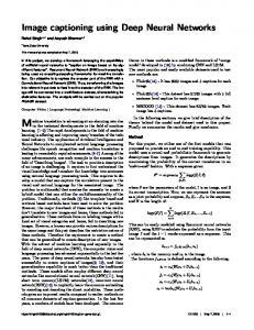
Phase-change memory is a relatively mature resistive memory technology that has found applications in the space of storage-class memory and novel computing paradigms such as neuromorphic computing26–28 and computational memory11–13 . It is based on the property of chalcogenide alloys, typically compounds of Ge, Sb and Te, which exhibit drastically different electrical resistivity depending on whether they are in the ordered crystalline phase or in the disordered amorphous phase. The crystalline phase of the Ge2 Sb2 Te5 (GST) alloy is orders of magnitude more conductive than the amorphous phase. If this material is sandwiched between two metal electrodes, the phase-configuration of the material and thus the conductance of the device can be reversibly changed by applying suitable electrical pulses. The crystalline to amorphous phase transition is accomplished by a melt-quench process and the reverse transition is governed by temperature accelerated nucleation and crystal growth29 . It is possible to achieve a continuum of conductance values by partial crystallization or amorphization in these devices. This analog storage capability makes PCM particularly suited for applications in the space of computational memory11,12 . The PCM devices exhibit most of the non-idealities we described earlier, such as limited granularity, non-linear and asymmetric conductance update, and programming stochasticity. There is also substantial read noise associated with these devices. To evaluate the suitability of PCM devices for the mixed-precision approach to train DNNs, we developed a model that captures the essential physical attributes of PCM devices. The model is created based on characterization data from approximately 10,000 devices integrated in 90 nm CMOS technology30 . The devices are subjected to 20 programming pulses of fixed amplitude and each state is read 50 times to eliminate read noise. The mean and standard deviation of the extracted conductance change (∆G) versus the average initial conductance for each programming pulse are fitted using piece-wise linear models as shown in the Fig. 9a,b. Assuming the ∆G to be a Gaussian random variable, the device
2 1
5
D.
PCM response Line fit
G
G
3
3 (b)
( S)
( S)
5 (a) 4
1
G ( S)
their range dependents on the data and weight distribution. Here, we chose sigmoid neurons for our network, which fixed the DAC range in the forward propagation. Furthermore, we normalized the back-propagated errors to fix the range for its interface converters to analog voltages. The normalization factor is multiplied with the learning rate during the weight update calculation. However, the input for the analog to digital converters are results from matrix-vector multiplications and their distribution is dependent on the number of neurons and the weight distribution in the layer. In this work, the range for ADC was determined by observing the distribution of corresponding variables representing the weighted sums. To study the effect of DACs and ADCs separately, the bit precision of one of them is varied, whereas the other variables are represented in floating-point precision. Fig. 8b shows that 8-bit resolution is sufficient to avoid a noticeable degradation in test accuracy.
95
90
Reference PCM model Read noise drop A/D drop
100 99 98 97
Training Test
0
5
10
Epoch number
FIG. 9. Training using PCM synapse models: Piece-wise linear approximations to (a) the mean (µ) and (b) the standard deviation (σ ) of the experimentally measured ∆G for Ge2 Sb2 Te5 -based PCMs for their average current conductance state (µG ) are used to model the device. (c) The resulting model conductance evolution in cumulative pulse programming. (d) Training using PCM models. Two non-linear PCM device models in differential configuration are used at the cross-points for the neural network weights. Training convergence and test accuracies (inset) are shown. Device-model based network simulation achieves 97.78% test accuracy. Additional drop from the read noise (0.26%) and analog-digital converters (0.12%) are indicated.
This device model was used to emulate the synapses in the crossbar array to study its influence on training DNNs. Two PCM devices in differential configuration with weight refresh2,31 are used. The conductance values are initialized to a normal distribution around 2 µS whose standard deviation is normalized based on the number of neurons in the pre- and post-synaptic layers. Resulting test accuracy after 10 epochs of training was 97.78% (Fig. 9d). Incorporating a fixed read noise (zero mean Gaussian noise with experimentally measured average standard deviation) and 8-bit analog-digital converters during training and testing resulted in an additional 0.38% drop in accuracy. We also tested the training performance where each synapse is realized using a single PCM device model at the crosspoint, exploiting the capability of the scheme to cope with the strongly asymmetric conductance response. The final test accuracy for the MNIST dataset classification was 96.5%, indicating the robustness of our scheme. V.
DISCUSSION
The non-volatile memory crossbar array based computational memory unit is ideally suited to perform matrix-vector
8 multiplications. By utilizing the computational memory to perform those operations when training DNNs, the forward and the backward propagation of data can be significantly accelerated. Also, the processor-memory bottleneck is reduced as the synaptic weights are not transferred during the propagations. However, the necessity to frequently update the memory devices poses an additional challenge compared to applications of computational memory where the matrix does not change11,12 . In back-propagation based training algorithm it is desirable to update the weight matrix after the presentation of each training instances. Using devices like PCM, which can attain a continuum of conductance states, it is possible to iteratively program the devices to the desired conductance states accurately32 . However, this involves repeated read/write cycles and incur significant time/power penalty. The necessity to program a large number of devices very often could overshadow the performance gain that we obtain from the in-place matrix-vector multiplication in the crossbar array. On the other end of the spectrum lies the non-von Neumann coprocessor approach proposed recently2,3,33 . As before, the synaptic weights are stored in resistive memory devices organized in crossbar arrays and the matrix-vector multiplications during forward and backward propagation are realized in place using these arrays. However, they suggest a fully parallel conductance update by overlapping pulses from the pre- and post-synaptic neuron layers. By realizing the neurons and associated circuits in place, this offers the possibility of a fully parallel non-von Neumann system. By accelerating all the three components of training DNNs, namely forward propagation, backward propagation, and weight update, this approach could be the fastest and most energy-efficient compared to alternate approaches. However, the non-idealities associated with programming the memory devices will pose significant challenges in realizing state-of the art classification accuracies. An ideal device is expected to have a symmetric weight update granularity of 10 bits3 . Experimental demonstrations using more realistic phase change memory devices have shown a limited test accuracy of less than 83%2 . Our mixed precision approach is designed to take into account the limited device update granularity seen in experimental devices today. The proposed architecture is significantly tolerant to conductance programming asymmetry and update non-linearity. In contrast to the above discussed methods, we deliver the conductance updates only when weight updates accumulated in high precision become comparable to the device update size. As a result, the number of device programming instances are reduced by several orders of magnitude as the update size increases. As a result, the advantage of matrix-vector multiplication acceleration in the data propagation stages is preserved without significant device programming overhead. We follow a blind single pulse programming approach without read-back to deliver an ε amount of update. The value of ε is chosen based on the device dynamics. The simulations show that the resulting sparse weight updates training are able to achieve classification accuracies comparable to those from the floating-point simulations in similar number of training epochs. Further, the high precision accumulation and less frequent weight-updates combined with
the inherent error tolerance of neural network training enable the architecture to cope with the high device programming stochasticity. We believe that the weight update and accumulation overhead associated with this mixed precision architecture is significantly less compared to the training acceleration we obtain. The training acceleration is achieved by computing the multiply-accumulate operation of approximately O(N 2 ) complexity in fixed time for each N × N neural network layer. The device updates are sparse and the weight update accumulation in high precision is equivalent to the weight update scheme in standard stochastic gradient decent except that the memory is initialized to zero here. The additional thresholding/flooring and subtraction operations are computationally simple and do not incur additional memory read/write operations as they can be preformed concurrently with the weight-update accumulation. Still, it is desirable to further accelerate the weight update stage of DNN training as the weight-update determination is an O(N 2 ) operation. VI.
CONCLUSION
In this work, we presented a mixed precision computing architecture to train deep neural networks. The essential idea is to use a computational memory unit in conjunction with a high precision processing unit. The computational memory unit comprises of resistive memory devices that are organized in a crossbar array. The synaptic weights are stored as conductance states of these memory devices. The computationally expensive matrix-vector multiplications arising during the forward and backward propagation stages of the backpropogation algorithm can be realized in a highly efficient manner using this computational memory unit. However, the weight updates are accumulated in high precision and are only sporadically transferred to the device array. This mixed-precision approach is shown to overcome the non-ideal behavior related to resistive memory devices such as limited granularity and stochasticity associated with their programming as well as asymmetric and non-linear conductance response. In spite of the added complexity arising from the high precision unit, we still gain in overall performance due to the substantial gain in time/power efficiency associated with the forward and backward propagation steps. Moreover, the weight updates are sparse enough to not incur a significant time/power penalty arising from the need to program the memory devices. This approach was tested using the MNIST handwritten digit classification problem and is shown to achieve remarkably high classification accuracies even with computational memory units comprising single phase-change memory devices. Realistic models of PCM devices fabricated in 90 nm technology node were used for this evaluation.
VII.
ACKNOWLEDGEMENTS
We would like to acknowledge fruitful discussions with C. Bekas, C. Malossi, G. Mariani and T. Moraitis.
9 REFERENCES
tortions. arXiv preprint arXiv:1606.01981 (2016). H. et al. ZipML: Training linear models with end-to-end low precision, and a little bit of deep learning. In Proceedings of the 34th International Conference on Machine Learning (ICML), vol. 70, 4035–4043 (PMLR, 2017). 19 Wong, H.-S. P. et al. Metal–oxide RRAM. Proceedings of the IEEE 100, 1951–1970 (2012). 20 Valov, I., Waser, R., Jameson, J. R. & Kozicki, M. N. Electrochemical metallization memories – fundamentals, applications, prospects. Nanotechnology 22, 254003 (2011). 21 Kent, A. D. & Worledge, D. C. A new spin on magnetic memories. Nature nanotechnology 10, 187–191 (2015). 22 Wong, H.-S. P. et al. Phase change memory. Proceedings of the IEEE 98, 2201–2227 (2010). 23 Nandakumar, S. R., Minvielle, M., Nagar, S., Dubourdieu, C. & Rajendran, B. A 250 mV Cu/SiO2/W memristor with half-integer quantum conductance states. Nano letters 16, 1602–1608 (2016). 24 Querlioz, D., Bichler, O. & Gamrat, C. Simulation of a memristor-based spiking neural network immune to device variations. In The 2011 International Joint Conference on Neural Networks (IJCNN), 1775–1781 (IEEE, 2011). 25 Fugazza, D., Ielmini, D., Lavizzari, S. & Lacaita, A. Distributed-PooleFrenkel modeling of anomalous resistance scaling and fluctuations in phase-change memory (PCM) devices. In IEEE International Electron Devices Meeting (IEDM), 1–4 (2009). 26 Tuma, T., Pantazi, A., Le Gallo, M., Sebastian, A. & Eleftheriou, E. Stochastic phase-change neurons. Nature Nanotechnology 11, 693–699 (2016). 27 Tuma, T., Le Gallo, M., Sebastian, A. & Eleftheriou, E. Detecting correlations using phase-change neurons and synapses. IEEE Electron Device Letters 37, 1238–1241 (2016). 28 Pantazi, A., Wo´ zniak, S., Tuma, T. & Eleftheriou, E. All-memristive neuromorphic computing with level-tuned neurons. Nanotechnology 27, 355205 (2016). 29 Sebastian, A., Le Gallo, M. & Krebs, D. Crystal growth within a phase change memory cell. Nature Communications 5, 4314 (2014). 30 Nandakumar, S. R. et al. Supervised learning in spiking neural networks with MLC PCM synapses. In 75th Annual Device Research Conference (DRC), 1–2 (IEEE, 2017). 31 Suri, M. et al. Phase change memory as synapse for ultra-dense neuromorphic systems: Application to complex visual pattern extraction. In IEEE International Electron Devices Meeting (IEDM), 4.4.1–4.4.4 (IEEE, 2011). 32 Papandreou, N. et al. Programming algorithms for multilevel phase-change memory. In IEEE International Symposium on Circuits and Systems (ISCAS), 329–332 (IEEE, 2011). 33 Kim, S., Gokmen, T., Lee, H.-M. & Haensch, W. E. Analog CMOS-based resistive processing unit for deep neural network training. arXiv preprint arXiv:1706.06620 (2017). 18 Zhang,
1 LeCun,
Y., Bengio, Y. & Hinton, G. Deep learning. Nature 521, 436–444 (2015). 2 Burr, G. W. et al. Experimental demonstration and tolerancing of a largescale neural network (165 000 synapses) using phase-change memory as the synaptic weight element. IEEE Transactions on Electron Devices 62, 3498–3507 (2015). 3 Gokmen, T. & Vlasov, Y. Acceleration of deep neural network training with resistive cross-point devices: design considerations. Frontiers in Neuroscience 10, 333 (2016). 4 Burr, G. W. et al. Neuromorphic computing using non-volatile memory. Advances in Physics: X 2, 89–124 (2017). 5 Chua, L. Resistance switching memories are memristors. Applied Physics A 102, 765–783 (2011). 6 Wong, H. S. P. & Salahuddin, S. Memory leads the way to better computing. Nature Nanotechnology 10, 191–194 (2015). 7 Boybat, I. et al. Stochastic weight updates in phase-change memory-based synapses and their influence on artificial neural networks. In 13th Conference on Ph. D. Research in Microelectronics and Electronics (PRIME), 13–16 (IEEE, 2017). 8 Seshadri, V. et al. Buddy-ram: Improving the performance and efficiency of bulk bitwise operations using DRAM. arXiv preprint arXiv:1611.09988 (2016). 9 Hu, M. et al. Dot-product engine for neuromorphic computing: programming 1T1M crossbar to accelerate matrix-vector multiplication. In 53nd ACM/EDAC/IEEE Design Automation Conference (DAC), 1–6 (IEEE, 2016). 10 Sheridan, P. M. et al. Sparse coding with memristor networks. Nature Nanotechnology 12, 784 (2017). 11 Le Gallo, M., Sebastian, A., Cherubini, G., Giefers, H. & Eleftheriou, E. Compressed sensing recovery using computational memory. In IEEE International Electron Devices Meeting (IEDM) (IEEE, 2017). 12 Le Gallo, M. et al. Mixed-precision in-memory computing. arXiv preprint arXiv:1701.04279 (2017). 13 Sebastian, A. et al. Temporal correlation detection using computational phase-change memory. Nature Communications 8 (2017). 14 Gupta, S., Agrawal, A., Gopalakrishnan, K. & Narayanan, P. Deep learning with limited numerical precision. In Proceedings of the 32nd International Conference on Machine Learning (ICML), 1737–1746 (2015). 15 Muller, L. K. & Indiveri, G. Rounding methods for neural networks with low resolution synaptic weights. arXiv preprint arXiv:1504.05767 (2015). 16 Courbariaux, M., Bengio, Y. & David, J.-P. Binaryconnect: Training deep neural networks with binary weights during propagations. In Advances in Neural Information Processing Systems, 3123–3131 (2015). 17 Merolla, P., Appuswamy, R., Arthur, J., Esser, S. K. & Modha, D. Deep neural networks are robust to weight binarization and other non-linear dis-