to paths of high camera importance. ... the camera, allowing caustic samples with higher proba- .... from S1 to S3 as 'n
Noname manuscript No. (will be inserted by the editor)
Mixing Monte Carlo and Progressive Rendering for Improved Global Illumination Ian C. Doidge · Mark W. Jones · Benjamin Mora
Received: date / Accepted: date
Abstract In this paper we seek to eliminate the noise caused by caustic paths during progressive Monte Carlo path tracing. We employ a filtering strategy over path space, handling each subspace using specialised derivations of path tracing and progressive photon mapping. Evaluating diffuse paths with path tracing allows the use of sample stratification over both pixels and the image as a whole, whilst sharp detailed caustics are produced using progressive photon mapping. This is an efficient, low noise progressive algorithm with vanishing bias combining the advantages of both Monte Carlo methods, and particle tracing. Keywords Global Illumination · Monte Carlo Integration · Path Tracing · Photon Mapping
1 Introduction Simulating global illumination efficiently is a challenging problem in computer graphics. In order to provide an effective full global illumination solution, the robust simulation of each type of light transport that occurs in a scene must be considered. Many state-of-the-art global illumination algorithms in use today find their foundations in Monte Carlo integration and the path tracing algorithm as presented by Kajiya [14]. Such methods can provide the full global illumination solution for scenes with both complex geometry and materials, making them robust under many lighting conditions. Unfortunately, path tracing suffers in the presDepartment of Computer Science, Swansea University, Swansea, United Kingdom, SA2 8PP Tel.: +44(0)1792-295393 Fax: +44(0)1792-295708 E-mail: {csiand | m.w.jones | b.mora}@swansea.ac.uk
ence of highly peaked BRDFs and in the generation of caustics from small light sources. In these scenarios, the probability of sampling the light source through specular interactions is low, resulting in high sample variance. For point light sources, direct caustics cannot be evaluated by eye paths since explicit sampling of the light source is required from a specular surface. These problems are compounded by the use of BRDF importance sampling, since specular paths with high throughput can create unpredictable peaks in the importance sampling distribution. Even after evaluating many samples, the resulting high variance shows up as high frequency noise in the image (for example Figure 1). It can be seen that filtering out the direct caustic components from the sample set provides a significant decrease in variance, at the expense of removing the important information and realism caustic paths bring to the image. Photon tracing techniques such as photon mapping can efficiently and robustly capture caustic effects with minimal high frequency noise. Such methods are consistent, but biased. Tracing paths from the light source focuses on evaluating higher radiance paths as opposed to paths of high camera importance. Whilst advantageous for caustic lighting, this removes the ability to arbitrarily distribute samples across the image to aid convergence for pixels exhibiting high variance from diffuse lighting. In many cases, this can result in some pixels converging quickly, whilst other pixels have insufficient photons and exhibit high levels of error. In this paper we seek to eliminate high frequency image noise by separating and selectively evaluating the radiance contributions at each path vertex on the fly, depending on the path characteristics. We define a set of filters over path space enabling us to treat each subpath contribution differently according to its surface interactions.
2
Ian C. Doidge et al.
(a) Full global illumination
(b) Identical samples to (a), with direct caustic contributions omitted
(c) Full global illumination, with 16x the samples of (a) and (b)
Fig. 1 The addition of caustics to a scene results in slower convergence, due to increased sample variance. (a) The full path tracing solution after 128 samples per pixel shows a significant amount of high frequency noise. (b) By evaluating the same samples but omitting just the direct caustic paths, we already see significant visual improvements with respect to Monte Carlo noise (but at the expense of losing direct caustic lighting). (c) The full global illumination solution with 2048 samples for comparison. Noise is still clearly visible in many areas
We use standard unbiased path tracing to evaluate the mainly diffuse paths, and employ an adaptation of the stochastic progressive photon mapping (SPPM) technique of Hachisuka et al. [9] to render fast crisp caustics. Despite exhibiting bias early on in rendering, we take advantage of the desirable low memory and vanishing error properties of SPPM that are commonly associated with unbiased rendering. In doing so we present the following novel contributions: • Efficiently combining path tracing and progressive photon mapping techniques to produce a vanishing error and low variance multi-pass progressive rendering algorithm. • A set of filtering criteria over path vertices are proposed, to reduce potentially high variance samples during Monte Carlo rendering using on the fly vertex contribution filtering. • Separate progressive rendering of unbiased noncaustic lighting and caustic lighting. • We demonstrate superior RMSE convergence against both standard path tracing and stochastic progressive photon mapping.
2 Related Work Particle tracing techniques allow radiance to be accumulated starting from the light source, as opposed to the camera, allowing caustic samples with higher probabilities and hence lower pixel variance. Dutre et al.’s [7] light tracing algorithm can be seen as the inverse of path tracing, making explicit connections to the image
plane at each path vertex in order to accumulate energy at each pixel. Due to this explicit connection however, many specular paths cannot be evaluated. Complex geometry and occlusion also causes problems for particle tracing methods if light sources in the scene are occluded from the visible geometry, resulting in an undesirable number of low contribution particles. For this reason techniques that use both camera importance and photon importance have been introduced. Lafortune and Willems [16] and Veach and Guibas [19] independently developed bidirectional path tracing (BDPT). BDPT independently traces paths from the camera and the light source connecting their path nodes to provide the benefits of both path and light tracing. Explicit connections between intermediate nodes of each path can also be formed in such a way as to further reduce variance [20]. Despite this, for highly specular paths BDPT performs no better than light tracing, as contributing connections between vertices cannot be made. Furthermore, due to the independence of each sample pair, there is no correlation between neighbouring pixels; a main weakness of the original path tracing algorithm. Another technique introduced by Veach and Guibas, Metropolis Light Transport (MLT) [21], generates new paths based on the mutation of a previous path, allowing correlation between pixels and favours sampling high contribution path space. This improves estimations in difficult lighting situations. Due to increased sampling of high contribution paths, often darker areas of the image are left under sampled and noisy compared to standard Monte Carlo methods. MLT also suffers
Mixing Monte Carlo and Progressive Rendering for Improved Global Illumination
in the presence of highly specular BRDFs, where even small mutations cannot effectively generate the desired low probability samples. Cline et al. [3] introduced Energy Redistribution Path Tracing (ERPT), improving upon the efficiency of MLT by adding the benefits of stratified sampling across the image. ERPT is also able to exploit pixel correlation unlike path tracing, but requires the mutation chains used for each Monte Carlo sample to be the of same length to remain unbiased. This forces the renderer to perform extra work in some areas unnecessarily and if the chains are too short, energy deposited at neighbouring pixels leads to blotchy images and low frequency noise. This effect is exacerbated by high energy caustic paths. Other unbiased rendering methods have focused specifically on improving caustics. Budge et al. [1] use a photon shooting pre-process to provide importance information to a caustic rendering pass. However this initial pre-process can be expensive and the number of photons must be chosen carefully to provide an efficient caustic lighting estimate. Furthermore, their method suffers from the same issues with low probability paths and small light sources as previous path tracing methods. DeCoro et al. [5] presented a density-based sample filtering technique that temporarily removes path contributions based on neighbourhood similarity. Although providing visible reductions in noise for their test scenes, filtering over the presence of focused caustic lighting may have a detrimental effect to the image. In addition, they filter over the radiance contributions of complete path samples, as opposed to per-vertex contributions, removing potentially low noise samples as well as those that cause high variance. Since they have more relaxed constraints, biased methods such as photon mapping [13] can generalise visibility queries, allowing them to widen path space for generating caustics at the expense of approximations. This is especially helpful for combinations of specular-diffuse-specular surface interactions, such as light sources enclosed in glass. Spencer and Jones use hierarchical photon maps to speed up caustic generation [17], and relax the photon map to reduce variance [18]. Recently Dammertz et al. [4] have introduced a biased progressive method, which also divides path space to allow for specialised algorithms to compute a solution for each subspace, in a similar fashion to our work. Although converging to a unique solution, their method is biased and does not provide physically correct results. We divide our path subspace differently to better suit the unbiased rendering techniques we employ and also provide comparisons to the stochastic
3
variant of progressive photon mapping (SPPM) which exhibits reduced aliasing and better convergence properties than the standard PPM used for comparison in their paper. Stochastic progressive photon mapping (SPPM) [9, 11] devised by Hachisuka et al. provides improvements over classic photon mapping, eliminating the need to store all previous photons, and interleaves photon shooting and distributed ray tracing passes. This allows for both a progressive reduction in bias due to the decreasing kernel radius used for photon gathering, and a theoretically unbiased progressive algorithm. PPM is effective in regions of high photon density (such as caustics) but exhibits poor convergence in low photon density regions. We leverage the properties of progressive photon mapping to provide better convergence properties caustic lighting, combining this with path tracing whose strengths lie in solving diffuse direct and indirect lighting. This allows us to produce a hybrid progressive algorithm exhibiting reduced variance and error characteristics with vanishing bias. We start with a brief overview of the original progressive photon mapping algorithm followed by an introduction to our algorithm in which we incorporate it.
2.1 Progressive Photon Mapping Progressive photon mapping is an iterative two pass algorithm that uses multiple photon maps and successively decreasing gather radii to estimate flux over the region visible through each pixel. As the kernel radius for each pixel tends towards zero, the bias vanishes resulting in a theoretically unbiased algorithm. For each pixel, a camera hitpoint is located on a visible diffuse surface, followed by the generation of a global photon map at each pass. Flux estimates are then computed at around each hitpoint using density estimation. Statistics are recorded for each pixel, including the flux estimates and kernel radius used to gather the photons. After each iteration the statistics are updated in order to reduce the kernel radius for subsequent iterations and proportionally adjust the accumulated flux. Contrary to conventional photon mapping, the photons can now be discarded leading to a low and bounded memory consumption, and a new photon map generated to produce a more refined pixel estimate over a smaller kernel radius. A single parameter α dictates the rate of radius change at each iteration i, in relation to the number of photons found within that radius Ri (S). At iteration i and for a pixel region S, we can update the total number of accumulated photons Ni (S) based on the number of new photons Mi (xi ) accumulated at the
4
Ian C. Doidge et al.
current hitpoint for this iteration xi : Ni+1 (S) = Ni (S) + αMi (xi ) s Ri+1 (S) = Ri (S)
Ni (S) + αMi (xi ) Ni (S) + Mi (xi )
(1)
(2)
As the radius is progressively reduced, the total accumulated flux over the pixel region must similarly be updated in order to maintain an accurate radiance estimate. The new flux estimate Φi (x, ω) is calculated from the current iteration photons and added to the total unnormalised flux over the pixel region. In keeping with classical photon mapping, this flux estimate can be divided by the search area πRi (S)2 , and normalised by the total number of photons accumulated so far (computed in Eqn. 1), producing a radiance estimate after each iteration. Since convergence only occurs due to the decreasing kernel radius, the parameter α provides the balance between variance and bias. In this work we offset this slower convergence by evaluating these lower density regions using path tracing, whilst taking advantage of the effectiveness of PPM in areas of high photon density.
3 Algorithm Overview Our hybrid algorithm operates in a multi-pass progressive manner, providing rapid convergence for diffuse lighting and caustic lighting independently. The first pass traces paths from the eye using standard path generation techniques, terminated by Russian roulette. Unlike path tracing, we do not yet calculate radiance contributions at each vertex. Instead we use the proceeding surface interactions to filter each vertex and classify the associated subpath into either our diffuse or caustic subspace. Radiance contributions are calculated for diffuse subpaths and added to our diffuse image buffer. Our caustic subspace is then evaluated using our modified PPM technique. Caustic photons are generated from the light sources and deposited on diffuse surfaces, terminated using Russian roulette or prematurely if they do not perform specular interactions that may contribute to our caustic subspace. A kD-Tree is constructed around the deposited photons in order to accelerate the final pass of PPM photon gathering. This pass utilises hitpoints from the initial path generation pass to gather photon flux and compute the caustic radiance estimate. After each iteration, the intermediate radiance estimates computed by the two algorithms can be combined to produce the full global illumination
solution. Maintaining a disjoint path space for each algorithm means that no bias is introduced at the compositing stage, and we require no complex or expensive weighting functions.
3.1 Path Space Separation and Filtering We draw upon regular expression notation and the path notation of Heckbert [12] in order to concisely describe our path space separation. Examples of contributions made by common paths along with their path space regular expressions are shown in Figure 2. We can apply pattern matching over these regular expressions in order to filter the paths generated by both our Monte Carlo and photon mapping techniques. We first construct an expression to encompass all paths in our caustic subspace: E(S|D)∗ D+ S + D? L
(3)
Notice firstly that this incorporates both direct and single-bounce indirect caustics due to the optional diffuse vertex, D? . Indirect caustics are also a common source of high variance in path tracing, even viewed through multiple diffuse bounces. Low probability paths generated by BRDF importance sampling at the diffuse vertex, D+ , coupled with high luminance caustic paths created by the S + L subpath can vastly increase variance, even when viewed indirectly through other diffuse vertices. Based on this caustic regular expression we can define our two path subspaces. Our camera generated path space, evaluated using path tracing, encompasses primarily diffuse paths with higher path probabilities, resulting in lower variance: (S1) ES ∗ L: Light sources viewed directly or indirectly via specular surfaces, (S2) ES ∗ D+ L: Direct and multiple bounce indirect diffuse lighting (optionally viewed via specular surfaces), (S3) ES ∗ D(S|D)∗ DDL: Indirect diffuse lighting viewed via other surface interactions. Although paths with diffuse-specular interactions are included in this subspace, potentially leading to high pixel variance, the successive diffuse vertices (...DDL) mean that these paths are of relatively low luminance. Evaluation of single and multiple bounce diffuse lighting is also performed at this stage as it responds well to sample stratification. This reduces variance and allows the application of multiple importance sampling [20] for direct lighting at diffuse vertices. The remainder of the path space is handled by our progressive photon
Mixing Monte Carlo and Progressive Rendering for Improved Global Illumination
mapping implementation, and generated from the light sources: (S4) LS + D+ (S|D)∗ E: Direct caustics, formed from the light source. (S5) LDS + D+ (S|D)∗ E: Indirect caustics, reflected from a single diffuse surface.
(a) Direct lighting and fully specular paths (ES ∗ D? L)
(b) Single bounce diffuse lighting (ES ∗ DDL)
5
surface interaction data for each path vertex. This includes the path throughput up to the current vertex, and reference to the surface’s BRDF to allow postponed radiance evaluation. A bit string is computed during path generation representing the path’s regular expression. The lower 11 bits store a binary representation of the path vertex interactions where diffuse vertices are represented by zeros and specular vertices by ones. We also encode the path length (4 bits), and whether or not the final path vertex implicitly hits a light source (1 bit). Pattern matching is applied to this bit string, and the necessary direct lighting samples at diffuse vertices and subpath radiance estimates are computed. Our filtering ensures implicit lighting from emissive surfaces is not calculated after diffuse-specular interactions (...DS ∗ L contributions) as this corresponds to direct caustic lighting. Secondly, we skip the computation of direct lighting from specular-diffuse interactions (...DS ∗ DL contributions) which correspond to indirect caustics. As can be seen in Figure 2, this allows us to reduce the noise from diffuse paths quickly relative to noise that would be introduced by caustic paths that we do not evaluate. 3.3 Caustic Evaluation
(c) Multiple bounce diffuse lighting (ES ∗ DDD+ L)
(d) Direct and Indirect caustic lighting
Fig. 2 Filtering over path traced samples allows noisy direct and indirect caustics (d) to be separated from lower variance samples (a)-(c) and more efficiently generated via photon tracing
For simplicity we will refer to our path tracing subspace from S1 to S3 as ’non-caustic’ or ’diffuse’ and the path subspace handled by the progressive photon mapping algorithm (S4 and S5) as ’caustic’. All possible paths are included in these two subspaces. This allows us to evaluate the full global illumination solution, where our two methods have no overlapping path space.
3.2 Path Tracing The first pass in each progressive iteration evaluates the image radiance from our non-caustic path subspace using Monte Carlo path tracing. In our implementation we separate the path generation from radiance evaluation to perform our added filtering step. Firstly, we generate stratified samples for BRDF sampling and trace eye paths through the scene, recording geometric and
The second pass of each iteration evaluates caustic lighting using progressive photon mapping. Having generated an eye path for each pixel, we can reuse hitpoint data from our path tracing stage to define our local visible pixel regions. The first time a diffuse hitpoint is found for each pixel, we initialise the local statistics for our progressive photon mapping, using the pixel footprint [11] to dictate the initial kernel radius. For subsequent passes these provide the points within our pixel region S around which we gather our photons. Often it is necessary to generate multiple camera paths per pixel in Monte Carlo rendering, to perform anti-aliasing as well as improved direct lighting estimates. We exploit this to enable improved initial radii values for our pixel statistics by averaging across multiple camera hitpoints, which is especially helpful in the presence of geometric discontinuities and distorted or highly anisotropic ray footprints. Having found our current hitpoints, we now need to trace and accumulate photons in order to evaluate their pixel contributions. As with our path tracing phase, we are only interested in a subset of all possible paths and so will apply our strict pattern matching on the fly during photon generation. For scenes with difficult caustic lighting, the number of caustic photons in relation to non-caustic photons may be high. This re-
6
duces the number of photons that we need to store per pass allowing faster photon gathering without loss of caustic lighting quality. Efficient photon distribution is a common problem for all photon tracing techniques and some recent solutions using adaptive and Metropolis based photon sampling can also be applied to our method [2, 8, 10]. The photon tracing stage is complete when we have deposited the desired number of caustic photons in the scene. For scenes with few or difficult to find caustic paths this can lead to excessive rejection of photons, hence we also terminate photon emission after a larger number of emissions if we have not deposited the desired amount of caustic photons.
3.4 Photon Gathering Our photon gathering phase closely resembles that of the original PPM method. For readability, we maintain similar notation to that used in the original SPPM paper. In contrast to the original algorithm, we are computing only partial radiance estimates over each pixel region using our caustic photon subset. Using the pixel hitpoints stored from the path tracing stage and corresponding shared photon statistics, we need to update the accumulated unnormalised flux over the pixel region S. For the current iteration, i, we gather the photons that are located within the sphere defined by our current local search radius Ri (S) using our kD-Tree. The updating procedure for the shared statistics remains the same as for SPPM, following Equations 1 and 2 but instead operates over our caustic subset computing the c new accumulated caustic photon count Ni+1 (S) using our caustic photons gathered in this iteration, Mic (xi ). Filtering for only caustic photons allows faster photon gathering and flux estimates to be computed over the pixel regions. This relies on the assumption of constant photon density across the gather region which is maintained in our method. Photon generation itself is unaffected by our filtering approach, and remains a purely stochastic process. This still results in a constant, non-uniform distribution of photons across the scene when averaged over many iterations, and hence a constant distribution across our visible pixel regions also. Our method operates in the same manner as PPM where the rate of radius reduction for each iteration is dependent solely on α, and we also rely on the same assumptions of constant photon density across the gather region. As with the distributed ray tracing incorporated in SPPM, our path tracing pass generates new hitpoints for each pixel at each iteration. Our Mic (xi ) photons are accumulated over a region centred around this new hitpoint xi ⊂ S. The total unnormalised flux that these
Ian C. Doidge et al.
new caustic photons in xi contribute to S is therefore: Mic (xi )
Φci (xi , ω)
=
X
fr (xi , ω, ω j ) Φj (xj , ω j )
(4)
j=1
We now update the current flux estimate for this region τi (S, ω) by multiplying it by the change in radius from Ri (S) to Ri+1 (S): τi+1 (S, ω) = (τi (S, ω) + Φci (xi , ω))
�
Ri+1 (S) Ri (S)
�2 (5)
Updating our shared statistics after each iteration ensures an increasingly accurate flux estimate is obtained over each pixel region. To produce our full global illumination image this flux estimate needs to be normalised and combined with our path tracing radiance estimate for non-caustic lighting during image reconstruction. Image Reconstruction After each iteration of the algorithm we can output our current preview of the final image by combining the pixel radiance estimates obtained from our two path subspaces. Since these subspaces evaluated by each method do not overlap, it is a trivial process of summing the radiance accumulated by the path tracing with the current progressive photon mapping estimate. The flux estimates from our shared photon statistics first need to be normalised with respect to the total number of photons emitted so far. As with our statistics updating procedure, our radiance evaluation computation is closely derived from that of SPPM. Assume that we have traced all possible photon paths (both caustic and non caustic) and separated them into our two disjoint subsets. Using our shared radius we could then gather photons that lie within xi and compute the contributing flux from each subspace independently: Mic (xi )
Φci (xi , ω) =
X
fr (xi , ω, ω j ) Φj (xj , ω j )
(6)
fr (xi , ω, ω k ) Φk (xk ω k )
(7)
j=1
Mip (xi )
Φpi (xi , ω)
=
X k=1
Where Mip (xi ) = Mi (xi ) − Mic (xi ), the number of new non-caustic photons gathered around xi . Given that we are gathering both sets of photons over the same region, our relative corrected flux values τic (S, ω) for our caustic photons and τip (S, ω) for our non-caustic photons remain proportional. After i iterations, we therefore have total of Nec (i) caustic photons and Nep (i) non-caustic
Mixing Monte Carlo and Progressive Rendering for Improved Global Illumination
7
photons. As a result our radiance evaluation can similarly be separated; τic (S, ω) L(S, ω) = lim p i→∞ (Ne (i) + Nec (i))πRi (S)2 τip (S, ω) + (Nep (i) + Nec (i))πRi (S)2 As our path tracing algorithm computes radiance values for all non-caustic lighting, we can substitute the photon mapping non-caustic radiance estimate with the unbiased path tracing estimate producing our full global illumination solution; τic (S, ω) L(S, ω) = lim p i→∞ (Ne (i) + Nec (i))πRi (S)2 Z Z + fr (x, ω, ω 0 )L(x, ω 0 )(n · ω 0 )dω 0 dx S
(a) Cornell Box
2π
4 Results and Discussion All images are rendered at 512x512 resolution on a PC with 8Gb of memory and a 2.66Ghz Intel Core i7 CPU using 8 threads. When rendering using our algorithm, we set the initial Monte Carlo rendering phase to evaluate 2 samples per pixel and the photon mapping pass to deposit a total of 50,000 caustic photons, or terminated when 400,000 photons have been emitted. This provides us with a good balance between the convergence of caustic and diffuse lighting for our test scenes, as well as optimising the use of the hitpoint data generated in the path tracing pass. Table 2 shows the distribution of work. Our first test scene (Figure 4) is a Cornell Box scene containing glass and chrome spheres, which produce a wide variety of caustic lighting from an area light source. High frequency noise in the path tracing image is very apparent and obscures details in the image. Using our method dominant high frequency noise is removed, and far better clarity is visible in all areas of Caustic Paths Photons Direct Indirect Deposited Emitted
Scene Cornell PT Box Ours
153k (122k)
218k (172k)
4.71mil
52.2mil
Ring
PT Ours
1328 (1069)
12.8k (10.1k)
5.40mil
37.7mil
Shapes
PT Ours
16.7k (12.3k)
10.0k (7.31k)
6.22mil
81.1mil
Table 1 Comparison of the number of caustic paths generated using path tracing and our method. Our filtered photon mapping pass evaluates many times more caustic samples, than path tracing. The first two columns for our method (in brackets) show the number of radiance contributions excluded by our path filtering. Both algorithms were run for 5 minutes
(b) Ring
(c) Shapes Fig. 3 Graph plots of the log root mean squared error versus time for our three test scenes. Our hybrid method provides consistently lower error for all our scenes, and the order of convergence is dependant on the balance of diffuse and caustic lighting in the scene
the image. Since we show equal time comparisons, the number of diffuse samples evaluated by our method is reduced due to the additional time required for photon mapping. Despite this, regions of diffuse lighting have not noticeably suffered, due to the elimination of high frequency noise by our path filtering. In comparison to SPPM, our algorithm exhibits far less noise from
8
Ian C. Doidge et al.
Path Tracing
Our Method
SPPM
Converged Path Tracing
Fig. 4 Path tracing is effected by its poor evaluation of caustic paths compared to our method, without introducing the lower frequency noise produced by SPPM visible around the image edges, or the higher frequency noise on the back wall and glass ball. Images for all three methods were rendered in 30 minutes Scene
Iterations Path Tracing Photon Generation Photon Gather Image Reconstruction
Cornell Box Our Method (30mins) PT SPPM
820 2034 1282
1413s 1802s 188s
289s 280s
70.45s 1313s
28.28s 21.4s
Ring (30 mins)
Our Method PT SPPM
586 1446 929
1413s 1800s 370s
324.7s 721s
51.45s 689s
12.43s 11.45s
Shapes (4 mins)
Our Method PT SPPM
170 458 186
139.2s 240.30s 63.52s
56.3s 80.62s
32.21s 92.0s
5.05s 4.85s
Table 2 Time spent in each of the main stages of our algorithm with reference to path tracing and SPPM, in order to produce the images shown in this section. Note that each iteration of our method evaluates two Monte Carlo paths, and gathers photons around one hitpoint. Path Tracing times for our method include the path generation, regular expression filtering and diffuse radiance calculations. For SPPM it represents the time spent in the distributed ray tracing passes
Path Tracing
Our Method
SPPM
Converged Path Tracing
Fig. 5 Equal time comparison after 30 minutes between path tracing, our method and SPPM. A low noise path tracing image is also provided for reference, which took many hours to render. Close ups of the same images show reductions in noise for our method compared to both methods
diffusely lit regions, whilst producing caustics of equivalent quality. Figure 5 shows results from our Ring scene, a metal ring on a flat surface in a walled environment lit by a small area light source. Path tracing cannot effectively render the cardioid caustic due to the small difficult to sample light source, resulting in an initial increase in image error (Figure 3(b)). SPPM has noticeable noise as a result of low photon densities on the wooden floor
and bricked walls. Our method evaluates all light paths effectively, producing diffuse lighting with similar quality to the path tracing image, and caustics comparable to those produced by SPPM. Finally, we present a scenario that can be challenging for both camera path and light tracing methods (Figure 6). Due to its open nature, particle tracing techniques perform poorly, allowing many emitted photons to miss the geometry entirely or be deposited in regions with low camera importance.
Mixing Monte Carlo and Progressive Rendering for Improved Global Illumination
Path Tracing
Our Method
SPPM
9
Converged Path Tracing
Fig. 6 Equal time comparison after 4 minutes of rendering between path tracing, our method and SPPM. This scene displays both direct and indirect lighting, in addition to a range of reflected and refracted light paths. Due to its open nature, both the indirect diffuse lighting on the blue box, and the caustic lighting seen via reflection and refraction are difficult to evaluate
An area light source illuminates a large plane containing diffuse, glass, and reflective objects. Caustics are visible directly as well as via reflections and transmission, thus also posing a challenge for path tracing techniques. Interestingly, path tracing provides lower overall error for this scene than SPPM due to the wide dispersion of photons traced from the light source. Even with the similar photon distribution, the direct light at diffuse vertices provides vast improvements. Computing RMSE values for our three scenes further demonstrates the effectiveness of our approach. Where diffuse lighting presents more of a challenge (such as the Cornell Box scene), convergence for our method follows that of path tracing. In scenes dominated by caustics, where path tracing struggles (Ring scene), our method resembles the convergence rates of SPPM. In more mixed environments such as our last scene, both the caustic and diffuse lighting converge at similar rates, with neither of our two methods consistently dominating the rate of convergence. 5 Conclusions and Future Work Achieving high efficiency whilst maintaining robustness is a desirable but difficult to attain property for computer graphics algorithms. It has been shown that a single specific algorithm can often solve a particular light transport problem more efficiently than a generalised one [4,6,15]. We have presented a novel multi-pass progressive algorithm that combines the benefits of both Monte Carlo path based based and progressive photon based methods via path space filtering. Though separable path space filtering methods have been used before for full global illumination [1, 4], our algorithm has the advantage of being both progressive and physically based, allowing convergence to the correct solution or until the desirable level of quality is achieved. Our algorithm represents a concept that is equally applicable
to any Monte Carlo based method such as bidirectional path tracing or Metropolis light transport. A desirable addition would be to allow the automatic adjustment of Monte Carlo and photon paths during rendering, improving convergence for scenes with difficult caustic or diffuse lighting. Care would need to be taken however to ensure that portions of path space were not under sampled prematurely, which could yield higher variance than has yet been identified. Acknowledgements The work presented in this paper was funded by an EPSRC doctoral training grant and also EPSRC grant number EP/I031243/1. We would like to be notified about any adoption of this method into ray-tracing software since our funding council seeks to record the impact of its funded research.
References 1. Budge, B.C., Anderson, J.C., Joy, K.I.: Caustic forecasting: Unbiased estimation of caustic lighting for global illumination. Comput. Graph. Forum 27(7), 1963–1970 (2008) 2. Chen, J., Wang, B., Yong, J.H.: Improved stochastic progressive photon mapping with metropolis sampling. Computer Graphics Forum 30(4), 1205–1213 (2011) 3. Cline, D., Talbot, J., Egbert, P.: Energy redistribution path tracing. ACM Trans. Graph. 24(3), 1186–1195 (2005) 4. Dammertz, H., Keller, A., Lensch, H.P.A.: Progressive point-light-based global illumination. Computer Graphics Forum 29(8), 2504–2515 (2010) 5. DeCoro, C., Weyrich, T., Rusinkiewicz, S.: Density-based outlier rejection in monte carlo rendering. Computer Graphics Forum (Proc. Pacific Graphics) 29(7), 2119– 2125 (2010) 6. Donikian, M., Walter, B., Bala, K., Fernandez, S., Greenberg, D.P.: Accurate direct illumination using iterative adaptive sampling. IEEE Transactions on Visualization and Computer Graphics 12, 353–364 (2006) 7. Dutr´ e, P., Lafortune, E.P., Willems, Y.: Monte Carlo light tracing with direct computation of pixel intensities. In: 3rd International Conference on Computational Graphics and Visualisation Techniques,, pp. 128– 137 (1993)
10 8. Fan, S., Chenney, S., Lai, Y.C.: Metropolis Photon Sampling with Optional User Guidance. In: Proceedings of the 16th Eurographics Symposium on Rendering, pp. 127–138. Eurographics Association (2005) 9. Hachisuka, T., Jensen, H.W.: Stochastic progressive photon mapping. ACM Trans. Graph. 28(5), 141:1–141:8 (2009) 10. Hachisuka, T., Jensen, H.W.: Robust adaptive photon tracing using photon path visibility. ACM Trans. Graph. 30(5), 114:1–114:11 (2011) 11. Hachisuka, T., Ogaki, S., Jensen, H.W.: Progressive photon mapping. ACM Trans. Graph. 27(5), 130:1–130:8 (2008) 12. Heckbert, P.S.: Adaptive radiosity textures for bidirectional ray tracing. In: Proceedings of the 17th annual conference on Computer graphics and interactive techniques, SIGGRAPH ’90, pp. 145–154. ACM, New York, NY, USA (1990) 13. Jensen, H.W.: Global illumination using photon maps. In: Proceedings of the eurographics workshop on Rendering techniques ’96, pp. 21–30. Springer-Verlag, London, UK (1996) 14. Kajiya, J.T.: The rendering equation. In: Proceedings of the 13th annual conference on Computer graphics and interactive techniques, SIGGRAPH ’86, pp. 143–150. ACM, New York, NY, USA (1986) 15. Kollig, T., Keller, A.: Illumination in the Presence of Weak Singularities. In: Monte Carlo and Quasi-Monte Carlo Methods (2004) 16. Lafortune, E.P., Willems, Y.D.: Bi-Directional Path Tracing. In: Proceedings of the International Conference on Computational Graphics and Visualization Techniques (COMPUGRAPHICS ’93), pp. 145–153 (1993) 17. Spencer, B., Jones, M.W.: Hierarchical photon mapping. IEEE Transactions on Visualization and Computer Graphics 15(1), 49–61 (2009) 18. Spencer, B., Jones, M.W.: Into the blue: Better caustics through photon relaxation. Eurographics 2009, Computer Graphics Forum 28(2), 319–328 (2009) 19. Veach, E., Guibas, L.: Bidirectional estimators for light transport. In: Proceedings of the Eurographics Workshop on Rendering, pp. 147–162. Eurographics (1994) 20. Veach, E., Guibas, L.J.: Optimally combining sampling techniques for monte carlo rendering. In: Proceedings of the 22nd annual conference on Computer graphics and interactive techniques, SIGGRAPH ’95, pp. 419–428. ACM, New York, NY, USA (1995) 21. Veach, E., Guibas, L.J.: Metropolis Light Transport. In: Proceedings of the 24th annual conference on Computer graphics and interactive techniques, SIGGRAPH ’97, pp. 65–76. ACM, New York, NY, USA (1997)
Ian C. Doidge et al.