MIXING PERFORMANCE OF VISCOELASTIC ...

MIXING PERFORMANCE OF VISCOELASTIC FLUIDS IN A KENICS KM IN-LINE STATIC MIXER J. Ramsaya, M.J.H Simmonsa1, A. Ingrama, E.H. Stittb a

School of Chemical Engineering, University of Birmingham, B15 2TT, UK; b

Johnson Matthey Technology Centre, Billingham, TS23 1LB, UK

Abstract The mixing of ideal viscoelastic (Boger) fluids within a Kenics KM static mixer has been assessed by the analysis of images obtained by Planar Laser Induced Fluorescence (PLIF). The effect of fluid elasticity and fluid superficial velocity has been investigated, with mixing performance quantified using the traditional measure of coefficient of variance CoV alongside the areal method developed by Alberini et al. (2013). As previously reported for non-Newtonian shear thinning fluids, trends in the coefficient of variance follow no set pattern, whilst areal analysis has shown that the >90% mixed fraction (i.e. portion of the flow that is within ±10% of the perfectly mixed concentration) decreases as fluid elasticity increases. Further, the >90% mixed fraction does not collapse onto a single curve with traditional dimensionless parameters such as Reynolds number Re and Weissenberg number Wi, and thus a generalised Reynolds number Reg = Re/(1+2Wi) has been implemented with data showing a good correlation to this parameter.

Highlights 

Kenics KM static mixer shows poor mixing performance with viscoelastic fluids



Viscoelastic fluids show greater pressure drop across mixer than predicted



Significant time variation in mixing quality at mixer outlet



Mixing quality correlates to generalised Reynolds number Reg = Re/(1+2Wi)

Keywords Mixing performance; Kenics; static mixer; PLIF; viscoelasticity; fluid blending

1

Corresponding author: Professor M.J.H. Simmons, School of Chemical Engineering, University of Birmingham, B15 2TT, UK; Email: [email protected]; Tel: 0121 414 5371

Page 1 of 35

1. Introduction

The formulation of complex fluid products in industrial processes offers many challenges. Many common multiphase products, such as paints, inks or ceramic pastes, possess high levels of particulate solids loading, typically 45 to 55 % by volume. Under shear conditions particle jamming can often occur, leading to highly viscous or viscoelastic rheologies. Due to the highly viscous consistency of these fluids, industrial blending operations take place under laminar flow conditions presenting significant challenges in achieving product homogeneity.

The primary complexity in material processing stems from the highly non-linear rheological behaviour these complex multiphase systems possess, manifesting as viscoelastic flow effects which, in addition to the high solid phase volume, can be attributed to polymer content in the liquid matrix and other multiphase components such as droplets and bubbles1.

The interaction between

viscoelasticity and continuous flow processes has received comparatively little attention in the open literature as most studies have focussed on batch stirred tank systems. Traditionally, these stirred tanks have been agitated using specialised impeller designs such as the anchor, helical ribbon 2-5 or butterfly impeller6 in order to perform the required mixing duty with viscoelastic fluids. However, batch systems possess many limitations, such as high energy demands and high labour costs due to operator intervention and process cleaning. It is therefore imperative to shift to continuous methods of processing, owing to their comparative reduced energy input and labour, smaller plant footprint enabling a greater degree of process intensification, and the ability for tighter process control allowing for a more consistent product output7.

In recent years there has been significant interest in the performance of in-line static mixers, also known as motionless mixers, in both laminar and turbulent flow applications. Static mixers consist of metallic inserts that fit into a pipeline and redirect flow in order to improve inter-material contact, which is beneficial in mixing systems ranging from simple blending operations through to chemical reaction and heat transfer7.

Implementation of these mixers into process lines is relatively

straightforward: only standard pumping equipment is required for use as the mixer inserts into a pipeline although there will be an inevitable increase in pressure drop. Although many manufacturers offer a range of designs tailored to each application, the most common type under investigation in academic circles is the Kenics KM mixer (Chemineer, USA) which is comprised of a series of helically twisted elements. The simplicity of this mixer design has made it a favoured geometry for investigation, as its split-and-recombine design performs the standard Baker’s transformation for mixing duties in laminar flow7. Furthermore, the geometry is easily modelled in computational fluid dynamics (CFD) simulations, and has been the subject of several investigations with the aim of assessing flow structures within the mixer itself8-14. Page 2 of 35

Some of the earliest investigations into static mixer performance by Shah & Kale 15 and Chandra & Kale16 focussed exclusively on the pressure drop across the mixer with various fluids. Remarkably, despite limited literature on static mixer performance available at the time, viscoelasticity was also investigated. They found a significant increase in pressure drop as fluid elasticity increased at low Reynolds numbers with data fitting a polynomial type expression. Further, additional works17;18 have also attempted to fit pressure drop data to a variety of models, with some19 applying a stirred tank analogy using a power factor Kp in laminar flow. The design factor KL, also known as the z-factor, is the most commonly used measure for mixer pressure drop ratio, and is defined as:

𝐾𝐿 =

𝑓𝐷,𝑚𝑖𝑥𝑒𝑟 𝑓𝐷,𝑒𝑚𝑝𝑡𝑦 𝑝𝑖𝑝𝑒

=

Δ𝑃𝑚𝑖𝑥𝑒𝑟 Δ𝑃𝑒𝑚𝑝𝑡𝑦 𝑝𝑖𝑝𝑒

(1)

Where fD is the Darcy friction factor and ΔP the pressure drop. For the Kenics KM mixer, KL is commonly taken as 6.9, a value determined for Newtonian fluids in laminar flow7;20. Other work has suggested that for non-Newtonian fluids the value of KL is significantly lower than this21, and furthermore the presence of viscoelasticity may well produce significant deviation from this design parameter due to the existence of secondary flows perpendicular to the main flow direction; previous design parameters have been calculated based on the laminar flow of Newtonian fluids only.

Assessing the impact of viscoelasticity on processes possesses many challenges. Owing to their nonlinear behaviour, it is often difficult to define a single parameter to fully characterise flow behaviour. Most studies apply traditional approaches, with correlations of Reynolds number, Re, and viscoelastic Weissenberg number, Wi, however these in isolation cannot fully describe the flow conditions as they ignore the relative effects of elasticity and inertia respectively. Some studies have implemented a combined approach, using dimensionless groups such as the Elasticity number El22;23, or more recently the generalised Reynolds number Reg, which seeks to correct the viscous stress term present within the Reynolds number for elastic effects24. All of these recent studies applied optical flow measurement techniques such as Particle Image Velocimetry (PIV)25-31, Planar Laser-Induced Fluorescence (PLIF)32-36 or dye decolourisation techniques37;38 and were focussed on viscoelastic mixing behaviour in stirred tanks; to date there have been very few publications investigating viscoelastic fluids within static mixers16;17. These optical methods all require transparent fluids which can be a limitation, however another non-invasive technique, Positron Emission Particle Tracking (PEPT) which is suitable for opaque fluids, has also been applied to static mixers for Newtonian and non-Newtonian inelastic fluids39. The technique reveals velocity fields and shear rates in addition to mixing measures such as segregation index40. For local mixing performance, PLIF has become the experimental method of choice for a range of mixing applications. The mixing region is Page 3 of 35

illuminated with a laser sheet perpendicular to the camera: the fluorescent intensity of a dye (injected into one of the mixing phases) is used to infer a map of the instantaneous and transient concentration field.

Most of these techniques have assessed mixing performance using the traditional method of intensity of segregation, as determined by the coefficient of variance CoV within the flow. However, recent studies41 have shown CoV to be insufficient in describing the complete mixing condition of a fluid as it does not include the scale of segregation, the other of the two primary measures of mixing stated by Danckwerts42. In order to address this deficiency, Alberini et al.21 developed the areal distribution method which combines scale and intensity of segregation in a frequency distribution of mixedness. Originally developed for static mixer geometries, the technique has also been applied to stirred tanks43.

Although there has been much investigation into characterising viscoelastic fluids, understanding the application of these fluids in processes remains difficult. For example, the literature is divided as to whether secondary flows, generated due to normal stress differences present only in viscoelastic flow, enhance or inhibit mixing performance: several works argue that the additional transport in the nonprimary flow direction aids convective mixing processes and thus improves performance 31;38;44, whilst others claim that the same transport reduces this performance due to the solid-like portions of the flow being less readily mixed6;23;45.

As the viscoelasticity of multiphase fluids remains poorly

characterised and its effect on processes is still unknown due to the complexity of decoupling viscous and elastic effects, it is desirable to investigate a more idealised viscoelastic fluid to understand the underlying flow phenomena. More specifically, it is necessary to isolate the well-documented effect of varying viscosity from the little understood effect of varying elasticity, which is achieved by using a class of viscoelastic fluid known as the “Boger” fluid, typically made from the addition of a dilute polymer to a Newtonian solvent46;47. These fluids possess a constant viscosity and an elasticity that can be controlled through varying polymer concentration. They also have the benefit of being optically transparent and have been used in several flow visualisation investigations 48-51. As the fluid viscosity and elasticity of Boger fluids can be controlled independently they are suitable candidates for mimicking a range of other more complex materials6.

This work seeks to characterise the interaction between viscoelastic materials and continuous in-line static mixers through assessment of blending performance and energy efficiency. Qualitative and quantitative mixing performance has been obtained using PLIF measurements, whilst pressure drop measurements enable calculation of energy input. Mixer behaviour has been examined using fluids of increasing rheological complexity through use of transparent Newtonian and Boger fluids with the same base fluid viscosity. Key performance parameters such final mixing quality assessed through Page 4 of 35

areal analysis and coefficients of variance (CoV) have been calculated over a range of industrially relevant process conditions and compared to a range of dimensionless hydrodynamic parameters and process energy inputs in order to determine the underlying controlling mechanisms for mixing performance.

2. Methods & Materials

2.1 Experimental Set-up

Experiments were performed in a continuous flow rig as displayed in Figure 1. The main flow into a 12.5 mm ID pipe was delivered from a 20 L header tank via a gear pump (Liquiflow) powered by a motor drive (Excal Meliamex Ltd.). A secondary flow stream dyed with 0.5 mg L-1 Rhodamine-6G (Sigma Aldrich, UK), which acts a passive scalar for local concentration measurement, was delivered from a pressurised 5 L vessel via a gear pump (GB-P35, Cole-Parmer, UK).

Flowrates were

measured from an in-line flowmeter (Krone) in the main flow and indirectly from pump speed via previous calibration measurements for the secondary stream. The secondary stream was injected via a coaxial nozzle, 4 mm I.D., at a flow ratio of 10% of the total stream flowrate in order to achieve isokinetic conditions between the main and secondary streams. The combined stream then passed through a six element ½” (internal diameter 14.7 mm) diameter Kenics KM static mixer (Kenics, USA), with all six elements at 90° to the preceding element. Downstream of the mixer outlet was a transparent pipe section, consisting of a ½” I.D. unplasticised poly(vinyl chloride) (uPVC) pipe encased in a transparent poly(methyl methacrylate) square-section box filled with water. At the exit of the transparent section a tee-piece was fitted, with the branching outlet dumping to the fluid drain whilst the other outlet was capped with a poly(methyl methacrylate) viewing window permitting observation of the upstream pipe cross-section when illuminated with laser light. Pressure drop measurements were taken ex-situ through fitting 1 bar Keller S35X pressure transducers (Keller, UK) at the mixer inlet and outlet. The flowrates Q of 68.4 to 136.8 L hr-1 implemented in this study are typical of industrial processing superficial velocities for the pipe diameters studied. Reynolds number fall well below the critical value of Re = 2 100, with values of Re < 30 existing in all cases. Table 1 displays the experimental conditions.

Page 5 of 35

Figure 1: a) Equipment set-up diagram; b) static mixer section dimensions

Table 1: Experimental conditions for PLIF experiments Main stream

Secondary

Total

Superficial

Newtonian

Newtonian

flowrate Q

stream

flowrate QT =

velocity u

mixer wall

Reynolds

(L hr-1)

flowrate QS

Q + QS

(m s-1)

shear rate 𝜸̇ 𝑾

number Re

(L hr-1)

(L hr-1)

(s-1)

(dimensionless)

61.6

6.8

68.4

0.15

331

14.5

82.1

9.1

91.2

0.20

441

19.4

123.1

13.7

136.8

0.30

661

29.0

2.2 Fluid Rheology

A class of transparent viscoelastic fluids known as Boger fluids were used in this study in order to provide viscosities and elasticities in a similar range to industrially relevant viscoelastic materials. Fluids were formulated using a bench-top laboratory mixer (Heidolph RZR-2102, Heidolph UK). Dilute polymer solutions of poly(acrylamide) (Sigma Aldrich, UK) in aqueous glycerol (ReAgent,

Page 6 of 35

UK) were formulated in 20 L batches, with water used to make up the remainder. Sodium chloride salt (Sigma Aldrich, UK) was added to aid polymer dissolution during fluid formulation. Rheological characterisation was performed using a Discovery Hybrid HR-2 rheometer (TA Instruments, USA) using a 40 mm 4° cone and plate geometry over a range of shear rates, 𝛾̇ , between 0.1 and 1000 s-1. This shear rate range was selected to capture the maximum theoretical shear rate (found at the pipe wall) for the static mixer at experimental conditions using the design correlation:

𝛾̇ 𝑊 =

𝐾𝐺 𝑢 𝐷

(2)

Where KG is the mixer shear rate coefficient (28 for a Kenics KM)7, u the superficial flow velocity (m s-1) and D the mixer diameter (m).

Normal stress differences, the differences in the principal normal stress components of the stress tensor52, were directly measured during the acquisition of shear stress versus shear rate data on the same instrument through axial force measurement. The fluid relaxation time, , the primary measure of material viscoelasticity, was calculated as a function of shear rate from the ratio of first normal stress difference N1 to viscosity and fitted to a power law model23:

𝜆(𝛾̇ ) =

𝜓1 (𝛾̇ ) 2𝜂(𝛾̇ )

=

1 𝑁 (𝛾̇ ) ( 12 ) 2𝜂(𝛾̇ ) 𝛾̇

𝜆 = 𝑎𝛾̇ 𝑏

(3)

(4)

Where ψ1 is the first normal stress coefficient, η the fluid apparent viscosity, N1 the first normal stress difference, 𝛾̇ the shear rate, while a and b are constants. The compositions of the model fluids used and their rheological parameters can be found in Table 2. Figure 2 displays the rheological data obtained.

Page 7 of 35

Figure 2: a) Shear stress τ and viscosity η versus shear rate 𝛾̇ for Boger fluid (viscosity scale linear); b) First normal stress differences N1 and relaxation times λ for Boger fluids Table 2: Fluid compositions and rheological parameters

Glycerol Polyacrylamide (wt. %)

Boger A -

Page 8 of 35

Boger B 0.01

0.02

Glycerol (wt. %)

90.00

90.00

90.00

Water (wt. %)

10.00

8.33

8.32

-

1.66

1.66

Sodium chloride (wt. %)

Fluid

Viscosity 𝜼 (Pa.s)

Relaxation time pre-

Relaxation time power

exponential factor a (sb+1)

law exponent b (-)

Glycerol

0.188 (±0.014)

-

-

Boger A

0.195 (±0.019)

87.76 (±18.49)

-1.81 (±0.02)

Boger B

0.164 (±0.024)

157.36 (±31.12)

-1.78 (±0.04)

As Figure 2a shows, both Boger fluids possess approximately constant viscosity across the measured range. Additionally, these values are similar, indicating that glycerol concentration controls the baseline material viscosity and thus allows us to assess elasticity independently. The elastic responses are shown in Figure 2b; for both materials N1 increases with increasing shear rate, however the rate of increase reduces at increasing shear rates indicating that instead of the expected quadratic N1 response that a “true” Boger fluid should possess, which is only valid at low shear rates, a power-law type model is more suitable. However, it can be seen that at all measured values the response of Boger A displays lower values of N1, thus indicating that Boger A possess a lower elasticity than Boger B; this is further observed in the fluid relaxation times which also fit a power law model.

At the experimental conditions used for both PLIF and pressure drop experiments, experimental Reynolds numbers Re vary between 10 and 30 and are defined as:

𝑅𝑒 =

𝜌𝑢𝐷 𝜂

(5)

Where ρ is the fluid density, with actual values of superficial velocity and measured internal diameter used in this calculation.

Additionally, the fluid elasticity has been calculated through calculation of the dimensionless Weissenberg number Wi, which is defined as the ratio between the material and process characteristic timescales at steady state. The value has been calculated by: 𝑊𝑖 = 𝜆𝛾̇ 𝑊

Page 9 of 35

(6)

Where λ is the material relaxation time. This can also be coupled to the Reynolds number in order to provide an overall dimensionless parameter to describe the flow.

A commonly implemented

definition is that of the Elasticity number El, which is defined as the ratio between elastic and inertial forces within the flow:

𝐸𝑙 =

𝑊𝑖 𝑅𝑒

(7)

Further, Bertrand et al.24 have proposed a new method for a combined approach, through implementing a generalised Reynolds number Reg. This aims to account for fluid elasticity through correcting the viscous term in the Reynolds number definition, such that: 𝑅𝑒𝑔 = 𝑅𝑒(1 + 2𝑊𝑖)−1

(8)

For an elastic fluid, the value of Reg is always lower than the standard definition of Re for Wi > 0. In the Newtonian case (Wi = 0), Reg = Re. This approach can only be applied to second-order fluids such as Boger fluids, as this definition of Reg relies on a second-order stress response. The derivation of Reg is shown in Appendix A.

2.3 Power Input

Process power input was determined from pressure drop measurements over a range of fluid velocities. Specific energy input at a given flow condition is given by:

𝜀=

Δ𝑃 𝜌

(9)

Where ε is the specific energy input (J kg-1) and ΔP the pressure drop (Pa).

In laminar flow, the theoretical empty pipe pressure drop is calculated from the Hagen-Poiseuille equation:

Δ𝑃𝑒𝑚𝑝𝑡𝑦 𝑝𝑖𝑝𝑒,𝑡ℎ𝑒𝑜𝑟𝑒𝑡𝑖𝑐𝑎𝑙 =

128𝜂𝐿𝑄 𝜋𝐷 4

=

32𝜂𝐿𝑢 𝐷2

(10)

Where L is the length of the measurement section (m). Further, the empty pipe Darcy friction factor fD can be calculated by:

Page 10 of 35

𝑓𝐷 =

64 𝑅𝑒

=

Δ𝑃 𝐿 𝐷

(11)

1 2

( )( 𝜌𝑢2 )

Mixer friction factor and pressure drop ratio KL have been calculated according to equation (1). Both the standard Reynolds number definition and the generalised Reynolds number shown in equation (8) have been implemented in order to assess deviation from the predicted pressure drop values.

2.4 Planar Laser Induced Fluorescence (PLIF)

PLIF was performed at all experimental conditions (Table 1).

A 532 nm Nd-YAG laser

(nanoPIV, Litron, UK) operating at 2.07 Hz was fitted with -100 mm cylindrical lens and a 500 mm focussing lens in order to project a planar sheet, of thickness less than 0.1 mm, through the transparent mixer outlet section. A 12-bit 4MP CCD camera (TSI, USA) captured images synchronous to the laser pulses, with timings controlled via a synchroniser (TSI 610035) linked to a personal computer operating Insight 4G software for image acquisition (TSI, USA).

The image resolution was

22 μm pixel-1, hence all measurements of mixing performance assess the macromixing quality only. 20 images were recorded at all conditions equating to 9.67 seconds of imaging, which is of the order of several fluid relaxation times at all conditions.

Rhodamine-6G was added to the secondary flow stream as the fluorescent tracer. A 545 nm cut-off lens was fitted to the camera to act a high-pass filter, eliminating all light but that fluoresced by the dye (λ = 560 nm).

In order to select a suitable concentration of fluorescent dye, calibration

experiments were performed by filling the pipe section with dye of a set concentration. An example calibration curve is displayed in Figure 3; it was observed that the local greyscale values did not vary significantly across the image and therefore a single average greyscale has been used to construct the greyscale-concentration relationship.

As the relationship between greyscale value and dye

concentration is linear below a critical dye concentration, it is possible to calculate local concentrations and thus mixing performance.

Page 11 of 35

Figure 3: Example PLIF calibration curve of rhodamine-6G concentration against average image greyscale value

From PLIF data, areal concentration distributions are calculated using bespoke MATLAB code. The method is explained in full in Alberini et al.21; only an abridged version is presented here for brevity. The perfectly mixed concentration (or grayscale) value 𝐶̅ is calculated from a theoretical mass balance across the mixer. Using the principle that material that is mixed to an arbitrary degree, X, will possess ̅̅̅ , it is possible to split the observed concentrations in the range of [1 − (1 − 𝑋)]𝐶̅ to [1 + (1 − 𝑋)]𝐶 images into regions of known mixedness, e.g. 80 to 90 % mixed, 50 to 60 %, > 90 % etc.

The

MATLAB DipImage toolbox (Delft University of Technology, The Netherlands) is implemented to isolate regions of the image within the same concentration range, and the number of pixels within each concentration is summed to give the fraction fX of the image in the given mixedness quality range.

Additionally, in order to provide a comparison to the standard mixing measurements, the coefficient of variance CoV for the image is calculated. 𝐶𝑜𝑉 =

𝜎 𝐶̅

(12)

Where σ is the local concentration variance (g L-1) and 𝐶̅ is the perfectly mixed concentration (g L-1). The variance is calculated by:

Page 12 of 35

𝜎=

1 ∑𝑛 (𝐶 ′ 1−𝑛 𝑖=0 𝑎,𝑖

2

− 1)

(13)

Where n is the maximum number of data points (in this case the total number of locations), and C’a,i is defined as: ′ 𝐶𝑎,𝑖 =

𝐶𝑎,𝑖 −𝐶0 𝐶̅ −𝐶0

(14)

Where Ca,i’ is the normalised concentration of component a at location i, Ca,i is the concentration at location i, and C0 and 𝐶̅ the initial and fully-mixed conditions respectively. With respect to the timescales involved, time t = 0 s was arbitrarily determined as the time that the first image was acquired at a given flow condition.

The coefficient of variance can be normalised to a reduced coefficient of variance CoVr, which displays the reduction in CoV with respect to the inlet:

𝐶𝑜𝑉𝑟 =

𝐶𝑜𝑉 𝐶𝑜𝑉0

(15)

Where CoV0 is the initial coefficient of variance, calculated as 3.0 for a flow addition of 10 % ({Paul, 2003 106 /id}).

Page 13 of 35

3. Results

3.1 Pressure Drop Data

The pressure drop measurements across the Kenics KM mixer for all fluids are shown in Figure 4. Theoretical pressure drops have been calculated from equations (10) and (1) assuming Newtonian behaviour and using the reported mixer KL value of 6.9; confidence bounds of ±17 %7 have been implemented on friction factor fD plots.

Figure 4: Pressure drop variation in Kenics KM mixer; a) Flow rate Q, b) Reynolds number Re, c) Darcy friction factor fD

Page 14 of 35

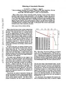
It can be observed that the pressure drops are higher than predicted by the combined Hagen-Poiseuille equation (10) and mixer KL for laminar flow for all fluids, with glycerol, the Newtonian fluid, displaying a lower increase than both Boger A and Boger B. There appears to be a further increase at high values of Re indicating a tailing off effect. This can be attributed to the viscoelasticity these fluids exhibit which predicts an additional pressure drop due to the normal stress components of the stress tensor and elastic energy storage, which is consistent with the findings of Chandra & Kale 16. Consequently, the apparent Darcy friction factors fD calculated from the pressure drop data via equation (11) are significantly higher than those predicted by the Newtonian correlation with Reynolds number. This suggests that the Boger fluids may possess much lower Reynolds numbers than those calculated for the Newtonian definition; it is postulated that this may be due to the fluid elasticity affecting the flow pattern within the mixer and therefore changing the flow regime, as previously observed in swirling viscoelastic flows22. Therefore, it is necessary to investigate the variation of pressure drop and friction factor with the generalised Reynolds number, which corrects for elastic effects through incorporation of the Weissenberg number into the viscous term.

When the measured Darcy friction factors are plotted against the generalised Reynolds number Reg as shown in Figure 5, the data approaches a single curve, albeit with a significant deviation at low values of Reg. This can be attributed to the over-prediction of the mixer wall shear rate, and thus that the vendor value of KG = 28 may be unsuitable for non-Newtonian fluids. It has been observed in stirred vessels that viscoelasticity significantly alters the flow field and therefore features local shear rates differing from those seen in a Newtonian fluid of equivalent viscosity6. Additionally, it has been reported that for various impeller designs a viscoelastic Metzner-Otto constant different in value to that used for inelastic fluids is required to fit viscoelastic data to Newtonian fluids 24; in static mixers the equivalent parameter is KG. However, at present there is no experimental measurement of local flow fields with viscoelastic fluids in a Kenics KM mixer and as such the exact value of KG is currently unknown and therefore the exact cause of this tailing effect remains unknown.

It is

speculated that the extensional viscosity may contribute to a change in the reported KG value. Grace56 described droplet break-up in the same mixer, evaluating the extensional shear rate as a function of wall shear rate and concluded that, for Newtonian immiscible systems, the extensional viscosity is a governing parameter and is approximately equal to the pipe wall shear rate. Though valid for Newtonian and inelastic fluids, it has been shown that the extensional viscosity of viscoelastic fluids is significantly greater and varies across a range of shear rates 22. Extensional viscosity data is unavailable for the Boger fluids investigated here and as such the impact of extensional shear on pressure drop and measured KG value is unknown.

Page 15 of 35

Figure 5: Pressure drop variation with generalised Reynolds number Reg; a) pressure drop ΔP, b) Darcy friction factor fD

3.2 Striation Patterns

Figure 6 displays images taken at time t = 4.84 s, i.e. 10 images after the initial image was captured.

Glycerol

Boger A

u = 0.15 m s-1

u = 0.20 m s-1

Page 16 of 35

Boger B

u = 0.30 m s-1

Figure 6: Striation patterns at mixer outlet, t = 4.84 s

It can be observed that there is a significant difference between the mixing patterns of the Newtonian glycerol and viscoelastic Boger fluids at a given superficial velocity. Primarily, the Newtonian fluid preserves the laminated striation pattern typical of a KM mixer at all velocities, whilst both Boger fluids deviate from this significantly at increasing velocities. Although evidence of this structured striation pattern exists at low velocities, as velocity increases both Boger fluids display a dual effect of both a slight “clouding” of the flow, as well as regions of greater greyscale intensity, and therefore local concentration, that do not conform to the expected Newtonian behaviour. The shape of the high intensity regions appears in two varieties: the first are spots which possess an elliptical shape close to a circular geometry, whilst the second appears in long elongated stretches as thinner single striations. The former is indicative of more solid-like behaviour in the flow persisting along the mixer length with a region of largely unmixed material not shearing into its surroundings. The latter structure is indicative of liquid-like behaviour, although the high dye concentration indicates a lack of material transfer from these striations. It is postulated that both of these deviations from Newtonian behaviour derive from the fluid elasticity, with the more elastic Boger B displaying a greater tendency towards these structures. Further, it can be noted for both viscoelastic fluids the tendency for the spot behaviour increases with increasing flow velocity, whilst the individual striation stretching occurs at lower velocities.

A further observation is that in the viscoelastic fluids there appears to be a tendency for the tracer to remain on one side of the mixer outlet, with the left hand side of the images in Figure 6 showing poorer levels of mixing than the right. This is not observed in the glycerol data, with striation patterns visible across the entire section, albeit with large regions of undyed and therefore unmixed material. This could be caused by bypassing the initial mixing element, however as the experimental set-up was not changed between different fluid passes and glycerol does not show this effect this seems extremely unlikely. It perhaps suggests that, owing to the non-circular flow cross section of the Kenics KM mixer, secondary flow systems are present. This is typical of viscoelastic fluids which possess normal stress differences, most commonly the first normal stress difference N1, as these act perpendicular to the main flow and as such set up secondary flow loops.

Page 17 of 35

It should be stated at this point that based primarily on quantitative data, it is apparent that the overall mixing quality in all cases is poor. This is to be expected as the 6-element mixer is a relatively short design, and is operating at the low end of industrial velocities. As it should be expected that the number of striations at the outlet of a KM mixer should be simply 2n, where n is the number of mixing elements, only 64 striations should be present in all cases. However, previous work has shown that velocity affects striation numbers and structure21;53. Further final mixing quality, usually a 90 % mixed confidence interval, for this mixer is defined by the reduced coefficient of variance CoVr (0.1 for the 90 % mixedness case) and is linked to mixer performance through the parameter Ki (0.87 for a Kenics KM7), indicating a mixer length to diameter ratio L/D of:

𝐶𝑜𝑉𝑟 =

𝐶𝑜𝑉 𝐶𝑜𝑉0

𝐿

= 𝐾𝑖 𝐷

(16)

𝐿 log 𝐶𝑜𝑉𝑟 = = 16.5 𝐷 log 𝐾𝑖 This would require 0.31 m of pipe, i.e. 14 mixer elements to achieve this mixing quality. However, it has previously been shown that using CoV in isolation is insufficient to fully describe mixing performance21;41;54;55, so therefore the areal analysis of the raw data must be assessed.

3.2.1

Time variation

Previous studies in laminar flow with Newtonian and non-Newtonian inelastic fluids have shown the flow to be time invariant, with local greyscale values exhibiting negligible variation from frame to frame21;53. This invariance previously allowed for a single image at an arbitrary time to be analysed to determine mixing performance. However, for both the Boger fluids studied here this is not the case. Over the image acquisition period, the striation pattern at the mixer outlet varied significantly. Further, as the superficial flow velocity increased the pattern variation also became more pronounced. Figure 7 displays the variation for Boger fluids A and B. Additionally, the statistics for both viscoelastic fluids are displayed in Figure 8.

Glycerol

Boger A

Page 18 of 35

Boger B

t=0s

t = 4.84 s

t = 9.67 s

Figure 7: Variation in striation patterns at mixer outlet over time, u = 0.2 m s-1

Glycerol

Boger A

Page 19 of 35

Boger B

Figure 8: Time variation statistics; a) area fraction, b) coefficient of variance (CoV); dotted lines indicate mean values

The time variation is most clearly seen in the CoV values. Significant variation over time can be observed, with CoV values varying by up to 20 % of the mean of all values for a given experimental condition, with Boger B possessing the greatest statistical deviation from the mean. The same variation can be observed in the 90 % mixed fraction data, with a maximum of 35 % deviation from the mean also observed. The data also shows a periodicity around a central value, indicating that a pseudo-state had indeed been attained by the point of image acquisition. Table 3 displays the averages of the 90 % mixed fractions and coefficients of variance for all conditions, with standard deviations displayed in brackets.

Table 3: Table of time-averaged image statistics Glycerol

Boger A

Boger B

Velocit

90 %

Coefficie

Calculated

90 %

Coefficie

Calculated

90 %

Coefficie

Calculated

y (m s-

mixed

nt of

mixer

mixed

nt of

mixer

mixed

nt of

mixer

1

fractio

variance

performan

fractio

variance

performan

fractio

variance

performan

n (-)

CoV (-)

ce

n (-)

CoV (-)

ce

n (-)

CoV (-)

ce

)

0.15

0.20

0.30

3.33

0.83

(±0.17)

(±0.01)

3.95

0.79

(±0.30)

(±0.02)

4.61

0.78

parameter

parameter

parameter

Ki (-)

Ki (-)

Ki (-)

0.88

3.77

0.98

(±0.00) (±0.96)

(±0.08)

0.88

4.12

1.14

(±0.00) (±0.63)

(±0.11)

0.88

4.01

0.84

Page 20 of 35

0.90

3.34

1.13

0.91

(±0.00) (±0.47)

(±0.08)

(±0.00)

3.38

1.13

0.91

(±0.00) (±0.51)

(±0.12)

(±0.00)

1.20

0.91

0.91

0.88

3.46

(±0.25)

(±0.01)

(±0.00) (±0.71)

(±0.07)

(±0.00) (±0.84)

(±0.13)

This temporal variation can only be attributed to the presence of elastic instability, due to local differences in relaxation time arising from the varied local shear rates within the mixer. Previous work discovered that for swirling flows in stirred vessels a characteristic flow map between Reynolds number Re and Weissenberg number Wi governed the shift from elastically driven flow to inertially driven22;50. The values of these parameters in this study are comparable to those indicative of unsteady flow, indicating that the flow structures observed will not be constant over time. This can only be ascribed to the generation of normal stresses which act to destabilise the inertial flow.

Owing to this temporal variation, the mean and standard deviation of the mixing quality has been assessed; averages converge to a single value using a minimum of 15 images, thus the full set of 20 images has been used to obtain averages and standard deviations for each image statistic in order to compare the data further.

3.2 Statistical Analysis 3.2.1

Areal Analysis and Coefficients of Variance

The areal distributions shown in Figure 9 display the time-averaged areal distributions, whilst Figure 10 displays coefficients of variance for all fluids at constant velocity. Please note the scale; an upper limit of 25 % has been implemented to improve clarity of the more important higher mixing fractions (> 60 %). u = 0.15 m s-1

u = 0.20 m s-1

Figure 9: Comparison of areal mixing fractions at constant fluid velocity

Page 21 of 35

u = 0.30 m s-1

(±0.00)

Figure 10: Coefficients of variance (CoV) at mixer outlet

For a given velocity, the CoV always increases from Newtonian glycerol to viscoelastic Boger fluids. However, as velocity increases CoV decreases in glycerol whilst increasing in the Boger fluids. As previously stated, the use of CoV alone may not be representative of the mixing performance of complex flow structures and therefore the areal mixing fractions must be assessed to give a more complete picture of the performance.

When the area fractions are studied, in particular the

90 % mixed fraction, it can be observed that there is a monotonic trend in the size of this fraction as elasticity increases, with a slight decrease observed from glycerol to Boger A to Boger B at all conditions. This suggests that there is a weak effect of elasticity on mixing performance, with fluid elasticity inhibiting distributive mixing processes. When the values of the other mixed fractions (except < 60 %) are observed, it can additionally be seen that as elasticity increases the area fractions each decrease. As with the 90-100 % mixed fraction, this indicates that increasing elasticity inhibits mixing performance, with a greater tendency for more solid-like regions of flow to form that do not readily mix with the surroundings.

Glycerol

Boger A

Page 22 of 35

Boger B

Figure 11: Comparison of areal mixing fractions at varying velocity

When assessing the effect of velocity on each fluid individually, it can be seen that the trends in CoV do not follow the same pattern from fluid to fluid. Whilst glycerol displays a decrease in CoV as velocity increases, Boger A displays an increase followed by a large decrease whilst Boger B displays a continual increase as velocity increases. However, the same is not true of the area fractions for each fluid. It can be observed that whilst for glycerol the fraction of the 60 % and greater mixedness levels all increase, both Boger fluids behave in a different manner. Boger A appears to show only a very slight increase in 90 % mixedness fractions as velocity increases, whilst the other fractions remain largely constant. Boger B on the other hand displays an overall decrease in the higher mixing fractions, indicating a reduction in mixing performance. This overall tendency of decreasing mixing fractions as velocity increases would appear intuitively to suggest that elasticity inhibits mixing performance. However, owing to the inverse relationship of fluid relaxation time, the key measure of elasticity in this study, and shear rate, the opposite is in fact true: as velocity increases, due to the increase in wall shear rate the fluid relaxation time decreases, indicating that the fluid would display less elastic-like behaviour at higher fluid superficial velocities. This would therefore indicate that the complex interaction of fluid elasticity and flow dynamics is causing an apparently contradictory response.

It is therefore necessary to investigate the overall mixing performance against the

dimensionless parameters that govern flow inertia and elasticity in order to numerically assess the impact of the flow-elasticity interaction.

3.2.2

Assessment of trends in experimental data with dimensionless parameters

In order to determine scaling rules and assess the governing phenomena under different process conditions, it is necessary to compare mixing data to relevant dimensionless parameters. Typically, the desired final product quality would be found using either a 90 % or 95 % confidence interval, and therefore in this case the 90 % mixing fractions shall be taken as the required areal fraction. Further, in order to compare to other studies, the coefficient of variance shall also be assessed.

Page 23 of 35

Figure 12 displays the intensity of the 90% mixed fraction and coefficients of variance plotted against specific energy input ε.

Figure 12: 90% mixed fraction and CoV versus specific energy input versus; filled symbols indicate 90% mixed fraction, empty symbols indicate CoV

It can be seen that there is no clear correlation between the specific energy input and the mixing performance measured through either the coefficient of variance or 90 % mixed fraction.

In

particular, the CoV appears to show two broad trends with a reduction in this value as energy input increases for Newtonian glycerol, indicating an improvement in final mixing quality, whilst the viscoelastic Boger fluids generally show an increase in this CoV and thus a reduction in final mixing quality. This bimodal trend is seen in the areal data also, with glycerol showing an improvement in 90 % mixed fraction as energy input increases, which is consistent with previous data for this mixer geometry21 and the traditional mixing perspective that mixing quality improves as energy input increases. However, the increase in mixing performance is much more marginal for Boger fluids, with the trend suggesting no change in final mixing quality. As with the observations of pressure drop in section 3.1, this can be attributed to the elastic storage of energy within the viscoelastic fluid, thus resulting in a lack of power dissipation contributing to mixing performance and thus no observable increase in final mixing quality across the measured range. It can therefore be concluded that using specific energy input in isolation is insufficient to predict the final mixing quality of the fluid. Thus, it is necessary to explore different parameters in order to discover an underlying controlling mixing mechanism.

Page 24 of 35

Figure 13 displays the mixing performance for all conditions against individual dimensionless numbers, assessing fluid hydrodynamics and elasticity in isolation.

Figure 13: Comparison of 90% mixed fraction and coefficient of variance; a) Reynolds number Re, b) Weissenberg number Wi; filled symbols indicate 90% mixed fraction, empty symbols indicate CoV

As previously stated, there is no clear trend in the variation of coefficient of variance when all conditions are compared to both the Reynolds and Weissenberg numbers. Further, it can be seen that the 90 % mixed fraction is fairly well correlated with Reynolds number, albeit with some outliers. The data suggest that Re only weakly affects the 90% mixed fraction as calculated values remain almost constant across the measured range with a slight increase at increasing values of Re. This is consistent with vendor guidelines, though disagrees with previous work into Newtonian fluid mixing performance, where the mixed fraction markedly increases with increasing Re. This discrepancy can be attributed to both the effect of fluid elasticity not being accounted for, the narrower range of Reynolds numbers investigated in this study and also the small number of mixing elements implemented. Both Boger fluids correlate well with Weissenberg number, with a slight decrease in 90% mixed fraction as Wi increases confirming the observation that in this mixer geometry fluid elasticity inhibits mixing performance. Owing to the inelastic nature of glycerol (i.e. Wi = 0) all values for this fluid are situated on the y-axis. Thus, the limitations of these parameters are apparent, as Re and Wi cannot adequately account for both elastic and inelastic fluids and therefore an approach which seeks to combine inelastic behaviour with elastic fluids should be taken.

Figure 14 displays the same mixing performance plotted against the dimensionless groups El and Reg which combine both elastic and hydrodynamic forces.

Page 25 of 35

Figure 14: 90% mixed fraction and coefficient of variance (CoV); a) Elasticity number El, b) Generalised Reynolds number Reg; filled symbols indicate 90% mixed fraction, empty symbols indicate CoV Though both plots do show strong positive correlations of mixing performance against the dimensionless parameters, Elasticity number El cannot predict Newtonian fluid performance as the definition of El includes the Weissenberg number Wi in its definition and as previously stated this is by definition zero for inelastic fluids. The generalised Reynolds number Reg displays a single trend upon which all fluids collapse based on the 90% mixed fraction. It clearly displays that the more elastic Boger B displays the lowest values of Reg and mixing fraction, with inelastic glycerol possessing the greatest mixing fraction of highest values of Reg. As velocity increases the generalised Reynolds number also increases, and additionally mixing performance in the 90 % mixed fraction also increases. This is in line with the results obtained for Newtonian and non-Newtonian inelastic fluids in previous studies21;53, and suggests that increasing fluid velocity increases mixing performance whilst increasing fluid elasticity inhibits mixing. However, it must be stressed that this is a weak effect as the increase in 90% mixed fraction is only 2% of the total across the measured Reg range. Both El and Reg show a monotonic trend in mixing performance as each parameter increases, indicating that the experimental data all falls within one particular elastic regime. As previously noted, these values fall within the unsteady flow regime as predicted by Stokes et al.50 for both Boger fluids, with glycerol being an “inertially” driven laminar flow governed by Re alone. Given the large time variation in the data it is expected that all experiments for the Boger fluids are in an unsteady flow regime, despite the lack of data to determine the transition values between elastic, inertial and unsteady flows. The trends observed may therefore not be valid in other flow regimes, though further experimentation with a wider range of fluid elasticities and Weissenberg numbers is required to confirm this.

The above dimensionless groups therefore lead to the conclusion that the primary variable that determines mixing quality is the generalised Reynolds number Reg. Though applicable across a wider Page 26 of 35

range of fluids than Wi or El, Reg possesses several key limitations.

Firstly, the concept was

developed for use in stirred tank systems with second-order fluids, and as such uses a very specific definition of the Weissenberg number as a result of this. To date Reg has not been implemented in systems with non-second-order fluids or in non-stirred tank systems, and as such there is no additional evidence beyond this study to confirm the applicability of Reg outside of these geometries. Additionally, a relatively small range of flow conditions were implemented in this particular study owing to equipment limitations, and as such further study is required in order to validate the application of this dimensionless number to a much wider range of process conditions. Further, as strictly Reg is merely a correction for viscoelastic power input to the process, it should only be used after other parameters have failed to fully describe the flow situation, as is the case above.

4. Conclusions

Upon investigation of the mixing performance of Newtonian and viscoelastic fluids in a Kenics KM static mixer, it has been found that viscoelasticity significantly affects the mixing performance of fluids at the outlet of a 6-element Kenics KM static mixer. This manifests as a change in striation pattern from a typical lamellar structure associated with the Kenics’ helical twist element design toward a more segregated and amorphous structure. Further, the temporal variation in striation structure when a viscoelastic fluid is processed has not been previously reported, and thus elucidates a previously unknown phenomenon that has serious implications for further downstream processing. Statistical assessment of mixing performance has shown that elasticity inhibits mixing to a small degree, with the generalised Reynolds number Reg presenting the best parameter for determining mixing performance at the outlet.

The results presented represent the first investigation into mixing performance using viscoelastic fluids. Further study should include the effect of mixer scale, i.e. the internal diameter of the pipeline containing the static mixer, and should also investigate the effect of additional mixing elements. Also, implementing higher superficial velocities within the mixer, and thus extend the study to the upper limit of the laminar flow regime, would determine the validity of these observations across the entire laminar region.

Acknowledgements

John Ramsay is funded by an EPSRC Doctoral Training Grant (EP/K502984/1) from the University of Birmingham and Johnson Matthey. Page 27 of 35

Appendix A – Derivation of Generalised Reynolds Number Reg The reasoning presented below follows the same reasoning as in Bertrand et al.24, where the concept of correcting the Reynolds number for viscoelastic effects was first introduced. For a pipe system, the relationship between wall shear stress τw and pressure drop ΔP is given by:

𝜏𝑤 =

∆𝑃 𝑟 𝐿 2

(17)

Where r is the radius. For a second-order fluid, the stress is given as: 𝜏 = 𝜇𝛾̇ + 𝜓1 𝛾̇ 2

(18)

Or, in a rearranged form:

𝜏 = 𝜇𝛾̇ (1 +

𝜓1 𝛾̇ ) 𝜇

= 𝜇𝛾̇ (1 + 2𝜆𝛾̇ ) = 𝜏𝑁𝑒𝑤𝑡𝑜𝑛𝑖𝑎𝑛 (1 + 2𝑊𝑖) = 𝜏𝑁𝑒𝑤𝑡𝑜𝑛𝑖𝑎𝑛 (1 + 𝑊𝑖′) (19)

Where Wi’ = 2Wi. This can then be substituted into equation (17), and substituting for the friction factor: 𝐿

Δ𝑃 = 2𝜌𝑢2 (𝐷) 𝑓𝐷 (1 + 𝑊𝑖′)

(20)

In laminar flow, fD = 64/Re, obtaining: 𝐿

Δ𝑃 = 128𝜌𝑢2 (𝐷)

(1+𝑊𝑖′) 𝑅𝑒

(21)

𝑅𝑒

The expression 1+𝑊𝑖′ is the generalised Reynolds number Reg, which corrects the viscous term in the Reynolds number for the additional elastic stress term. Strictly speaking Reg should only be used to correct the pressure drop in viscoelastic fluid flows, in the same way that the Metzner-Otto correlation in stirred tanks only strictly corrects the power draw for non-Newtonian fluids, and caution should be taken when used outside of this specific application. This derivation assumes that the shear rate is the

Page 28 of 35

same as for Newtonian fluid flow in a pipeline, which is typically corrected for in static mixers through the use of a factor KG.

Nomenclature

Roman letters a

Power law pre-exponential

sb+1

factor b

Power law exponent

-

C

Concentration

g L-1

D

Diameter

m

El

Elasticity number

-

fD

Darcy friction factor

-

fX

Areal mixing fraction

-

G

Greyscale

-

KG

Mixer shear rate constant

-

Ki

Mixer mixing efficiency

-

constant KL

Mixer pressure drop ratio

-

factor L

Length

m

n

Number

-

N1

First normal stress difference

Pa

P

Pressure

Pa

Q

Flow rate

m3 s-1

Re

Reynolds number

-

Reg

Generalised Reynolds number

-

t

Time

s

u

Superficial velocity

m s-1

Wi

Weissenberg number

-

X

Areal mixing intensity

-

𝛾̇

Shear rate

s-1

Δ

Difference

-

Greek letters

Page 29 of 35

ε

Specific energy input

J kg-1

η

Fluid apparent viscosity

Pa s

λ

Fluid relaxation time

s

μ

Fluid Newtonian viscosity

Pa s

ρ

Fluid density

kg m-3

σ

Variance

-

τ

Shear stress

Pa

ψ

Normal stress coefficient

Pa s-2

List of figures

Figure 1: a) Equipment set-up diagram; b) static mixer section dimensions Figure 2: a) Shear stress τ and viscosity η versus shear rate 𝛾̇ for Boger fluid; b) First normal stress differences N1 and relaxation times λ for Boger fluids Figure 3: Example PLIF calibration curve of rhodamine-6G concentration against average image greyscale value Figure 4: Pressure drop variation; a) Flow rate Q, b) Reynolds number Re, c) Darcy friction factor fD Figure 5: Pressure drop variation with generalised Reynolds number Reg; a) pressure drop ΔP, b) Darcy friction factor fD Figure 6: Striation patterns at mixer outlet, t = 4.84 s Figure 7: Variation in striation patterns at mixer outlet over time, u = 0.2 m s-1 Figure 8: Time variation statistics; a) area fraction, b) coefficient of variance (CoV); dotted lines indicate mean values Figure 9: Comparison of areal mixing fractions at constant fluid velocity Figure 10: Coefficients of variance (CoV) at mixer outlet Figure 11: Comparison of areal mixing fractions at varying velocity Figure 12: 90% mixed fraction and CoV versus specific energy input versus Figure 13: Comparison of 90% mixed fraction and coefficient of variance; a) Reynolds number Re, b) Weissenberg number Wi Figure 14: 90% mixed fraction and coefficient of variance (CoV); a) Elasticity number El, b) Generalised Reynolds number Reg

List of tables

Page 30 of 35

Table 1: Experimental conditions for PLIF experiments Table 2: Fluid compositions and rheological parameters Table 3: Table of time-averaged image statistics

Literature Cited (1) Barnes H. A Review of the Rheology of Filled Viscoelastic Systems. Rheology Reviews 2003;1-36. (2) Ihejirika I, Ein-Mozaffari F. Using CFD and ultrasonic velocimetry to study the mixing of pseudoplastic fluids with a helical ribbon impeller. Chemical Engineering & Technology 2007;30:606-614. (3) Chavan VV. Close-clearance helical impellers: A physical model for newtonian liquids at low Reynolds numbers. AIChE J 1983;29:177-186. (4) Chhabra R, Bouvier L, Delaplace G, Cuvelier G, Domenek S, Andre C. Determination of mixing times with helical ribbon impeller for non-Newtonian viscous fluids using an advanced imaging method. Chemical Engineering & Technology 2007;30:1686-1691. (5) Jahangiri M. Velocity distribution of helical ribbon impeller in mixing of polymeric liquids in the transition region. Iranian Polymer Journal 2007;16:731-739. (6) Ramsay J, Simmons MJH, Ingram A, Stitt EH. Mixing of Newtonian and viscoelastic fluids using GÇ£butterflyGÇØ impellers. Chemical Engineering Science 2016;139:125-141. (7) Paul EL, Atiemo-Obeng VA, Kresta SM. Handbook of Industrial Mixing. John Wiley & Sons, 2003. (8) Rahmani RK, Keith TG, Ayasoufi A. Numerical simulation and mixing study of pseudoplastic fluids in an industrial helical static mixer. Journal of Fluids EngineeringTransactions of the Asme 2006;128:467-480. (9) van Wageningen WFC, Kandhai D, Mudde RF, van den Akker HEA. Dynamic flow in a Kenics static mixer: An assessment of various CFD methods. AIChE J 2004;50:1684-1696. (10) Rauline D, Le Blevec JM, Bousquet J, Tanguy PA. A comparative assessment of the performance of the Kenics and SMX static mixers. Chemical Engineering Research & Design 2000;78:389-396. Page 31 of 35

(11) Avalosse T, Crochet MJ. Finite-element simulation of mixing .2. Three-dimensional flow through a kenics mixer. AIChE J 1997;43:588-597. (12) Regner M, Ostergren K, Tragardh C. Effects of geometry and flow rate on secondary flow and the mixing process in static mixers - A numerical study. Chemical Engineering Science 2006;61:6133-6141. (13) Saatdjian E, Rodrigo AJS, Mota JPB. On chaotic advection in a static mixer. Chemical Engineering Journal 2012;187:289-298. (14) Hobbs DM, Muzzio FJ. Optimization of a static mixer using dynamical systems techniques. Chemical Engineering Science 1998;53:3199-3213. (15) Shah NF, Kale DD. Pressure-Drop for Laminar-Flow of Non-Newtonian Fluids in Static Mixers. Chemical Engineering Science 1991;46:2159-2161. (16) Chandra KG, Kale DD. Pressure-Drop for Laminar-Flow of Viscoelastic Fluids in Static Mixers. Chemical Engineering Science 1992;47:2097-2100. (17) Li HZ, Fasol C, Choplin L. Pressure drop of Newtonian and non-Newtonian fluids across a Sulzer SMX static mixer. Chemical Engineering Research & Design 1997;75:792-796. (18) Kumar G, Upadhyay SN. Pressure drop and mixing behaviour of non-Newtonian fluids in a static mixing unit. Canadian Journal of Chemical Engineering 2008;86:684-692. (19) Laporte M, Loisel C, Della Valle D, Riaublanc A, Montillet A. Flow process conditions to control the void fraction of food foams in static mixers. Journal of Food Engineering 2014;128:119-126. (20) Thakur RK, Vial C, Nigam KDP, Nauman EB, Djelveh G. Static mixers in the process industries - A review. Chemical Engineering Research & Design 2003;81:787-826. (21) Alberini F, Simmons MJH, Ingram A, Stitt EH. Use of an areal distribution of mixing intensity to describe blending of non-Newtonian fluids using PLIF. AIChE J 2013;60:332342. (22) Stokes JR. Swirling Flow of Viscoelastic Fluids [ University of Melbourne; 1998. (23) Ozcantaskin NG, Nienow AW. Mixing Viscoelastic Fluids with Axial-Flow Impellers - FlowFields and Power-Consumption. Food and Bioproducts Processing 1995;73:49-56.

Page 32 of 35

(24) Bertrand F, Carreau P, La Fuente EB-D, Tanguy PA. Mixing Of Viscoelastic Fluids. Engineering and Food for the 21st Century. CRC Press; 2002. (25) Faes M, Glasmacher B. Measurements of micro- and macromixing in liquid mixtures of reacting components using two-colour laser induced fluorescence. Chemical Engineering Science 2008;63:4649-4655. (26) Hall JF, Barigou M, Simmons MJH, Stitt EH. Comparative study of different mixing strategies in small high throughput experimentation reactors. Chemical Engineering Science 2005;60:2355-2368. (27) Szalai ES, Arratia P, Johnson K, Muzzio FJ. Mixing analysis in a tank stirred with Ekato Intermig((R)) impellers. Chemical Engineering Science 2004;59:3793-3805. (28) Zalc JM, Alvarez MM, Muzzio FJ, Arik BE. Extensive validation of computed laminar flow in a stirred tank with three Rushton turbines. AIChE J 2001;47:2144-2154. (29) Pianko-Oprych P, Nienow AW, Barigou M. Positron emission particle tracking (PEPT) compared to particle image velocimetry (PIV) for studying the flow generated by a pitchedblade turbine in single phase and multi-phase systems. Chemical Engineering Science 2009;64:4955-4968. (30) Gabriele A, Nienow AW, Simmons MJH. Use of angle resolved PIV to estimate local specific energy dissipation rates for up- and down-pumping pitched blade agitators in a stirred tank. Chemical Engineering Science 2009;64:126-143. (31) Stobiac V, Fradette L, Tanguy PA, Bertrand F. Pumping Characterisation of the Maxblend Impeller for Newtonian and Strongly Non-Newtonian Fluids. Canadian Journal of Chemical Engineering 2014;92:729-741. (32) Kling K, Mewes D. Two-colour laser induced fluorescence for the quantification of microand macromixing in stirred vessels. Chemical Engineering Science 2004;59:1523-1528. (33) Arratia PE, Muzzio FJ. Planar laser-induced fluorescence method for analysis of mixing in Laminar flows. Industrial & Engineering Chemistry Research 2004;43:6557-6568. (34) Alvarez MM, Zalc JM, Shinbrot T, Arratia PE, Muzzio FJ. Mechanisms of mixing and creation of structure in laminar stirred tanks. AIChE J 2002;48:2135-2148.

Page 33 of 35

(35) Chung KHK, Simmons MJH, Barigou M. Angle-Resolved Particle Image Velocimetry Measurements of Flow and Turbulence Fields in Small-Scale Stirred Vessels of Different Mixer Configurations. Industrial & Engineering Chemistry Research 2009;48:1008-1018. (36) Guillard F, Tragardh C, Fuchs L. A study on the instability of coherent mixing structures in a continuously stirred tank. Chemical Engineering Science 2000;55:5657-5670. (37) Shervin CR, Raughley DA, Romaszewski RA. Flow Visualization Scaleup Studies for the Mixing of Viscoelastic Fluids. Chemical Engineering Science 1991;46:2867-2873. (38) Fradette L, Thome G, Tanguy P, Takenaka K. Power and mixing time study involving a Maxblend (R) impeller with viscous Newtonian and non-Newtonian fluids. Chemical Engineering Research & Design 2007;85:1514-1523. (39) Rafiee M, Bakalisa S, Fryer PJ, Ingram A. Study of laminar mixing in kenics static mixer by using Positron Emission Particle Tracking (PEPT). Procedia Food Science 2011;1:678-684. (40) Mihailova O, Lim V, McCarthy MJ, McCarthy KL, Bakalis S. Laminar mixing in a SMX static mixer evaluated by positron emission particle tracking (PEPT) and magnetic resonance imaging (MRI). Chemical Engineering Science 2015;137:1014-1023. (41) Kukukova A, Aubin J, Kresta SM. A new definition of mixing and segregation: Three dimensions of a key process variable. Chemical Engineering Research & Design 2009;87:633-647. (42) Danckwerts PV. The Effect of Incomplete Mixing on Homogeneous Reactions. Chemical Engineering Science 1958;8:93-102. (43) Stamatopoulos K, Batchelor HK, Alberini F, Ramsay J, Simmons MJH. Understanding the impact of media viscosity on dissolution of a highly water soluble drug within a USP 2 mini vessel dissolution apparatus using an optical planar induced fluorescence (PLIF) method. International Journal of Pharmaceutics 2015;495:362-373. (44) Fontaine A, Guntzburger Y, Bertrand F, Fradette L, Heuzey MC. Experimental investigation of the flow dynamics of rheologically complex fluids in a Maxblend impeller system using PIV. Chemical Engineering Research and Design 2013;91:7-17. (45) Seyssiecq I, Tolofoudye A, Desplanches H, Gaston-Bonhomme Y. Viscoelastic liquids in stirred vessels - Part I: Power consumption in unaerated vessels. Chemical Engineering & Technology 2003;26:1155-1165.

Page 34 of 35

(46) Boger DV, Yeow YL. The Impact of Ideal Elastic Liquids in the Development of NonNewtonian Fluid-Mechanics. Experimental Thermal and Fluid Science 1992;5:633-640. (47) Mackay ME, Boger DV. An Explanation of the Rheological Properties of Boger Fluids. Journal of Non-Newtonian Fluid Mechanics 1987;22:235-243. (48) James DF, Yip R, Currie IG. Slow flow of Boger fluids through model fibrous porous media. Journal of Rheology 2012;56:1249-1277. (49) Magda JJ, Lou J, Baek SG, Devries KL. 2Nd Normal Stress Difference of A Boger Fluid. Polymer 1991;32:2000-2009. (50) Stokes JR, Graham LJW, Lawson NJ, Boger DV. Swirling flow of viscoelastic fluids. Part 2. Elastic effects. Journal of Fluid Mechanics 2001;429:117-153. (51) Stokes JR, Boger DV. Mixing of viscous polymer liquids. Physics of Fluids 2000;12:14111416. (52) Barnes HA. A Handbook of Elementary Rheology. University of Wales, Institute of NonNewtonian Fluid Mechanics, 2000. (53) Alberini F, Simmons MJH, Ingram A, Stitt EH. Assessment of different methods of analysis to characterise the mixing of shear-thinning fluids in a Kenics KM static mixer using PLIF. Chemical Engineering Science 2014;112:152-169. (54) Kukukova A, Noel B, Kresta SM, Aubin J. Impact of Sampling Method and Scale on the Measurement of Mixing and the Coefficient of Variance. AIChE J 2008;54:3068-3083. (55) Kukukova A, Aubin J, Kresta SM. Measuring the Scale of Segregation in Mixing Data. Canadian Journal of Chemical Engineering 2011;89:1122-1138.

(56) Grace, H.P. Dispersion phenomena in high viscosity immiscible fluid systems and application of static mixers as dispersion devices in such systems. Chemical Engineering Communications 1982;14:225-277.

Page 35 of 35