Nov 6, 2009 - reduce the gap between simulation and real-world perfor- mance. .... inter-packet interval of 16ms on channel 26 for durations of. 1, 6 and 12 ...
M&M: Multi-level Markov Model for Wireless Link Simulations ´ Carreira-Perpin˜ an ´ and Alberto E. Cerpa Ankur Kamthe, Miguel A. Electrical Engineering and Computer Science University of California - Merced
{akamthe,mcarreira-perpinan,acerpa}@ucmerced.edu
Abstract
General Terms
802.15.4 links experience different level of dynamics at short and long time scales. This makes the design of a suitable model that combines the different dynamics at different timescales a non-trivial problem. In this paper, we propose a novel multilevel approach involving Hidden Markov Models (HMMs) and Mixtures of Multivariate Bernoullis (MMBs) for modeling the long and short time scale behavior of wireless links using experimental data traces collected from multiple 802.15.4 testbeds. We characterize the synthetic traces generated from the model of the wireless link in terms of statistical characteristics as compared to an empirical trace with similar PRR characteristics, such as the mean and variance of the packet reception rates from the data traces, comparison of distributions of run lengths and conditional packet delivery functions of successive packet receptions (1’s) and losses (0’s). We modified TOSSIM to utilize data traces created using our modeling approach and compare them against the existing radio model in TOSSIM, which uses the Closestfit Pattern Matching model for modeling variations in noise which affect the link quality. The results show that our proposed modeling approach is able to mimic the behavior of the data traces quite closely, with difference in packet reception rates of the empirical and simulated traces of less than 2.5% on average and 9% in the worst case. Moreover, the simulated links from our proposed approach were able to account for long runs of 1’s and 0’s as observed in empirical data traces.
Algorithm, Measurement, Performance, Design, Experimentation
Categories and Subject Descriptors I.6.5 [Simulation and Modeling]: Model Development—Modeling methodologies; C.2.1 [ComputerCommunication Networks]: Network Architecture and design—Wireless communication
Permission to make digital or hard copies of all or part of this work for personal or classroom use is granted without fee provided that copies are not made or distributed for profit or commercial advantage and that copies bear this notice and the full citation on the first page. To copy otherwise, to republish, to post on servers or to redistribute to lists, requires prior specific permission and/or a fee. SenSys’09, November 4–6, 2009, Berkeley, CA, USA. Copyright 2009 ACM 978-1-60558-748-6 ...$5.00
Keywords Simulation, 802.15.4 Low Power Wireless Networks, Wireless Channel Model, Hidden Markov Models, Mixture of Multivariate Bernoulli
1
Introduction
The common denominator in all wireless sensor networks (WSNs), regardless of their underlying application, is the use of the radio to communicate information extracted from the sensed environment and, more importantly, to coordinate with other nodes. Consequently, radio communication and intelligent usage of the radio is a critical component of wireless distributed system in general and WSNs in particular. Due to the low power nature of WSNs, the radio used for communication is especially susceptible to changes in the quality of the wireless medium resulting in packet losses which can be attributed to limited transmission power levels as well as multipath effects resulting from lack of frequency diversity. Experiments [28] conducted with these low-power radio equipped sensor nodes have shown, using empirical measurements, that there exists a “gray area” within the communication range of sensor radios where the packet reception varies widely. Data collected using SCALE [4], led to the following conclusions: (i) no clear correlation between packet delivery and distance in an area of more than 50% of the communication range, (ii) temporal variations of packet delivery are correlated with mean reception rate of each link, and (iii) percentage of asymmetric links in a sensor network varies from 5% to 30%. These studies [28, 4, 5, 6, 25] help confirm that low power wireless communication is unpredictable, is sensitive to changes in the environment and is known to significantly change over different time scales. In systems research, a well-designed simulator provides users with the ability to test new ideas in an inexpensive manner. The simulator models the key elements of a given system, for example: hardware such as the CPU, network interfaces, sensors, etc. and software such as the operating system. This allows the user to focus his attention on the design, testing and analysis of algorithms in a controlled and repeatable environment. Recent studies [21, 15] have indicated the presence of a wide chasm between the real world radio channel behavior and existing radio channel models in
wireless simulators. This leads to significant differences in performance of a system in simulation as compared to a real world deployment. Thus, improving wireless simulators by incorporating accurate and robust radio channel models will reduce the gap between simulation and real-world performance. To reach this goal, we believe it is required to collect data traces of packet reception information over long periods of time at fine granularity. This data would be the seed for creating radio channel models that would help simulate more realistic packet losses, thus helping application designers increase the robustness of their applications by accounting in simulation for losses in the wireless medium. In this paper, we propose a novel multilevel approach involving Hidden Markov Models (HMMs) and Mixtures of Multivariate Bernoullis (MMBs) for modeling the long and short time scale behavior of links in wireless sensor networks, that is, the binary sequence or trace of packet receptions (1s) and losses (0s) in the link. In this approach, a HMM models the long-term evolution of the trace (level 1) as transitions among a set of unobserved, level-1 states. These states typically correspond to a roughly constant packet reception rate (as determined by the data) and might correspond to different regimes of the link. Within each level-1 state, the short-term evolution of the trace (level 2) is modeled by either another HMM or by a MMB. This captures the faster, but not random, variations of the sequence of packet receptions and losses. We characterize the synthetic traces generated from the model in terms of several statistical measures: moments (mean and variance) of the distribution of packet reception traces, run length distributions of packet receptions and of packet losses, and conditional packet delivery functions (CPDFs). To compare run length and CPDF distributions, we designed a new metric called the NearestNeighbor Distance. This metric aims to solve the problem of comparing distributions with unequal supports. In addition, a full implementation of the M&M model for the TOSSIM simulator is provided. The rest of the paper is organized as follows: A review of related work for modeling the behavior of wireless links is provided in Section 2. In Section 3, we identify issues that need to be addressed to resolve the deficiencies in link models for WSN simulators and propose a new Markov-based modeling approach for addressing these issues. Section 4 contrasts the modeling of links in existing WSN simulators against our proposed approach. Finally, in Section 5, we discuss issues related to our modeling approach and in Section 6 summarize the results and discuss future work.
2
Background and Related Work
Models for characterizing the behavior of wireless links have been a widely studied area in networking literature [22]. These studies can be classified into radio propagation models and packet loss models. Radio propagation models predict the average received signal strength and its variability at a given distance from the transmitter. In contrast, packet loss models try to discover the underlying bursty packet loss distribution. Errors in packet reception can be attributed to causes such as interference in the channel and fading effects which lead to irrecoverable bit errors. The Gilbert
model [10] is a probabilistic model for simulating burst noise in data transmission channels. In this model, a Hidden Markov model with two states is used to generate noise bursts, the first state has zero probability of encountering an error whereas the other state has a certain fixed non-zero probability for transmission errors. Analysis of traces [20] for the AT&T Wavelan system concluded that loss behavior could not be accounted by the 2-state Markov model. They proposed a methodology to model the error-free and error traces using exponential and Pareto distributions to model segments of the trace. Traces modeled [26] from measurements of Internet packet loss compared between a Bernoulli model, 2-state Markov chain model and kth order Markov chains to check for the accuracy of the loss estimation over 38 stationary trace segments. They concluded that all these models are inadequate as they could not accurately model losses in their dataset.
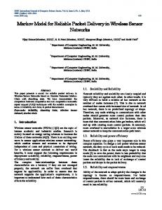
Figure 1. SE testbed: 25 groups of three nodes each separated by a distance of 40cm. Nodes are placed at fixed locations along the corridor ceiling of the building. Markov-Based Trace Analysis (MTA) [13] and Multiple MTA [14] approaches propose modeling channel errors by decomposing a trace with non-stationary properties into a set of piecewise stationary traces consisting of “lossy” and “error free” states. Lossy states exhibit stationarity, where a sequence of lossy states can be modeled by a traditional discrete time Markov chain (DTMC). In [24], HMMs were proposed for modeling packet reception traces and choosing a model based on the likelihood criterion. Markov-based stochastic chains were proposed [12] to model 802.11b channel behavior for bit errors and packet losses. The study compared the performance of high order Markov chains, 2-state Hidden Markov Models and hierarchical Markov Models and concluded that Markov chains of order 9 (i.e., 29 states) are required for accurate models for the bit error process. These studies helped reinforce the notion that for any modeling approach to simulate behavior of wireless links, the model needs to account for the long and short term variations in the link quality. Also, the model should be easy to train and show close correlation between the input and the simulated data traces.
Testbed Program Num. Expts. Duration Num. Packets/Expt. CC2420 Tx power levels SE RssiDemo 9 1 hour 230400 1-31 SE RssiDemo 1 6 hours 1382400 7 SE RssiDemo 3 12 hours 2764800 8,9,11 SE RssiSample 3 30 minutes 196608 MoteLab RssiDemo 18 30 minutes 115200 31 MoteLab RssiSample 3 30 minutes 196608 Table 1. Summary of experiments conducted on the MoteLab and SE testbeds (Note: 802.15.4 channel 26 is used in all experiments).
exp24
exp26
exp28
Avg. Network Throughput (Kbps)
9 8.8 8.6
3 Wireless Link Modeling 3.1 Collection of Packet Reception Traces
8.4 8.2 8 7.8 7.6 20:00
00:00
04:00
08:00 Hour of Day
12:00
16:00
Figure 2. Variation of the average data throughput per hour for all good and intermediate links in the network.
2.1
resentative model of a real environment. In contrast, in this paper, we propose the modeling of correlations between successive packet receptions and failures from a given packet reception trace as the packet reception traces are a direct indicator of the link quality.
TOSSIM
TOSSIM [17] is a discrete event simulator for sensor networks running on the TinyOS operating system. It allows users to write TinyOS code in a simulation environment that is scalable and bridges the gap between algorithm testing and application development. TOSSIM simulates behavior of the CPUs, radios and sensors in different sensor nodes, networking stacks and other OS primitives. TOSSIM supports several radio models, namely the Simple Propagation model, the Link Layer model [29] and the CPM model [16]. In the Simple Propagation model, every node can receive packets transmitted by any other node. The Link Layer model specifies the behavior of the wireless link depending on the radio and the channel characteristics for static and low-dynamic environments. CPM is based on a statistical model created from noise reading traces collected from the deployment environment. It computes the probability distribution of nt given the noise readings (nt−k , nt−k+1 , ...nt−1 ), where k is the duration of noise history considered by the model. A k = 0 would make each noise value independent, while k equal to the length of the trace would provide an exact replay of the noise trace. In a recent paper [23], two approaches (Expected Value PMF and Average Signal Power Value) were proposed to estimate the signal power of missing packets in a packet reception trace, and, using this data the CPM algorithm models the variations in packet signal strength. These existing models require the modeling of two separate physical layer measurements, namely, RSSI and noise/interference values to create a rep-
In order to create an accurate packet loss model, we required a comprehensive database of packet reception traces of links having different reception rates. For this task, we collected data from a 75 node MoteIV Tmote Sky testbed deployed along the ceiling of the Science and Engineering Building (SE testbed). Each mote is comprised of an ultra low power Texas Instruments MSP430 F1611 microcontroller featuring 10KB of RAM, 48KB of flash and a 802.15.4 compliant Chipcon CC2420 radio (channel 26) for wireless communication. The node locations are fixed for the duration of our experiments (refer Figure 1 for details). All the motes in a group are connected to a Linksys NSLU2 network storage device via an USB hub. The Linksys NSLU2 device is used to bridge serial communication between the motes and a central server over the local network. We performed a number of experiments to collect packet reception traces from a diverse set of links (see Table 1). In each experiment, we have one fixed sender and multiple receivers. The sender sends 64 packets per second with an inter-packet interval of 16ms on channel 26 for durations of 1, 6 and 12 hours. The receivers record the sequence number, received signal strength (RSSI) and link quality indicator (LQI) values of each received packet. We also collected the same data from the Motelab testbed [27] but the duration of each experiment was limited to 30 minutes due to storage concerns regarding the large amount of data generated in every run. After each experiment, we created records or traces of packet reception for each of the receiver nodes. In addition, we also gathered noise data (channel 26) for all nodes using the RssiSample program on both the testbeds. The length of the noise traces is equivalent to the meyer − heavy trace collected in [16]. The noise traces are meant to be utilized for a faithful comparison between the TOSSIM simulation model and our proposed approach.
3.2
Exploratory Data Analysis
In this section, we highlight issues that need to be addressed when modeling 802.15.4 wireless links. We term links having packet reception rate (PRR) < 10% as bad or poor links, links having PRR between 10% and 90% as intermediate links and links having PRR greater than 90% as
1
0.8
0.8
0.8
0.6 0.4 0.2 0
PRR (mean = 0.19)
1
PRR (mean = 0.65)
PRR (mean = 0.42)
1
0.6 0.4 0.2
0
10
20 30 40 time (in minutes)
50
0
60
0.4 0.2
0
(a) Link1-Hour1, PRR=42%
10
20 30 40 time (in minutes)
50
0
60
0
(b) Link1-Hour2, PRR=65% −84
−86
−86
−86
−88
−88
−88
−92 −94 −96
RSSI (dBm)
−84
−90
−90 −92 −94
0
10
20 30 40 time (in minutes)
50
(d) Link1-Hour1, PRR=42%
60
−96
10
20 30 40 time (in minutes)
50
60
(c) Link1-Hour3, PRR=19%
−84
RSSI (dBm)
RSSI (dBm)
0.6
−90 −92 −94
0
10
20 30 40 time (in minutes)
50
(e) Link1-Hour2, PRR=65%
60
−96
0
10
20 30 40 time (in minutes)
50
60
(f) Link1-Hour3, PRR=19%
Figure 3. Variation in PRR and RSSI by hour for a typical intermediate quality link. Figure shows that PRR and RSSI values are stable for short periods of time. Exp. CC2420 Good Bad Interm Inactive # Tx. Lvl. 24 11 20(48%) 8(19%) 7(17%) 7(16%) 26 10 19(45%) 7(17%) 3(7%) 13(31%) 28 8 19(45%) 10(24%) 3(7%) 10(23%) Table 2. Summary of variation of link quality in a network as a function of sender radio transmission power.
good links. Links having PRR = 0% are termed as inactive links. Prior studies have shown that 802.15.4 links can vary significantly over time [4, 6, 18]. In Figure 2, the average network throughput per hour averaged over all the links having PRR > 10% in the network is shown as a function of time of day for the 12 hour experiments. The figure clearly shows that the average network throughput is not constant, but fluctuates with time. This is a clear indication of variation of PRR across nodes in the network. The radio transmission power levels in experiments 24, 26 and 28, correspond to values 11, 10 and 8 in the CC2420 registers. This would lead one to think that, the throughput should be highest for experiment 24, followed by level 26 and 28, respectively. However, from the data, we see that the throughput for experiment 24 is less than that of the others. This can be explained by the higher total number of intermediate links (see Table 2) compared to the other experiments. An interesting artifact of the environment can be see in Figure 2, which shows a fairly
consistent decrease in throughput from midnight to midday in all three experiments. From our experimental data, we observed that good and bad links are relatively stable over time whereas intermediate links show significant variation in link quality over time. This is consistent with previous findings reported in [4, 6]. In general, in simulation, it is easy to model good links as they do not show significant variation with time [19, 23]. On the other hand, there is a significant difference between the models of intermediate links in simulation and the real-world. If the accuracy of simulation models of these intermediate links were improved, then it is possible that WSN application simulations could show the potential benefits of using these intermediate links when their quality is high enough for transporting data instead of permanently ignoring or blacklisting them. In addition, it would help application designers to test performance of algorithms for the common case, and the corner cases that are one of the causes of protocol failure. To emphasize this point, we plot the variation in PRR and RSSI of a representative intermediate link. For this link (see Figure 3), the PRR is plotted as a function of time, where each PRR value is calculated for a two second interval (i.e., for 128 consecutive packets at a time). Figure 3 also shows the corresponding variation in RSSI values of the received packets. From Figure 3, we see that the average PRR of link 1 is 42%, 65% and 19% for hours 1, 2 and 3, respectively and the corresponding average RSSI values are -91.85 dBm, -91.8 dBm and -91.67 dBm, respectively. In each hour, we
00011111 10001110 00011111 00011110
p(x1 |q1 )
p(x0 |q0 )
q0
p(q1 |q0 )
q1
p(q2 |q1 )
q2
...
x3
x2 p(x2 |q2 )
x1
p(x3 |q3 )
x0
...
p(q3 |q2 )
q3
p(q4 |q3 )
...
t =0 t =1 t =2 t =3 Figure 4. Graphical model of a HMM which emits binary strings xt of length 8. In the M&M model, this is the L1– HMM, and p(xt |qt ) is itself a HMM or a MMB. see that the PRR and RSSI values fluctuates widely, cycling between good, intermediate and bad states. In each state, the link is relatively stable for a given period of time before a significant change in link quality. A closer look at the sequence of received packets within few tens of seconds reveals that packet receptions and losses are not independent i.e., intermediate links show significant bursty behavior. This shows that links of intermediate quality manifest highly dynamic behavior over time at different time scales, thus highlighting the non-trivial nature of the modeling problem for such links.
3.3
Our Modeling Approach
We consider our observed data as binary sequences where 1 indicates successful packet reception and 0 indicates lost or corrupted packets. (We will also consider a sequence of continuous values, namely the reception rates in [0, 1] indicating the average over a binary window.) The fundamental motivation for our modeling approach is that observed traces display structure at different temporal scales. In Figure 5(a), for example, one can see that over a period of minutes the link seems to switch between two states: one with PRR ≈ 0.6 and the other with PRR ≈ 0.8. We call this the long-term dynamics. In a period of seconds, however, while the PRR may stay roughly constant at 0.6, it is more likely to observe a bursty sequence 0000111111 than a wildly oscillating sequence 1010101101. We call this the short-term dynamics. In order to simulate realistically the behavior of links, we want a model that is flexible enough to replicate this multiscale structure, and we want to estimate its parameters (which determine its typical PRRs or its local burstiness) from observed traces. We now describe the details of our model, the Multi-level Markov (M&M) model; appendices A–B give an overview of hidden Markov models and mixtures of multivariate Bernoulli distributions.
3.4
The Multi-level Markov (M&M) Model
We model a possibly infinite binary sequence (the data trace) as a sequence of binary strings (windows) xt of length W , as shown in Figure 4. A level-1 hidden Markov model (L1–HMM) with Q1 different states q = 1, . . . , Q1 models transitions between long-term states, and has Q21 tunable parameters ai j (the transition probabilities p(q = j|q = i)). Each long-term state q has its own distribution p(x|q) of emitting binary W -windows, which captures the short-term behavior of the link in that state—that is, the dynamics of the
Original PRR
Simulated PRR Simulated PRR by L2–HMM by L2–MMB Mean±StdDev Mean±StdDev 0.31 0.34 ± 0.004 0.31 ± 0.010 0.59 0.61 ± 0.006 0.56 ± 0.005 0.61 0.62 ± 0.002 0.62 ± 0.002 0.62 0.59 ± 0.004 0.61 ± 0.006 0.71 0.68 ± 0.010 0.69 ± 0.002 0.72 0.70 ± 0.019 0.71 ± 0.007 Table 3. Summary Statistics of Links: Comparison between the original trace and simulated traces from the M&M model using HMMs and MMB, respectively. Both the L2 modeling approaches work well for simulating the behavior of the traces. variations in consecutive packet reception successes or failures that has its own parameters (described below). Thus, W controls the tradeoff of short vs. long term. In this paper, we studied two types of short-term, or level-2, models p(x|q): • A hidden Markov model (L2–HMM). This has (1) a set of Q2 short-term states (different from those of the L1– HMM) and its own Q22 transition probabilities, and (2) a (univariate) Bernoulli emission distribution with parameter p. Thus, this is a sequential model: to emit a W -window we sample W times from the L2–HMM. Note that the L2–HMM for long-term state i has its own parameters, different from those of the L2–HMM for a different long-term state j. • A mixture of multivariate Bernoulli distributions (L2– MMB). This mixture has M components, and each component has W + 1 parameters: a mixture proportion and a vector p = (p1 , . . . , pW ) of Bernoulli parameters. Thus, this is not a sequential model: to emit a W -window we pick a component at random (according to their proportions) and then we sample from its W dimensional Bernoulli the W -window at once. We report experimental results with both models below. In both models, using a sufficiently large number of short-term states Q2 or mixture components M allows us to model arbitrarily complex distributions of W -dimensional binary windows; for example, more or less bursty sequences. Importantly, note that if we modeled p(x|q) as a single Bernoulli (i.e., M = 1), then bits within the window would be independent from each other, leading to unrealistically oscillating behavior. The average PRR of a long-term state i is the mean of its emission distribution p(x|q = i). Next, we explain how to simulate a binary trace from our model (sampling), and how to estimate good model parameters from measured data (learning).
3.4.1
Sampling
In order to generate a trace of length L bits from the model, we sample as follows: 1. Generate a long-term state sequence of length L/W using the transition probabilities of the L1–HMM. 2. For each long-term state q of this sequence, we sample a W -window x from its p(x|q) (i.e., the corresponding
5
0.9 0.8
0.6
4
10
3
10
2
10
1
10
0
10
0
0.5
20 40 60 Run Length of 1s
80
5
111110011011111111111010001 001111100110011110110101111 011010100101111001110111000 111111100011111101100001111 11111101011100111110...........
0.3 0.2 0.1 0 0
15
30 time (in minutes)
45
60
10
Conditional Probability
0.4
Weighted Occurrences
PRR (mean = 0.72)
0.7
10
Conditional Probability
Weighted Occurrences
1
4
10
3
10
2
10
1
10
0
10
0
50 100 Run Length of 0s
150
1 0.8 0.6 0.4 0.2 0 0
20 40 Run Length of 1s
73
1 0.8 0.6 0.4 0.2 0 0
112 Run Length of 0s
(a) Original PRR=72% 5
0.9 0.8
0.6
4
10
3
10
2
10
1
10
0
10
0
0.5
20 40 60 Run Length of 1s
80
5
0.3 0.2 0.1 0 0
15
30 time (in minutes)
45
60
10
Conditional Probability
111110111111111111011111001 011111101111111111111111111 111111111111110111011111110 000011111110110111000111111 01010011111111111111...........
0.4
Weighted Occurrences
PRR (mean = 0.73)
0.7
10
Conditional Probability
Weighted Occurrences
1
4
10
3
10
2
10
1
10
0
10
0
50 100 Run Length of 0s
150
1 0.8 0.6 0.4 0.2 0 0
20 40 56 Run Length of 1s
1 0.8 0.6 0.4 0.2 0 0
23 Run Length of 0s
(b) M&M L2–HMM: PRR = 73%, Q1 =6, Q2 =2 5
0.9 0.8
0.6
4
10
3
10
2
10
1
10
0
10
0
0.5
20 40 60 Run Length of 1s
80
5
0.3 0.2
111010110101111011011001110 111111110111011111011111011 111111011011001101111101110 111111010111110110111111101 11111101011100110011...........
0.1 0 0
15
30 time (in minutes)
45
60
10
Conditional Probability
0.4
Weighted Occurrences
PRR (mean = 0.76)
0.7
10
Conditional Probability
Weighted Occurrences
1
4
10
3
10
2
10
1
10
0
10
0
50 100 Run Length of 0s
150
1 0.8 0.6 0.4 0.2 0 0
20 40 62 Run Length of 1s
1 0.8 0.6 0.4 0.2 0 0
101 Run Length of 0s
(c) M&M L2–MMB: PRR = 76%, Q1 =6, M=20 Figure 5. Average PRR over time from (a) experimental 1-hour data trace, (b) simulated trace using L2–HMM and (c) simulated trace using L2–MMB, respectively. On the right side we see the statistics for each link for the weighted run lengths (WRLs) and CPDFs. Note: (i) WRL values do exist for each integer and are zero if not shown; (ii) CPDF values do not exist beyond a maximum run length, so CPDF plots are truncated at maximum run length.
L2–HMM or L2–MMB). The trace is the concatenation of the L/W windows.
3.4.2
Learning
In a machine learning approach, estimating the parameters of a probabilistic model is usually done by maximizing the log-likelihood of a given data set (one or more observed traces) over all the model parameters (transition probabilities for all short- and long-term states, mixing proportions, Bernoulli parameters). For our multilevel HMM this can be quite complex and time-consuming, so in this paper we follow a simpler learning algorithm that is slightly suboptimal but faster and relatively robust to local optima, by first estimating the L1–HMM transition probabilities, and then estimating the L2–HMM transition probabilities or the L2– MMB parameters. The training process is as follows: 1. Training the L1–HMM transition probabilities. The binary input trace is transformed into a sequence of PRRs (in [0, 1]) computed over a window size W . We define a continuous HMM with Q1 states and beta emission distributions and use the EM algorithm to estimate by maximum likelihood its beta parameters (which we then discard) and its transition probabilities, given the sequence of PRRs. We obtain good initial values for the beta parameters by running k–means on the PRR sequence. 2. Clustering the W -windows. After learning the parameters of the L1–HMM, we used the Viterbi algorithm [9] to obtain the most likely state sequence for each input trace, and grouped into the same cluster all windows assigned to the same state. Practically speaking, this tends to group windows associated with similar PRR values. 3. For each long-term state, we trained its L2–HMM or L2–MMB model only on its corresponding cluster: • L2–HMM: we used again the EM algorithm for HMMs (now having univariate Bernoulli emission distributions), resulting in the L2–HMM transition probabilities and the Bernoulli parameters for each of the Q2 short-term states. • L2–MMB: we used an EM algorithm for MMBs as described in [3], resulting in the proportion and Bernoulli W -dimensional vector for each of the M mixture components.
3.4.3
Reasons for a Multi-level Model
Instead of a multi-level approach like the M&M model, it is possible to model packet traces using just a L1–model having continuous emission distributions, which represent PRR computed over a window W , to capture the long term dynamics and the short term dynamics using the PRR value from the L1 emission distribution as the Bernoulli parameter for each of the W values in the window. This model is equivalent to the M&M model, wherein (i) for the L2–HMM, Bernoulli emission probability values for both states is c, and (ii) for the L2–MMB, M = 1 and the vector of Bernoulli parameters of length W is p = c×(1, . . . , 1) where c is the PRR outputted by the emission distribution of the L1–model. The model would only capture the long-term PRR dynamics. However, in a pure L1–model, we can see that the short-term correlations are not captured correctly because each value in the
W -length window is now independent and hence, uncorrelated to its neighbors. When training, the duration of our longest data traces was 12 hours. The level of long-term dynamics for traces up to 12 hours can be accounted for using the M&M model. For longer duration traces, of the order of days, months, year, the level of long-term dynamics might be greater than that of the 12 hour traces. For modeling such traces, a 2-level model may not suffice. However, the current modeling approach can be easily extended to longer timescales using a N-level hierarchy.
3.5
Evaluation of the M&M model
To evaluate the performance of our approach, we trained models for links with different reception rates from the experimental data traces (training set, length = 230400). As the problem is unsupervised (there is no ground truth to compare with) and the generated sequences can have any length, we do not compare the likelihood value that the models produce for a trace. Instead, we compare on the basis of statistics computed on the traces versus a different set of unseen data traces (testing set) having similar PRR characteristics. For each link, we proceeded as follows: (1) We learned the model parameters given the (training set) data traces; we tried both versions (L2–HMM and L2–MMB), different window lengths W (though most of our results are for W = 128), and different values of Q1 , Q2 and M (model size). (2) For each model, we sampled a sequence as long as computationally possible (to reduce the variability in our statistics). (3) From this sequence, we computed the following statistics and compared them with the same statistics computed for the testing set (different from the training set): 1. PRR, to assess the long-term behavior of a link. 2. Distributions of run lengths of 1’s, r1 (n), and 0’s, r0 (n), for n = 1, 2, . . . This assesses both the global and local behavior. The run length (RL) distribution estimate is defined on a range independent of the data, namely [1, ∞). Different RL distributions can easily be compared (e.g. with the Lp distance) and have statistics defined on them (e.g. variance). Each new bit changes the RL distribution in a localized way: it adds 1 to the appropriate run length. The information about long bursts is easily seen by looking at the tail of the RL distribution, and can be enhanced by having each run of length L count as L, instead of 1. We term this, weighted run length (WRL) distribution. It is similar to the RL distribution except that it enhances the longer runs. In figures 5, 7 and 9, we plot the W RL distributions to emphasize the occurrence of long runs of 1’s and 0’s. 3. The conditional packet delivery function (CPDF) [16] C(n), defined as the conditional probability of observing a 1 after n consecutive 1’s or 0’s. This assesses both the global and local behavior. The CPDF estimate is defined only on a range [0, R] where R is the length of the longest run, which depends on the data sequence. It is not defined beyond R because no such run is observed. In fact, even in that range, C(n) is highly sensitive to the sequence, particularly for the larger n. CPDFs are sensitive to the appearance of a single burst which adds an area of probability approximately equal to 1 around
Test M&M TOSSIM Trace PRR Avg. L1 -norm NND Avg. L1 -norm NND PRR Mean±StdDev CPDFs RL CPDFs RL PRR CPDFs RL CPDFs RL 0.469 0.481±0.010 0.09 0.004 37.2 1.882 0.417 0.698 0.029 40.6 2.8 0.520 0.507±0.001 0.39 0.049 7.4 1.961 0.002 0.990 1.026 4238 207 0.614 0.620±0.011 0.22 0.002 1.7 0.131 0.115 0.680 0.201 12.5 1.9 0.621 0.608±0.008 0.26 0.003 4.1 0.232 0.146 0.746 0.193 12.5 1.9 0.675 0.765±0.004 0.31 0.038 7.3 1.175 0.001 0.902 0.523 6965 181 0.706 0.727±0.002 0.11 0.004 180 1.744 0.225 0.859 0.180 261 5.2 0.723 0.778±0.002 0.32 0.043 73.8 2.523 0.116 0.854 0.204 111 4.1 0.728 0.700±0.002 0.10 0.006 25.6 1.303 0.270 0.844 0.135 159 5.2 0.886 0.900±0.001 0.06 0.007 3.2 1.303 0.001 0.979 1.001 80 227 0.906 0.883±0.001 0.11 0.017 21.1 1.086 0.065 0.941 0.210 40.6 8.3 Table 4. Comparison between empirical traces (testing set) and simulation traces using the M&M model and TOSSIM. n = L/2 where L is the burst length. This happens no matter how long the trace is and no matter how often such bursts occur, as long as they occur at least once. Each new bit (1/0) in the sequence changes a possibly large part of the CPDF (up to the whole of it). Thus, CPDFs are good for detecting a burst of 1/0’s but not suitable for determining the frequency of 1/0’s. It is difficult to compare CPDFs from different datasets as the length of the largest burst will vary from sequence to sequence. While one can eliminate all d values having less than a minimum number of runs, this loses information by essentially truncating the tail.
3.5.1
D(P, Q) = |P(1) − Q(1)| + |P(2) − Q(2)| +
P
|P(100) − Q(2)| + |100 − 2|/1000 1 2
100
D(Q, P) = |Q(1) − P(1)| + |Q(2) − P(2)|
Q 1 2
100
Figure 6. Computing the distance between two distributions P and Q. In this illustration, P is defined at 1, 2 and 100, and Q is defined at 1 and 2 only.
Comparing RL and CPDF Distributions
To compare differences in the distributions of the run lengths and CPDFs of the testing and simulated traces, we can compute the average L1 -norm between them. However, when computing the average L1 -norm, the difference in the two distributions is weighted equally for the common cases i.e., short runs/bursts of 1/0s and for the rare cases i.e., very long runs of 1/0s. The absence of rare cases in the simulated traces does not significantly affect the L1 -norm between the two distributions, thereby potentially misrepresenting the performance of a modeling approach. The inability of a modeling approach to account for the rare cases is a serious shortcoming for simulation users as they will not be able to adjust the behavior of algorithms/protocols for such cases which will eventually result in failure under real world conditions. On the other hand, the L1-norm would exaggerate the difference between traces from the same model when the length of the long runs/bursts varies slightly. To highlight the effect of the absence of rare cases and that of minor differences between rare cases from the same model, we designed a new metric called the Nearest Neighbor Distance. Although this is not the only way to emphasize the importance of rare events, it worked well in our case. Nearest Neighbor Distance (NND): Let P and Q be two functions, each defined on a (possibly different) subset of the natural numbers. In our case, P and Q are the RL or CPDF distributions from the empirical and simulated traces, and we consider the RL distribution to be defined only where its value is positive. We define a non-symmetric distance D(P, Q) as the sum over all the existing entries i of P of the following: |P(i) − Q(i)| if Q(i) is defined, and
|P(i) − Q( j)| + α| j − i| if Q(i) is not defined, where j is the closest entry to i for which Q( j) is defined. That is, D(P, Q) behaves like the L1 distance where both P and Q are defined, and like a penalized L1 distance to the closest entry where Q is defined, otherwise. We chose α = 1/1000 empirically. Figure 6 shows a sample calculation of D(P, Q) and D(Q, P). NND is then computed as (D(P, Q) + D(Q, P))/2, which is now symmetric.
3.5.2
M&M Simulation Results
We tried many different values for Q1 , Q2 and M before settling on Q1 = 6, Q2 = 2 and M = 20. Table 3 shows the difference between the PRRs for models simulated using HMMs and MMBs at the second level. Our reasoning behind trying different level-2 models was to settle on a particular approach. However, our results do not show a significant difference between the two proposed level 2 approaches for our choice of Q1 , Q2 and M. Table 4 shows comparisons between the test traces and the simulated traces from the M&M model. The average difference between the PRR of the simulated and the test link PRR is less than 2.5% whereas the average standard deviation in the PRR of the simulated M&M links is 0.004. The worst case difference in PRR is 9%. Table 4 also shows the difference between the run length and CPDF distributions in terms of the average L1 -norm and the NND. The minimum difference between the CPDFs in terms of the average L1 -norm and the NND is 0.06 and 1.7, respectively, and the maximum difference is 0.39 and 180, respectively. For the run lengths, the minimum difference in terms of the average L1 -norm and the NND is
W NND Training Vectors per State 8 5.55 4800 16 3.43 2400 32 2.75 1200 64 2.45 600 128 1.45 300 160 1.27 240 192 1.25 200 Table 5. Difference between CPDFs distributions for M&M traces with L2–MMB and different values of W . 0.002 and 0.131, and the maximum difference is 0.049 and 2.5, respectively. The maximum difference between the distributions occurred when the M&M model is not able to simulate the longer runs/bursts as seen in the testing trace and is captured by the NND computations.
3.6 3.6.1
Sensitivity Analysis Dependence on Window Size W
The role of W in the M&M model is to split the responsibilities between the L1 and L2 levels. In principle, moving the modeling responsibility entirely to L1 (by making W = 1) or to L2 (by making W very large) could work by having a very large number of parameters in L1 or L2, respectively. In practice it would not, because it would require a far larger training set and the model would be plagued with local optima of bad quality. Essentially, the short and longterm description is a divide and conquer strategy, and could be applied in general with a hierarchy of levels. Besides, long-term transitions can happen no faster than every W bits, which puts an upper limit (although very large in our traces) on W . Good choices of W are obtained in this paper by trial and error of a few reasonable values, while ensuring that the number of parameters in each model is both small enough yet adequate to model the data. In Figure 7, we plot the effect of variation in window size for W = 8 on the quality of the packet loss model for a given link (refer Figure 5(a) for original training set link). Results for W = 128 are shown in Figure 5(c). From Figure 7, we see that at small values of W , the transitions between the long-term dynamics of the link are not captured accurately in the transition matrix of the underlying HMM-based model. As window size increases, models with higher values of W (W = 128) show similar variation in long term dynamics as the original link. Also, from Figure 7, we see that for small W (= 8), the model is unable to account for the longer runs of 1’s and 0’s as seen in the original link. In contrast, the model for W = 128 has longest run of 64 1’s (original link has 74 1’s) and 100 0’s (original link has 120 0’s). This is reflected in values of the NND as shown in Table 5. In Table 5, we see that the NND decreases as W increases, indicating that models with larger W are able to adequately capture the longer runs of 1’s and 0’s as seen in the original link. As seen in Table 5, as W increases beyond 128, the NND does not show significant change. Also, we observe that the number of training sequences for the L2–MMB in each state get reduced. Fewer sequences result in inadequate training of the model and lead to local optima problems. Due to this reason, we limit maximum W to 128.
3.6.2
Dependence on Frequency of Sending Packets during Data Collection
During data collection for building the M&M model, we sent fixed size packets at a frequency of 64Hz or 64 packets per second (pps) in our experiments. In contrast, earlier studies [23] have collected the same data at a lower frequency (4Hz). To analyze the dependence of frequency of sending packets during the data collection phase on the quality of our model, we reduced the amount of data used for creating the model from the original 64Hz down to 1Hz. Figure 8 shows the variation in reception rates for the same link modeled using different amounts of data. From Figures 8(a), 8(b), 8(c) and 8(d), we see that as the frequency increases, the greater amount of data used for creating the model helps the simulated trace follow the behavior of the original trace (see Figures 5(a)) very accurately at long and short time scales.
3.7
Modeling Links without Existing Packet Reception Traces
For simulation of links in WSNs, we create a library of K M&M models p1 (X), . . . , pK (X), where X represents a binary sequence, and each pk is the distribution for the kth M&M model, each estimated as described earlier for a link with a different average reception rate ρk . (Note that the PRR of an M&M model is the mean of an infinite sequence generated from it, which can be computed from the stationary distribution of the HMMs and the mean of the MMBs.) During a simulation, the user might request a link model with a specific PRR ρ that is not available in the existing database. In order to accommodate such requests, we propose two approaches that blend or modify existing models to come up with a model of the desired average PRR, as follows.
3.7.1
Mixing Models
We define the distribution of the target as a mixture of the K library distributions K
p(X) =
∑ λk pk (X)
k=1
∑Kk=1 λk
such that = 1 and ∑Kk=1 λk ρk = ρ; the latter follows from the fact that the average PRR of model k equals ρk . The library should include the all–0 and all–1 models (with PRRs 0 and 1, respectively) so we are able to bracket any desired PRR. In the particular case where we just mix the two models with PRRs bracketing ρ (ρk ≤ ρ ≤ ρk+1 ) this has a unique solution, otherwise there are infinite ways of mixing the models having the desired PRR. In this approach, we should make each X a sequence as large as possible to maximize use of the transition probabilities of each pk (X), since concatenating different Xs to create a simulated trace will result in discontinuities at the concatenation points.
3.7.2
Modifying Emission Probability Distributions
Instead of mixing multiple models, our second approach selects a reference model (say, the one with closest PRR) and changes its emission probability parameters to match the desired PRR. This is simply done by incrementing or decrementing all the p Bernoulli parameters (in either the L2– HMM or L2–MMB case) by a constant, whose value can be determined analytically so that the resulting average PRR equals the target.
5
0.9 0.8
0.6
4
10
3
10
2
10
1
10
0
10
0
20 40 60 Run Length of 1s
0.5
80
5
0.4 0.3 0.2 0.1 0 0
15
30 time (in minutes)
45
60
10
Conditional Probability
Weighted Occurrences
PRR (mean = 0.75)
0.7
10
Conditional Probability
Weighted Occurrences
1
4
10
3
10
2
10
1
10
0
10
0
50 100 Run Length of 0s
150
1 0.8 0.6 0.4 0.2 0 0
20 40 56 Run Length of 1s
1 0.8 0.6 0.4 0.2 0 0 14 Run Length of 0s
1
1
0.8
0.8
0.8
0.8
0.6 0.4 0.2 0 0
10
20 30 40 time (minute)
50
(a) Freq. = 1Hz (or 1pps)
60
0.6 0.4 0.2 0 0
10
20 30 40 time (minute)
50
(b) Freq. = 4Hz (or 4pps)
60
PRR (mean = 0.72)
1 PRR (mean = 0.72)
1 PRR (mean = 0.72)
PRR (mean = 0.72)
Figure 7. Simulated M&M trace with L2–MMB and W = 8. Small window sizes cannot capture transitions between long term dynamics accurately. Longer run lengths of 1’s and 0’s are not captured by models with small W .
0.6 0.4 0.2 0 0
10
20 30 40 time (minute)
50
60
(c) Freq. = 16Hz (or 16pps)
0.6 0.4 0.2 0 0
10
20 30 40 time (minute)
50
60
(d) Freq. = 64Hz (or 64pps)
Figure 8. Dependence on frequency of sending packets during data collection.
3.8
M&M Simulator
In order to make the M&M model accessible to WSN simulation users, we have incorporated it in the TOSSIM simulator for TinyOS 2.0. The M&M simulator provides the end user the capability to simulate a network with links having different PRRs. Using the approaches described in Section 3.7, we have created a library of M&M models with intermediate PRRs ranging from 0% to 100%. The simulator generates PRR traces using these pre-computed models and utilizes the values (1/0) in the trace to make a decision regarding the link quality. In addition, the simulator can reexecute PRR traces generated in prior experiments or user supplied traces to allow for deeper analysis of link quality on program execution. The files required for the M&M simulator are available at [11].
4
Performance Comparisons with TOSSIM communication model
We conducted a statistical comparison between empirical data traces (testing set), simulation traces from the M&M model, and traces from TOSSIM, the TinyOS simulation environment. TOSSIM requires a link gain model wherein a unidirectional link between a source and destination is associated with a gain value i.e., the received signal strength between the source and destination. For simulating traces in TOSSIM, for each of the empirical traces (testing set), we
computed the median RSSI value of the received packets in the traces. We used this as the gain for the link gain model for the TOSSIM links. TOSSIM utilizes a communication model called Closest Pattern Matching (CPM) [16]. In order to utilize CPM, users must first collect a high-frequency noise trace from a deployed WSN that will be used to bootstrap the noise model. As mentioned in Section 3.1, we used the RssiSample application to collect these traces from the same environment where we collected our packet reception traces (refer Table 6). To compare the performance of TOSSIM with the proposed M&M model, we bootstrapped the TOSSIM noise model using traces collected from the SE and MoteLab testbeds. The Signal-to-Noise Ratio (SNR) is computed using noise values generated by the CPM model. Using this SNR value, the corresponding PRR value is determined using a SNR-PRR curve [7, 29]. The packet reception status (success/fail) for a packet is decided by sampling once from a Bernoulli distribution with p = PRR. Figure 9 shows the variation in PRR of a particular link and the simulated traces generated using TOSSIM and the M&M model trained on the same link. The goal of Figure 9 is to qualitatively contrast the link quality variation in simulation traces from TOSSIM and the M&M models with respect to an original link manifesting complex link dy-
Parameters Values 802.15.4 Channel 26 Num. Noise Samples 196,608 Noise Sampling Period 1ms Table 6. Data collection parameters for the CPM model. namics. It is clear from Figure 9(b) that TOSSIM is unable to capture the long term variations in PRR that are better modeled by the M&M model (see Figure 9(c)). Furthermore, the average PRR of the M&M link (26.7%) is closer to the original link PRR (28.47%) than the TOSSIM link PRR (49.49). Figures 9(a), 9(b) and 9(c) show the weighted run length and CPDF distribution of 1’s and 0’s for the original link, TOSSIM simulation trace and M&M simulation trace, respectively. From the figures, it is clear that TOSSIM is not able to simulate the longer runs of 1’s and 0’s. This is also reflected in the NND computed for the TOSSIM and M&M traces. The NND for the run length distribution of the TOSSIM and M&M traces is 4.07 and 0.51, respectively. The NND for the CPDF distribution of the TOSSIM and M&M traces is 82.2 and 21.2, respectively. These values indicate that quantitatively the M&M traces are closer to the original traces than the TOSSIM traces. Table 4 shows the summary of the comparison between the empirical traces (testing set) and traces generated using TOSSIM and the M&M model. The first point to notice is that there are significant differences in PRR between the actual link and TOSSIM model with a minimum difference of 5% and a maximum of 88%). In contrast, the M&M model has a maximum and minimum difference in PRR of 9% and 0.1%, respectively. The maximum NND for the run length distribution of the TOSSIM and M&M traces is 226.9 and 2.5, respectively. The maximum NND for the CPDF distribution of the TOSSIM and M&M traces is 6965 and 180, respectively. These values indicate that quantitatively the M&M traces are closer to the (unseen) testing traces than the TOSSIM traces. The combined knowledge of the difference in PRRs and the average L1 -norm and NND values for the distributions of run lengths and CPDFs indicate that TOSSIM does not do an adequate job of modeling the link variations. We believe the poor performance of TOSSIM can be explained by the inadequate characterization by the path loss model and the noise model. Currently, TOSSIM uses the gain of the link and the noise value computed by CPM to decide whether the packet is received or dropped. However, the generic constants of the path loss model are not the same for all environments. This leads TOSSIM to make significant errors while computing the PRR of a packet at the receiver. In addition, the CPM model, while good at simulating the variation in noise values, only makes the PRR estimate of the TOSSIM more conservative or pessimistic by including the noise information and preventing some packets to be delivered when there is a peak in the noise levels.
5
Discussion
Relevance to Other Analytical Models: The Gilbert-Elliott model [10, 8] is a particular case of the M&M model where we have a single-bit window (W = 1) and Q1 = 2 level–1 states; and each level–1 state has a single-component MMB
(M = 1, L2–MMB) or a single-state HMM (Q2 = 1, L2– HMM). Its only tunable parameters are the level–1 transition probabilities and the level–2 Bernoulli parameters (total 4 parameters). The generality of our model allows us to model and learn from data, not just bursts, but far more complex behaviors. The Markov-Based Trace Analysis (MTA) [13] is an extension of the Gilbert-Elliott model wherein one state corresponds to the “error free” state of the channel and the other state is comprised of a discrete time Markov chain of order 6 to model the “lossy” state of the channel. This was further extended to account for variability in wireless links by using a hierarchical model with multiple states [14], where each state is comprised of a 2-state MTA-based model. Salamatian et al. [24] used Hidden Markov Models with Bernoulli emission distributions for modeling packet reception traces from Internet communication channels. Their model is a particular case of the M&M model with single-bit window (W = 1) and Q1 ≤ 4 level–1 states; and each level–1 state has a single-component MMB (M = 1, L2–MMB) or a singlestate HMM (Q2 = 1, L2–HMM). Their study concluded that HMMs with up to 4 states are adequate for modeling packet traces that have constant error probabilities and a very low level of dynamics. The hierarchical Markov Model (hMM) proposed by Khayam et al. [12] was comprised of a two state Markov model embedded inside each state of another two state Markov model. Their study concluded that compared to hMMs, Markov chains of order 9 (i.e., 29 states) are required for accurate models of the bit error process. Model Selection and Interpretation: Our choice of model is not unique; for example, we could use more than two levels of dynamics. However, we find the proposed model sufficiently powerful while straightforward to train from observed data. There is also a model selection tradeoff, where using many parameters yields a powerful model but is more prone to over-fitting and local optima. In addition, such models are computationally costly. On the other hand, using few parameters may not yield a powerful enough model. We currently solve this by trial and error. This, and a detailed study of the role of the window size, are topics for future work. We do not claim that the model’s parameters (e.g. the transition probabilities) correspond to physical factors (e.g. a shadow caused by opening a door), although it is possible that it does. Model Adaptation: As our model is trained using packet reception data, this methodology presents several caveats for users of our simulation model: (1) Although, the model is highly accurate for data collected from a given environment, a simulation user would be limited to simulating their network based on conditions during the data collected at the SE and MoteLab testbeds. (2) If the user wants to simulate network conditions in a particular environment, (s)he should collect at least some packet reception traces in the target environment. In many settings, the benefits from a pure datadriven approach are not that large because the generalizability of simulating from traces is a big limitation. For example, one would like to model the characteristics of a real environment in a simulated network without having to first deploy a network to measure its properties or by collecting significantly smaller data traces than the one used to train the model in a different environment. This problem can be solved by
5
0.9 0.8
0.6
4
10
3
10
2
10
1
10
0
10
0
0.5
50 Run Length of 1s
100
5
0.4 0.3 0.2 0.1 0 0
15
30 time (in minutes)
45
60
10
Conditional Probability
Weighted Occurrences
PRR (mean = 0.28)
0.7
10
Conditional Probability
Weighted Occurrences
1
4
10
3
10
2
10
1
10
0
10
0
200 400 Run Length of 0s
600
1 0.8 0.6 0.4 0.2 0 0
50 Run Length of 1s
92
1 0.8 0.6 0.4 0.2 0 0
200 400 546 Run Length of 0s
0.9 0.8
0.6
4
10
3
10
2
10
1
10
0
10
0
0.5
Weighted Occurrences
PRR (mean = 0.44)
0.7
5
10
0.4 0.3 0.2 0.1 0 0
15
30 time (in minutes)
45
60
50 Run Length of 1s
100
5
10
4
10
3
10
2
10
1
10
0
10
0
200 400 Run Length of 0s
1 0.8 0.6 0.4 0.2 0 0
16 Run Length of 1s
Conditional Probability
Weighted Occurrences
1
Conditional Probability
Original PRR=28%
600
1 0.8 0.6 0.4 0.2 0
23 Run Length of 0s
0.8
0.6
4
10
3
10
2
10
1
10
0
10
0
0.5
Weighted Occurrences
PRR (mean = 0.27)
0.7
5
10
0.4 0.3 0.2 0.1 0 0
15
30 time (in minutes)
45
60
50 Run Length of 1s
100
Conditional Probability
Weighted Occurrences
0.9
Conditional Probability
TOSSIM PRR = 49% 1
5
10
4
10
3
10
2
10
0
200 400 Run Length of 0s
600
1 0.8 0.6 0.4 0.2 0 0
50 65 Run Length of 1s
1 0.8 0.6 0.4 0.2 0
276 Run Length of 0s
M&M L2–MMB PRR = 28%, Q1 =6, M=20 Figure 9. Average PRR over time from (a) experimental 1-hour data trace, (b) TOSSIM simulated trace and (c) simulated trace using the M&M model (L2–MMB), respectively. On the right side we see the statistics for each link for the weighted run lengths and CPDFs of packet reception (top) and losses (bottom).
using model adaptation techniques and will be addressed in our future work. User Control: The M&M model is a purely data-driven approach. It is possible to combine this with a non-adaptive approach so that the user may have manual control on specific characteristics (such as the amount of overall burstiness or fading rate) while still generating realistic traces. Future work could propose hybrid models containing a large number of parameters that are automatically tunable on a training set (e.g. the Bernoulli parameters), and a small number of “control” parameters that are set by the user. In fact one example of this is our combination of models of Section 3.7, where the within-model parameters are trained and the mixing proportions or the Bernoulli parameters can be chosen by the user. For example: consider a MMB having W = 6 and M = 2. πi ’s indicate mixture proportions and pi ’s indicate Bernoulli parameters for the mixture components. In this mixture, if the user wants the model to output increased runs of 1’s of length 3 and runs of 0’s of length 2, then the goal can be easily achieved by changing the mixture parameters as shown below: Before πi : (p1 , ..., p6 ) .6 : (.4, .7, .6, .7, .8, .5) → .4 : (.4, .3, .3, .2, .2, .6) →
After ′ ′ ′ πi : (p1 , ..., p6 ) .6 : (.4, .2, .9, .9, .9, .2) .4 : (.4, .3, .9, .1, .1, .9)
Similar to the above example, it is possible using a simple heuristic to find Bernoulli parameter values above/below a certain threshold (0.6 and 0.2 in the example) equal to the length of the required bursts and adjust them and their neighboring parameter values to ensure bursts of required lengths.
6
Conclusions and Future Work
We presented a new multi-level Markov model (M&M) to replicate more realistic short- and long-term dynamics in wireless simulations. Our M&M model generalizes many existing wireless link models, can model complex correlations if sufficient parameters are used, and is straightforward to learn from data and to sample from. New M&M models can be created by mixing preexisting M&M models from a library. Based on extensive evaluation using long experimental data traces collected in multiple testbed environments, we showed that the model significantly outperforms other simulation tools available in the WSN community. There are multiple areas for future work. Regarding modeling, one can use for the emission distribution restricted Boltzmann machines, which are another powerful way of representing high-dimensional binary data. We would also like to optimize the likelihood over all parameters jointly, although for the L2–HMM this may be rather complicated. Transforming existing model parameters to simulate new environments using order of magnitude less training samples by applying model adaptation techniques is part of our research agenda. Moreover, the model can be extended to emit signal strength values, thus, modeling physical layer characteristics such as RSSI values of wireless traces. Furthermore, we would like to perform further evaluation comparing simulations with application performance in real environments.
7
Acknowledgments
We would like to thank the reviewers and our shepherd, Dr. Jie Liu for their advice and thoughtful comments. This work was supported in part by the Department of Energy and the California Energy Commission, and performed under U.S. Department of Energy Contract No. DE-AC0205CH11231 and the California Institute for Energy and the Environment under contract No. MUC-09-03.
8
References
[1] L. E. Baum, T. Petrie, G. Soules, and N. Weiss. A maximization technique occurring in the statistical analysis of probabilistic functions of markov chains. The Annals of Mathematical Statistics, 41(1):164–171, 1970. [2] C. M. Bishop. Pattern Recognition and Machine Learning. Springer-Verlag, 2006. ´ Carreira-Perpi˜na´ n and S. Renals. Practical iden[3] M. A. tifiability of finite mixtures of multivariate Bernoulli distributions. Neural Computation, 12(1):141–152, Jan. 2000. [4] A. Cerpa, N. Busek, and D. Estrin. SCALE: A tool for simple connectivity assessment in lossy environments. Technical Report Technical Report 0021, University of California, Los Angeles, Sept. 2003. [5] A. Cerpa, J. Wong, L. Kuang, M. Potkonjak, and D. Estrin. Statistical model of lossy links in wireless sensor networks. In IPSN ’05, pages 81–88, Los Angeles, CA, USA, July 2005. [6] A. Cerpa, J. Wong, M. Potkonjak, and D. Estrin. Temporal properties of low power wireless links: Modeling and implications on multi-hop routing. In MobiHoc ’05, pages 414–425, Aug. 2005. [7] CpmModelC implemented in TOSSIM for TinyOS 2.x. http://tinyos.cvs.sourceforge.net/ viewvc/tinyos/tinyos-2.x/tos/lib/tossim/ CpmModelC.nc. [8] E. O. Elliot. A model of the switched telephone network for data communications. Bell Systems Technical Journal, 4(1):89–109, 1965. [9] G. D. Forney Jr. The viterbi algorithm. Proceedings of the IEEE, 61(3):268–278, Mar. 1973. [10] E. N. Gilbert. Capacity of a burst-noise channel. Bell System Tecnical Journal, 39:1253–1266, Sept. 1960. [11] A. Kamthe. M&M simulator for TOSSIM. http:// www.andes.ucmerced.edu/software. [12] S. A. Khayam and H. Radha. Markov-based modeling of wireless local area networks. In MSWIM ’03, pages 100–107, 2003. [13] A. Konrad, B. Zhao, A. Joseph, and R. Ludwig. A markov-based channel model algorithm for wireless networks. In MSWiM ’01, 2001. [14] A. Konrad, B. Y. Zhao, and A. D. Joseph. Determining model accuracy of network traces. J. Comput. Syst. Sci., 72(7):1156–1171, 2006.
[15] D. Kotz, C. Newport, R. S. Gray, J. Liu, Y. Yuan, and C. Elliott. Experimental evaluation of wireless simulation assumptions. In MSWiM ’04, pages 78–82, 2004. [16] H. Lee, A. Cerpa, and P. Levis. Improving wireless simulation through noise modeling. In IPSN ’07, pages 368–373, Cambridge, MA, USA, Apr. 2007. [17] P. Levis, N. Lee, M. Welsh, and D. Culler. TOSSIM: accurate and scalable simulation of entire tinyOS applications. In SenSys ’03, pages 126–137, 2003. [18] S. Lin, J. Zhang, G. Zhou, L. Gu, J. A. Stankovic, and T. He. ATPC: adaptive transmission power control for wireless sensor networks. In SenSys ’06, pages 223– 236, 2006. [19] C. Metcalf. TOSSIM live: Towards a testbed in a thread-Masters Thesis. 2007. [20] G. T. Nguyen, R. H. Katz, B. Noble, and M. Satyanarayanan. A trace-based approach for modeling wireless channel behavior. In Winter Simulation Conference, pages 597–604, 1996. [21] K. Pawlikowski, H.-D. J. Jeong, and J.-S. R. Lee. On credibility of simulation studies of telecommunication networks. IEEE Communications Magazine, 40(1):132–139, 2002. [22] T. Rappaport. Wireless Communications: Principles and Practice. Prentice Hall PTR, NJ, USA, 2001. [23] T. Rusak and P. A. Levis. Investigating a physicallybased signal power model for robust low power wireless link simulation. In MSWiM ’08, pages 37–46, 2008. [24] K. Salamatian and S. Vaton. Hidden markov modeling for network communication channels. SIGMETRICS Perform. Eval. Rev., 29(1):92–101, 2001. [25] K. Srinivasan, M. A. Kazandjieva, S. Agarwal, and P. Levis. The β-factor: measuring wireless link burstiness. In SenSys ’08, pages 29–42, 2008. [26] D. Towsley, M. Yajnik, S. B. Moon, and J. Kurose. Measurement and modeling of the temporal dependence in packet loss. In Proc. IEEE Infocom’99, New York, Mar. 1999. [27] G. Werner-Allen, P. Swieskowski, and M. Welsh. Motelab: a wireless sensor network testbed. In IPSN ’05, page 68, Piscataway, NJ, USA, 2005. [28] J. Zhao and R. Govindan. Understanding packet delivery performance in dense wireless sensor networks. In SenSys ’03, pages 1–13, 2003. [29] M. Zuniga and B. Krishnamachari. Analyzing the transitional region in low power wireless links. In SECON ’04, pages 517–526, 2004.
A Hidden Markov Models A good description of HMMs and MMBs can be found in [2, 3]. A HMM models an observed sequence of (continuous or discrete) vectors in terms of a sequence q0 , q1 , . . . of hidden (unobserved) random variables called states and a sequence
x0 , x1 , . . . of observed random variables (see fig. 4). The HMM represents the probability of the observed sequence in terms of the state transition probability p(q = j|q = i) (which assumes the Markov property and is independent of time) between every pair of state values, and the emission probability p(x|q = i) of outputting a vector x when in state i. The latter can be, for example, a Gaussian or beta (or mixture thereof) for continuous x and a Bernoulli, multinomial (or mixture thereof) or a simple probability table for discrete x. Thus, the probability of observing x0 , x1 , . . . , xT is p(x0 , x1 , . . . , xT ) =
T
∑
q0 ,...,qT
p(q0 ) ∏ p(xt |qt )p(qt |qt−1 ) t=1
where the sum is over all possible state sequences. A HMM is then described by the dimension W of the observed vector x, the number of state values Q, the Q × Q matrix of transition probabilities ai j = p(q = j|q = i), and the parameters of the emission distribution for each state value. For simple emission distributions, the HMM parameters (transition probabilities and emission parameters) can be estimated given only a sequence of observed vectors {xt } by maximum likelihood using an expectation maximization (EM) algorithm [1], which iterates from initial parameter values. This is the training or learning problem, and it is possible to converge to a local optimum. The most likely sequence of state values corresponding to an observed sequence can be obtained using the Viterbi algorithm. This is the decoding problem. Sampling from a trained HMM given an initial state value simply requires sampling states from the transition probabilities and sampling an x for each state from its emission distribution.
B Mixtures of Multivariate Bernoulli Distributions A Bernoulli distribution for a binary random variable x assigns probability p to x = 1 and 1 − p to x = 0. A Bernoulli distribution in W binary variables is the product of W independent univariate Bernoulli distributions with parameter vector p = (p1 , . . . , pW )T : W
p(x) = ∏ pxi i (1 − pi )1−xi . i=1
A mixture distribution is constructed given M component distributions p1 (x), . . . , pM (x) and M component proportions π1 , . . . , πM (with each πm ∈ (0, 1) and ∑M m=1 πm = 1): M
p(x) =
∑ πm pm (x)
m=1
and, if M > 1, then the components of x are not, in general, independent from each other; in fact, we can model complex correlations this way. The parameters {πm , pm }M m=1 of a mixture of multivariate Bernoulli distributions (MMB) can be estimated given a collection of N W -dimensional binary vectors using an EM algorithm [3], which iterates from initial parameter values and can converge to a local optimum. Sampling from a MMB simply requires picking a component with probability proportional to its proportion, and then sampling the binary vector from its Bernoulli.