Electronic Letters on Computer Vision and Image Analysis 16(3):30-45, 2017
MMKK++ algorithm for clustering heterogeneous images into an unknown number of clusters Dávid Papp* and Gábor Szűcs* * Department of Telecommunications and Media Informatics, Budapest University of Technology and Economics, Magyar Tudósok krt. 2., H-1117, Budapest, Hungary; {pappd,szucs}@tmit.bme.hu Received 2nd Feb 2017; accepted 23rd Nov 2017
Abstract In this paper we present an automatic clustering procedure with the main aim to predict the number of clusters of unknown, heterogeneous images. We used the Fisher-vector for mathematical representation of the images and these vectors were considered as input data points for the clustering algorithm. We implemented a novel variant of K-means, the kernel K-means++, furthermore the min-max kernel K-means plusplus (MMKK++) as clustering method. The proposed approach examines some candidate cluster numbers and determines the strength of the clustering to estimate how well the data fit into 𝐾 clusters, as well as the law of large numbers was used in order to choose the optimal cluster size. We conducted experiments on four image sets to demonstrate the efficiency of our solution. The first two image sets are subsets of different popular collections; the third is their union; the fourth is the complete Caltech101 image set. The result showed that our approach was able to give a better estimation for the number of clusters than the competitor methods. Furthermore, we defined two new metrics for evaluation of predicting the appropriate cluster number, which are capable of measuring the goodness in a more sophisticated way, instead of binary evaluation. Key Words: image clustering, kernel K-means, cluster number, Fisher-vector
1
Introduction
The image grouping is an existing problem [7] in processing large collections of heterogeneous images in order to organize a large set of images into clusters, such that images within the same cluster have similar meaning. Image clustering provides high-level summarization of large image collections, and thus has many useful applications. For example, image repositories (in Media Content Management Systems) are more convenient for users to browse. Grouping is a category of image sorting problem that can be found in many other areas and applications as well. Every day the use of images from mobile devices as evidence in legal lawsuits is more usual and common. Therefore, forensic analysis of mobile device images takes on special importance, which can be based on the identification of the source, specifically on the grouping of images according to their source acquisition [54]. Another area is the World Wide Web, where clustered web image search results can help end users. Furthermore, image grouping can be used to better align the semantics of the Web image and text. Near-duplicate image clustering can be used to group web images into a set of clusters of near-duplicate images according to their visual similarities. The near-duplicate web images in the same cluster could share similar semantics [55]. There is a problem type in evesryday life or in social life where the aim is to summarize image collections that correspond to a single event [39], furthermore in the work [2] the Correspondence to:
[email protected] Recommended for acceptance by Armando Pinho https://doi.org/10.5565/rev/elcvia.1054 ELCVIA ISSN: 1577 – 5097 Published by Computer Vision Center / Universitat Autonoma de Barcelona, Barcelona, Spain
Dávid Papp and Gábor Szűcs / Electronic Letters on Computer Vision and Image Analysis 16(3):30-45, 2017
31
task was grouping images into clusters of different events using the image features and related metadata. In agricultural area there is a similar problem, the systematization, grouping of large amount of gathered plants. There is a gap in botanists’ knowledge: there are many plant species we know about now and the species yet to be discovered and named, which do not yet “exist” scientifically. This gap is called taxonomic gap [1], that is an open problem, but clustering the images with smart image analytics using computer science and image processing is promising direction in a long way of solution, and this can help with stakeholders in agricultural area, therefore may have a strong impact. Our work is based on only visual information, without any existence of manual information about the foreground or background, without any user’s help and the aim is to cluster the whole image data set, in heterogeneous environment. Our solution is based on image analytics and data mining algorithm. The image processing procedure begins with feature extraction, and gives multidimensional descriptor vectors as mathematical representations of the images. The next stage of our solution is a clustering process, which uses the vector representations of the images as input data points. We constructed a new clustering algorithm, which is the largest contribution of this paper and it contains more cycles for finding a good solution. In the next sections we will describe the implemented solution in more details. We conducted experiments to demonstrate the efficiency of our proposed approach, and we compared our results with the performance of other methods. We used four image sets during the tests (see Figure 1 for example images). We defined novel metrics to measure the goodness of the predicted cluster number for a given data set, which is the second contribution of this paper. We presented the experimental results in the last chapter.
Figure 1 Example images from the test sets. The first two rows show an image from each category of the first test set (Plant10), and the last two rows show examples from the second test set (Cal10)
32
2
Dávid Papp and Gábor Szűcs / Electronic Letters on Computer Vision and Image Analysis 16(3):30-45, 2017
Related Work
There are many works deal with image clustering; in some of them the grouping is in pixel level (low level), where the aim is image segmentation. At the others the goal is to cluster the images itself (higher level), and we focused on this level. The works can be categorized by some viewpoints: available information (only visual information or more information), granularity (whole images or parts of them), existence of an uncluttered background, amount of user’s help. Some metadata can be used for the grouping [53][50][40][2], which can help for better clustering; but in our task only visual information was available for grouping. Not only the metadata, but also other high level semantic informational structure can provide additional information. For example Object Relation Network (ORN) [8] is an informational structure to capture image semantics. ORN is a graphical model that links objects in an image through meaningful relations. Therefore, an image can be described by the ontology class assignments in the ORN [7][6]. Based on granularity different purposes can be defined at the grouping of images: the aim can be clustering the images itself (i.e. not the parts of them, like in [39][2]) or objects [27][3] (can be seen) in the parts of the images. The first task is easier, because there is not required to distinguish important and unimportant parts in the images. Considering the subset of object clustering the next viewpoint in the task categorization is the existence of background. Sometimes there is nothing disturbing, interfering background, only an object can be seen in each image [27][34], but sometimes it is difficult to separate the foreground and the background. However, in our task we used heterogeneous image sets, so some of the objects are in unknown background and some of them have no background at all. Some works [33] have used such image databases – like Columbia Object Image Library [38] with 1440 gray scale image database representing 20 objects – where there is no any background in the image (i.e. the background is black), so the foreground is the object itself. In some works the user helps the system (e.g. the user gives the number of the clusters [39]), but in the beginning of our work we have defined a fully automatic clustering without any user help. At comparison of our work with others, in spite of many image clustering papers, there are only a few works where the aim and the details of the task are similar to our purposes. A recent work deals with the problem of summarizing image collections that correspond to a single event [39]. For this purpose several clustering algorithms were used, K-means, Hierarchical clustering using complete linkage [13], Hierarchical clustering using single linkage [48], Partitioning Around Medoids (PAM) [30], Affinity Propagation [19] and the Farthest First Traversal Algorithm [21]. In the experiences the K-means algorithm gave the best results, but the numbers of clusters were fix (K=10 in the collection) or in the other alternative the user should give it. Another paper suggests two clustering algorithms (K-Means and Fuzzy K-Means) for image grouping [44], but the system was not tested, so there is no information about the results, thus we cannot compare them. There are some pioneer image clustering researches [43][33] and a promising work [3]. In an early paper [43] Qiu presented a stochastic algorithm to jointly cluster images and their description features, but the work was only theoretical without any goodness indicator for measurement of the results. A similar work [33] dealt with only such images, where the background did not take the problem to be more complicated; but in our environment the objects can be found in a various, heterogeneous background. Another investigated paper [3] works with only known clustering algorithm (k-means, partitioning around medoids: PAM, fuzzy c-means, and hierarchical). The largest difference between the earlier publication and our suggestion is the usefulness of the solution, because our system can be used in more general cases. The earlier published solution contains only color-based feature extraction methods: 3x3x3, 5x5x5 and 6x6x6 quantized RGB histogram (27, 125 and 216 bins) and a 32-, 128-, and 256-cell quantized HMMD (MPEG-7compatible) histogram [25] (32, 128 and 256 bins). These feature extraction methods are not able to grasp variety of an object type (with different shape and illumination). The tested image set consists of traffic signs, which always look like similar, thus the method is not capable to use in heterogeneous environment. However, in our solution we have used more sophisticated feature extraction methods, which are able to represent and
Dávid Papp and Gábor Szűcs / Electronic Letters on Computer Vision and Image Analysis 16(3):30-45, 2017
33
handle larger variety of objects, thus due to wider application area our system can be considered as more general (and more useful). Hancer E. and Karaboga D. [26] created a comprehensive survey of methods related to automatic cluster number evaluation, however the most similar works to our paper are the Silhouette method, which was first described by Peter J. Rousseeuw [47] and the cluster validity proposed in [52]. In this paper we compare the performance of our solution to these techniques. The former provides a succinct graphical representation of how well each object lies within its cluster. The silhouette coefficient contrasts the average distance of elements in the same cluster with the average distance of elements in other clusters. Objects with a high silhouette value are considered well clustered; objects with a low value may be outliers. The entire clustering is displayed by a single plot, allowing an overview of the relative quality of the clustering and the configuration of the data. This index works well with K-means clustering, and is also used to determine the optimal number of clusters. Siddheswar Ray and Rose H. Turi used cluster validity [52] to determine the number of clusters in K-means clustering and they applied this technique in color image segmentation. Cluster validity is the ratio of the average of all intra-cluster distances and the minimum of the inter-cluster distances, and by minimizing this metric, the number of clusters can be determined automatically. We chose these techniques for comparison, because our solution also focuses on finding the optimal cluster number.
3
Image Representation
It is important to represent the visual content of the images using sophisticated and state-of-the-art techniques, since the descriptor vectors of images will be the input of the clustering algorithm. We used BoW (Bag-of-Words) [17][29][32] model to represent an image (based on its visual content) with so-called visual code words while ignoring their spatial distribution. Firstly, to construct such visual code words, we selected keypoints in the images with the Harris-Laplace corner detector [5][37], then we used SIFT (Scale Invariant Feature Transform) [35] to extract and describe the local attributes of those keypoints. Note that we used the default parameterization of SIFT proposed by Lowe; therefore, we got descriptor vectors with 128 dimensions. There are several low level features, like RGB histogram or HOG (Histogram of Oriented Gradients) [12], but we chose SIFT because it is a robust and frequently used feature. It could be used in every grid point in the images, this is the “dense” version of SIFT, but Harris-Laplace corner detector is more feasible, because this takes the most important points, the keypoints in the images. We used GMM (Gaussian Mixture Model) [46][51][4] to define the visual code words from the descriptor vectors, which is a parametric probability density function represented as a weighted sum of (in our case 256) Gaussian component densities, as can be seen in Equation 1. 𝐾
𝑝(𝑋|) = ∑ 𝜔𝑗 𝑔(𝑋|𝜇𝑗 , 𝜎𝑗 )
(1)
𝑗=1
where 𝑋 is the concatenation of all SIFT descriptors, 𝜔𝑗 , 𝜇𝑗 and 𝜎𝑗 denote the weight, expected value and variance of the 𝑗 𝑡ℎ Gaussian component, respectively, and 𝐾 = 256. We calculated the parameter, which includes the parameters of all Gaussian functions, with ML (Maximum Likelihood) estimation by using the iterative EM (Expectation Maximization) algorithm [51][16][24]. We performed K-means clustering [36] over all the descriptors with 256 clusters to get the initial parameter model for the EM. The next step was to create a descriptor that specifies the distribution of the visual code words in an image, called high-level descriptor. To represent an image with high-level descriptor, the GMM based Fisher-vector [18][42] was calculated. This is an appropriate and complex descriptor vector, because this is able to take the semantic essence of the picture, and this is already validated in classification problems [18][42][41][22]. The Fisher-vector is computed from the SIFT descriptors of an image based on the visual code words by taking the derivative of the logarithmic of the Gaussian functions (see Equation 2), thus it describes the distribution of the visual elements for an image. These vectors were the final representations (image descriptor) of the images, and we used them as the input data for the clustering algorithm.
34
Dávid Papp and Gábor Szűcs / Electronic Letters on Computer Vision and Image Analysis 16(3):30-45, 2017
𝐹 = ∇ log 𝑝(𝑋|)
(2)
where 𝑝(𝑋|) is the probability density function introduced in Equation 1, 𝑋 denotes the SIFT descriptors of an image and represents the parameter of GMM ( = {𝜔𝑗 , 𝜇𝑗 , 𝜎𝑗 |𝑗 = 1 … 𝐾}).
4
Proposed automatic image clustering solution 4.1
Determination of cluster number
The basis of our approach is the well-known K-means algorithm [36]. It has two important inputs, the initial cluster centers, and the number of clusters (𝐾). In our case the value of 𝐾 was unknown, since this would require prior knowledge of the test set, and our algorithm aims to deal with unknown image collections. The K-means minimizes the sum of squared distances from all points to their cluster centers, so the results will be compact and well-separated clusters (ideally). Because of that the compactness of clusters can be measured by using an internal evaluation technique, which estimates how well the data fit into 𝐾 clusters. There are several existing internal evaluation measures that can be used in K-means clustering, for example the Davies-Bouldin index [11], the Dunn index [15], the cluster validity [52], and the Silhouette coefficients [47]. The latter two measures were introduced in the papers that suggest procedures to find the number of clusters, but in different environment. Cluster validity was proposed to segment color images, however our goal was to cluster heterogeneous images based on their representatives (Fisher-vectors). The main difference between these problems is that the input space in case of image segmentation is complete (i.e. every pixel represents an input data point); while in our case the space allotted by the Fisher-vectors is rather sparse. Moreover, in case of complete space the cluster centers are some particular points from the input data, but in case of sparse space the cluster centers can be new data points. In this paper we define the strength of the clustering by 𝑣𝑅𝐷𝐼, which is based on the intra-cluster and intercluster distances; by this measure we were able to compare clustering results with different cluster numbers and then select the most suitable one. We calculated the intra-cluster distance of a cluster by averaging the Euclidean distances of all data vectors from their cluster center, as can be seen in Equation 3. Equation 4 describes the inter-cluster distance of two clusters, which is the Euclidean distance between their furthermost element pair. Smaller intra-cluster distance implies tighter cluster and larger inter-cluster distance refers for better separated clusters, therefore we aim to minimize the former and maximize the latter one. 𝑖𝑛𝑡𝑟𝑎𝐶𝐷 = 𝐷 ′ (𝐶𝑙 ) = ∑ ‖𝑥𝑖 − 𝑧𝑙 ‖
(3)
𝑥𝑖 ∈𝐶𝑙
𝑖𝑛𝑡𝑒𝑟𝐶𝐷 = 𝐷(𝐶𝑙 , 𝐶𝑗 ) =
max
(4)
‖𝑥𝑖 − 𝑦𝑘 ‖
{𝑥𝑖 ∈𝐶𝑙 ,𝑦𝑘 ∈𝐶𝑗 }
where 𝑧𝑙 is the center of 𝐶𝑙 cluster, 𝑥𝑖 and 𝑦𝑘 are data vectors in 𝐶𝑙 and 𝐶𝑗 clusters respectively, and ‖𝑥 − 𝑦‖ denotes the Euclidean distance between vector 𝑥 and 𝑦. The goal is to assess the whole grouping, so the averages of the above metrics were taken over all clusters (over all pairs of clusters in case of inter-cluster distance), nevertheless this does not change the need to look for extreme values. We define 𝑣𝑅𝐷𝐼 (Ratio of Distances between Intra and inter) as the ratio of these measures, as can be seen in Equations 5-7; thereby lower 𝑣𝑅𝐷𝐼 value suggests more desirable clustering and more appropriate cluster number. 1
𝐾
avg 𝐷′ (𝐶𝑙 ) = ∑ ∑ ‖𝑥𝑖 − 𝑧𝑙 ‖ 𝑛
1≤𝐶𝑙 ≤𝐾
avg 𝐷(𝐶𝑙 , 𝐶𝑗 ) =
1≤𝐼