MOBILE AD HOC GRID ARCHITECTURE USING A TRACE BASED ...

Ubiquitous Computing and Communication Journal

MOBILE AD HOC GRID ARCHITECTURE USING A TRACE BASED MOBILITY MODEL V.Vetri Selvi1, Ranjani Parthasarathi1 Dept. of Computer Science and Engineering, College of Engineering Guindy, India [email protected], [email protected]

ABSTRACT Ad hoc network is an infra structure less network, which is formed by heterogeneous mobile devices like laptops, PDAs, cell phones etc. which have different computational capability, power, hardware and software. These devices can be integrated to form an infrastructure known as grid. In order to effectively share and use these heterogeous resources we visualize a grid overlay on this network. The major challenge in forming a grid over an ad hoc network is the mobility of the nodes. In this paper, we porpose an architecture for a mobile ad hoc grid and address the challenges due to mobility by considering a trace model for the movement of the nodes. We demonstrate the feasibility of forming a grid over a mobile ad hoc network by proposing lightweight algorithms for grid formation, resource discovery, negotiation, job scheduling, and resource sharing. We propose the use of an M/M/m queuing model to analyze the performance of such a grid and verify the results using simulation studies. Keywords: mobile ad hoc grid, movement pattern, trace based mobility model, trace based source routing protocol.

1

INTRODUCTION

A mobile ad hoc network is a collection of wireless mobile nodes that are capable of communicating with each other without the use of network infrastructure or any centralized administration. Each node in an ad hoc network acts as a router, and is in charge of maintaining routes and connectivity in the network. Thus, there is an element of cooperation among the nodes to perform the routing process or the network layer function itself. Taking this cooperation one-step further, one can envisage a scenario where in the devices can coordinate and support each other in terms of higher layer services, (i.e) we can envision the concept of mobile ad hoc grid. We can see that such a grid would be desirable in an ad hoc network due to the heterogeneity of the mobile devices. Since the mobile devices like laptops, PDAs, mobile phones, etc., have different computation capabilities, power, hardware and software functions, the nodes with higher computation capabilities and power can share the resources with devices of lesser capabilities. Thus a mobile ad hoc grid can facilitate the interconnection of heterogeneous mobile devices to enable the delivery of a new class of services. A grid by definition is a system that coordinates resources that are not subject to centralized control. The fundamental functions in a grid are resource discovery, negotiation, resource access, job scheduling and authentication. A grid allows its

Volume 2 Number 5

Page 77

resources to be used in a coordinated way to deliver various qualities of service in terms of response time, throughput, etc [1]. The definition and function of a grid will also be applicable to the mobile ad hoc grid. In the Internet scenario, the grid uses architectures like Globus Toolkit 3.0 [2] and SETI@Home which is now an application running on top of the BONIC platform [3]. However, the APIs for these architectures need high computational power and require a lot of disk space for their installation. Thus, it may not be possible to use such architectures on every mobile device [4], since these devices have limitations on hardware and software capabilities and may not provide an ideal computing environment for complex and data intensive functions. Hence it is necessary to device lightweight grid enabling mechanisms that can be adopted for the mobile ad hoc grid. There are several challenges involved while forming a mobile ad hoc grid. This paper discusses various such issues and proposes an architecture for the mobile ad hoc grid. The stability of the grid is one of the major issues to be considered in an ad hoc scenario due to the movement of the nodes. This has been dealt with by exploiting the regularity in the movement of nodes. Su et al [5] have shown that exploitable regularity of user mobility patterns exist in common day-to-day environments. Capturing this

www.ubicc.org

Ubiquitous Computing and Communication Journal

regularity in movement as a movement pattern is done using a Trace Based Mobility Model (TBMM) [6]. This model collects a number of movement patterns, and generates a final trace pattern. From the final trace, the probable position and stability time of a node are obtained. Using this mobility model, trace based source routing protocol for QoS (TBSR-Q) was proposed for an ad hoc network [6]. The TBSRQ protocol uses the stability and position information obtained from the trace file for obtaining a stable route. In our mobile ad hoc grid, we use this trace based mobility model to obtain the probable position and stability time of a node in order to build a stable grid, or in other words, to take care of the instability of the nodes. This paper is organized as follows. Section 2 discusses the background and related work. Section 3 deals with the proposed architecture of a mobile ad hoc grid. Section 4 deals with the formation of grid. Section 5 is about modeling of mobile ad hoc grid. Section 6 evaluates the mobile ad hoc grid using simulation. Section 7 discusses some application scenarios and section 8 concludes the paper. 2

RELATED WORK

Grid computing enables the sharing and coordination of resources across a shared network. Integrating grid computing with ad hoc network is a very recent concept, and introduces lot of new challenges. The following are some of the solutions that have been proposed by various researchers. Ihsan et al [7] have proposed a mobile ad hoc service grid that maps the concepts of grid on to ad hoc networks. This mobile ad hoc service grid uses the under-lying connectivity and routing protocols that exist in ad hoc networks. The availability of the service in a node is broadcast to all one-hop neighbors. Since the grid is formed within one-hop neighbors, there is a chance for resource discovery to fail when there is no service provider within one hop. In this grid, each node is responsible for maintaining the resource look up table, which can be a burden to devices with less storage capabilities. Wang et al [8] have proposed a mobile agent based approach for building computational grids over mobile ad hoc networks (MANET). Here, the mobile agent has been used to distribute computations and aggregate resources. The mobile agent searches for resources and executes the computations on the node that is willing to accept it and is responsible for negotiation of resource provision for running the computation job. Anda et al [9] have proposed a computing grid over a vehicular ad hoc network (VANET) by

Volume 2 Number 5

Page 78

leveraging inter-vehicle and vehicle to-roadside wireless communications. This grid has been used for solving traffic related problems by exchanging data between vehicles. Forming a grid is not a problem in VANETs, because the vehicles have ample power and energy and can be equipped with computing resources. Roy et al [10] have investigated the use of the grid as a candidate for provisioning computational services to applications in ubiquitous computing environments. The competitions among grid service providers bring in an option for the ubiquitous users to switch their service providers, due to unsatisfactory price and QoS guarantees. Our approach differs from these in that it provides a mechanism to capture the mobility patterns of the nodes and use that information to effectively form a grid over an ad hoc network. 3

PROPOSED ARCHITECTURE MOBILE AD HOC GRID

FOR

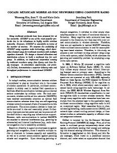
One of the major challenges in forming a grid over ad hoc network is the mobility of the nodes and an infrastructure-less network. Resource identification and sharing become difficult tasks in a mobile environment. To overcome this, we propose a model to identify the stability of the nodes which in turn helps to predict the stability of the grid. The stability of the node is predicted using the TBM model [6]. The TBM model Mobility models are application dependent. Hence application scenarios are important in choosing a model. Although typical application domains of ad hoc networks are military networks, conferences and search/rescue operations, for the kind of grid based sharing of resources, we consider offices and institutions where people meet regularly, with a myriad of heterogeneous mobile devices, as the application domain. In these domains, there exist fair amounts of regularity in the movement of the mobile nodes. Hence as opposed to the former group of applications where the mobility models try to model the randomness in the movement, in our application domain, we are more concerned with capturing the regularity of the movement. Hence we use a mobility model that records regular movements to efficiently manage mobility. TBMM identifies regularity in movement of the nodes and captures them as a movement pattern. Each node is assumed to be location aware, and the network is assumed to be mapped on to a virtual grid structure, depending upon the transmission region and the area of the network. A light-weight algorithm

www.ubicc.org

Ubiquitous Computing and Communication Journal

Grid Resources

Grid Resource Table

Resource management

Resource Discovery

Initiate to form Grid Provider Registration

Resource Parameter, Service Fee, Stability Time, Position Consumer Registration Type of Service, Price, Stability Time, Position

QoS Routing

Negotiation Resource Access Updating Resources Services Monitoring

Stability Time, Position, Queue Size

Fig 1 Architecture of a mobile ad hoc grid [6] is used to arrive at the trace representing the regular movement of the nodes over a period of time. The information in the trace consists of a series of stable positions and associated time duration. We propose a trace-based approach to form a grid over an ad hoc network using the above-mentioned trace. Further, the mobile ad hoc grid uses a lightweight algorithm for grid formation, resource discovery, negotiation, job scheduling, and resource sharing, in keeping with the limited resource characteristic of the mobile nodes. Load balancing is a challenge unique to the dynamic nature of ad hoc network, and it is not considered for the initial study of formation of grid over an ad hoc network. The architecture of the grid is shown in Fig. 1. The grid layer is built on top of a QoS guaranteeing network layer that provides stable routes. The grid layer consists of a grid resources module, resource discovery module, and resource management module. The resource discovery module initiates grid formation, and allows the service providers and consumer nodes to register. Grid resources module maintains and keeps track of the registered resources. Resource management module is responsible for negotiation, resource access, updating of resources and service monitoring. All these modules are built on the QoS routing of network layer, which could in turn make use of the same stability information obtained from the TBMM.

Volume 2 Number 5

Page 79

4

GRID FORMATION

A node willing to provide service with higher computational capability and power is called as a service provider node (SPN) and the node which requests for the service is called as a consumer node (CN). The SPNs and CNs are the members of the grid. The nodes that are willing to share their resources specify a cost for their resources. The consumer node accepts a service based on the cost, service time, etc. This leads to some negotiation between the consumer node (CN) and the service provider node (SPN). Since ad hoc network is an infrastructure-less network, there is no centralized authority to keep track of the negotiation between a CN and a SPN. In order to form a grid and to keep track of the negotiation between a CN and a SPN, we have an SPN that volunteers to act as a grid head node (GHN). The GHN takes care of the negotiation between the CN and SPN. The GHN of a grid acts as a central point and is responsible for resource discovery and resource access. Figure 2 shows the messages that are exchanged between the nodes that are willing to form a grid. Resource Discovery A node that is willing to provide service will initiate the action of forming the grid by sending a grid_hello_message. The nodes that are willing to be a member of a grid respond to the grid_hello_message. The format of grid_hello_message is as shown in figure 3a. It consists of node ID, stability time, position and hop

www.ubicc.org

Ubiquitous Computing and Communication Journal

count. The node ID is the identification of the node that sends the message; and stability time and position which are obtained from its trace file denote the current position and the associated stability time. When two nodes send a grid_hello_message at the same time, the grid head elected is the one that has a larger stability time. Hop count restricts the propagation of the grid_hello_message to a limited number of hops. This helps to avoid the formation of one large centralized grid, and instead facilitates multiple decentralized grid structures. CN

consists of SPN ID, GHN ID, Resource parameter, service fee, Position and Stability. The SPN ID is the ID of the node that is willing to join the grid and GHN ID is the head ID under which it wants to become a member. Resource parameter indicates the resource parameter that is available with a SPN like the computational capability, power, storage etc. The service fee indicates at what cost it will service a request. Similarly a node requesting for service sends a service_request_message whose format is shown in figure 3c. Service_request_message consists of the

SPN

GHN/SPN

Grid_Hello_Message

Grid_Hello_Message

Grid_Joining_Message Service_Request_Message

Service_ Provider_Message / Service Denial Message Seeking_Service_Message Service

Result Message

Acknowledgement Message

Service_Completion_Message

Fig 2 Sequence of messages for Grid formation

Table 1 Grid Table Node

SPN

RP/

Service

ID

/CN

ToS

Fee

Price

Position

Stability

Job

Busy/

ID

Free

Abbreviations: SPN/CN – Service Provider Node/ Consumer Node, RP/ToS – Resource Parameters/Type of Service A node, after receiving a grid_hello_message, sends a response message depending on whether it wants to become a member of the grid or wants to request for service. The node joining a grid sends a grid_joining_message. The format of the grid_joining_message is shown in Figure 3.3b. It

Volume 2 Number 5

Page 80

requesting node ID, GHN ID, ToS, Price, Position and Stability. The GHN is the grid head ID to which it is requesting service. ToS is the type of service requested by a CN. The price field indicates at what price it is willing to accept a service. A node can also become a member of two grids based on the resources available with it or the services it desires.

www.ubicc.org

Ubiquitous Computing and Communication Journal

Service_seeking_message and result_message are not handled here because they both are application dependent. Grid Resources : The GHN after receiving responses from the member nodes forms a grid table. The format of the grid table is shown in Table 1 This table maintains the details about the member nodes. The node ID column lists the identification of the member nodes. The SPN/CN indicates whether it is a SPN or CN. The resource parameters specify the resources available with that node like computational capability, power, storage etc. Type of service indicates what type of service is needed by a CN. Service fee of a SPN specifies at what cost it will service a CN. Price of a CN specifies at what price it needs a service. Position is the physical location of a node and stability is how much time a node is going to be present at that location. Job ID is a unique ID assigned to the communication of a SPN and a CN. Busy indicates whether a node is being serviced in the case of a CN or is providing service in the case of an SPN. Free indicates that an SPN is free to provide service. The head maintains all the details about its members. Resource Management: The head node is responsible for the negotiation between a SPN and a CN. When a node requests for a service it sends the details of what type of service it needs and at what cost. So the head node looks at the table to find out a SPN that offers the service at that cost. Re-negotiation also can be done by a GHN and it is in the pipeline. The job scheduling is done based on the stability time and the location of the SPN. A GHN first verifies, whether the service time of a CN is greater than the stability time of a SPN. If many SPNs have greater stability time, then an SPN that is nearer to the CN requesting for a service is assigned. There may be situations where a GHN sends a service_denial_message based on the available / residual service time. The residual service time is calculated based on the total stability time of SPNs associated with the GHN and the already used up/ committed service time. If the residual service time is less than the service time of the current request then it sends a service_denial_message. The format of this message is given in Figure 3d1. It consists of CN ID, GHN ID, and denied service message where the CN ID is the ID of the node requesting service, GHN ID is the ID of the node sending the message. Otherwise, the GHN sends a service_provider_message to CN. The format of the

Volume 2 Number 5

Page 81

service_provider_message is given in Figure 3d2. It consists of CN ID, GHN ID, SPN ID, Job ID, cost, position and stability. The CN ID is the ID of the node requesting service, GHN ID is the ID of the node sending the message and SPN ID is the ID of the node that has been assigned to provide service. The job ID is a unique ID assigned by GHN to identify the communication between the CN and SPN. Position indicates the physical position of the SPN that has been assigned to the CN. On receiving this message the CN starts communicating with the SPN for its service. The position of the SPN is available in the message, hence the CN can easily communicate with the SPN using the routing protocol in the network layer. After getting the service, the CN sends an acknowledgement about its completion of the service to the GHN. Service completion field indicates that the service is completed. The Job ID is sent so that the GHN can understand which service was completed. The format of the acknowledgement_message is given in figure 3e. Similarly the SPN sends a service_completion_message to the GHN after completing the service for a CN. The format of the service_completion_message is given in Figure 3f. It consists of SPN ID, GHN ID, job ID, WtoC, URP and service fee. The job ID to identify the job that has been completed and if the SPN is willing to continue (WtoC) in a grid it sends the willingness as well as the updated resources parameters (URP) to the GHN. Using this information the GHN will know that the service has been successfully completed and updates the resource parameters of the SPN in its table. The GHN has to periodically send a grid_hello_message to its member nodes, so that the members will know that the GHN is alive, and a new member will also know about the GHN. Since, it is an ad hoc network there might be situations where the members have to leave the grid even before the stability time expires. During this case, the members have to inform the GHN by sending a bye_message that consists of its ID and leaving grid information. The format of bye_message is shown in Figure 3g. Similarly when a GHN leaves the grid, it has to select a new head from its grid table, the new head will be a SPN which has the largest stability time (after ascertaining its willingness to be the new GHN). The GHN informs the members of the grid about the selection of a new head by sending a new GHN message. This message consists of old grid head ID (GHN), new grid head ID (New GHN) as well as the stability time and position of the new grid head. The format is as shown in Figure 3h. The node

www.ubicc.org

Ubiquitous Computing and Communication Journal

Node ID

Stability Time

Position

Hop count

Service Fee

Position

Fig 3a grid_hello_message

SPN ID

GHN ID

RP

Stability

Fig 3b: grid_joining_message sent by SPN

CN ID

GHN ID

ToS

Price

Position

Stability

Fig 3c: service_request_message sent by CN

CN ID

GHN ID

Denied Service

Fig 3d1: service_denial_message sent by GHN CN ID

GHN ID

SPN ID

Job ID

Cost

Position

Stability

Fig 3d2: service_provider_message sent by GHN

CN ID

GHN ID

Job ID

Service Completion

Fig 3e: acknowledgement_message sent by CN

SPN ID

GHN ID

Job ID

WtoC

URP

Service Fee

Fig 3f: service_completion_message sent by SPN

CN/SPN ID

GHN ID

LG

Fig 3g: bye_message

GHN ID

New GHN ID

Stability Time

Position

Hop Count

Fig 3h: New GHN message Abbreviations: GHN ID – Grid Head Node ID, SPN/CN – Service Provider Node/ Consumer Node, RP/ToS – Resource Parameter/Type of Service WtoC – Willing to Continue, URP – Updated Resource Parameters, LG – Leaving Grid

selected as a new head sends a grid_hello_message to its members. The previous GHN hands over the table it maintained to the new GHN. Even when a GHN fails, it is identified by the non-receipt of the grid_hello_message and any SPN can initiate the formation of the grid by sending the grid_hello_message. But this will involve grid formation overhead. Similarly, situations like network splits or networks merge can also be

Volume 2 Number 5

Page 82

handled. When a network split occur the members leaving the grid will inform the GHN by sending a bye_message and the grid will still exists with the available resources. When network merge happens it will not affect the existing grid, instead new members will join the grid. But this situation will not happen frequently in a low mobile scenario. The analysis of mobile ad hoc grid is presented below.

www.ubicc.org

Ubiquitous Computing and Communication Journal

5

MODELLING OF MOBILE AD HOC GRID

The Mobile ad hoc grid is modeled as an M/M/m queuing system [12] in order to estimate the performance. A service request from a CN can be considered as the arrival of a customer in the M/M/m parlance. Thus the service requests from the CNs at a GHN form the arrival process, and the SPNs are the m servers servicing these requests. In keeping with the M/M/m model, the arrival process (with arrival rate λ at a GHN) is Poisson and the service time of the SPNs (with mean 1/µ sec) are independent and exponentially distributed. The successive interarrival times and service times are assumed to be statistically independent of each other. Here we analyze two cases - one is when the SPNs are stationary and the other, when they are mobile. It is assumed that the GHNs are stationary. In this grid, the CNs request for a service to the GHN and the GHN is responsible for assigning an SPN to the requesting CN. Hence, the probability that an arriving request in a GHN will find all servers busy and will be forced to wait in queue is an important measure of performance. Similarly, if a GHN does not have sufficient number of SPNs to assign for the services requested, then also there is a probability of queuing (or waiting). This is irrespective of the SPNs being mobile or stationary. However, if the SPNs are mobile, it is also possible that a CN is denied service since the committed service time of the earlier requests is greater than the stability time of the SPNs. Hence determining the probability of this event is another performance measure considered. . Case I - Static SPNs : When the SPNs are static, the number of servers is fixed. Hence, in the M/M/m model, m (i.e the number of SPNs) is fixed based on the number of servers available. The utilization factor (i.e the proportion of time the server is busy) is calculated as shown in equation (1), ρ= λ /m µ < 1

(1)

The probability of queuing PQ is given in equation (2). PQ = p0(m ρ)m/m!(1- ρ)

(2)

Where p0= [ ∑(m ρ) n/n!+(m ρ)m/m!(1- ρ) ] –1 where n = 1to (m-1)

A request in a waiting state is serviced when a new SPN registers with the GHN or a SPN has completed its service and it is willing to continue in the grid. Duration of time a request has to wait in a queue is known as the waiting time of the customer. Equation (3) gives the average waiting time (W), that a service request has to wait in queue.

Volume 2 Number 5

Page 83

W = NQ/λ = ρPQ/ λ(1- ρ)

(3)

Delay per customer D includes the time taken by a SPN to service the request as well as the waiting time of a request in the queue of the GHN. Equation (4) gives the average delay per customer (which includes service time and waiting time). (4) D = 1/µ+W = 1/µ + ρPQ/(λ(1- ρ)) The number of customers in the system is the total number of requests received by a GHN. Equation (5) gives the average number of customers in the system. (5) N= λD = (λ /µ) + λPQ/(m µ - λ) Case II – Mobile SPNs: Here, since the SPNs are mobile, the number of SPNs associated with a GHN varies with respect to time. Hence to determine ‘m’ of M/M/m model, the average number of SPNs associated to a GHN has to be calculated. We proceed as follows to determine this value. Let us assume that there are n SPNs in a grid. Let p1 Æ probability of SPN1 being in a given GHN, p2 Æ probability of SPN2 being in it …. pn Æ probability of SPNn being in it pi may be calculated based on the time duration for which it is associated with the GHN. This is obtained from the movement trace pattern followed by the nodes. To find out the average number of SPNs (AVSPN) associated with a GHN, first we have to find out the probability of number of SPNs associated with a GHN. Equations (6) to (8) give the probability of the number of SPNs being associated with a GHN. Let, q1 Æ probability that atleast one SPN has been associated with a GHN q2 Æ probability that atleast two SPNs have been associated with a GHN … qn Æ probability that all the n SPNs have been associated with a GHN q1 = p1(1- p2)…(1- pn) + p2(1- p1)…(1-pn) + … + pn(1-p1)…(1-pn-1) (6) q2 = p1p2 (1- p3)…(1- pn) + p1p3 (1- p2)…(1- pn) + (7) … + p n-1 pn (1- p1)…(1- pn-2) …. (8) q n = p 1 p 2 … pn Then, the average number of SPNs (AVSPN ) associated with a GHN is obtained as shown in the equation 9 ,

www.ubicc.org

Ubiquitous Computing and Communication Journal

AVSPN = Σiqi, where i varies from 1 to n (9) Averaging this value over the number of SPNs available gives an estimate of m. Next, we have to determine the number of requests that are denied service. This is because the SPNs are mobile. Towards this, we first calculate the available / residual service time by subtracting the already used up service time from the total stability time of SPNs as shown in Equation (10). Residual service time = Total stability time of SPNs – already used up service time (10) Tres = m(T – t) - λt /mµ where T is the total stability time of an SPN, t is the time at which the request arrives and m is the average number of SPNs. The condition for service denial is that this residual service time is less than the service time of the current request as shown in equation (11). m(T-t) – ( λt /mµ) < 1/µ (11) Rearranging, we get the arrival time t after which service will be denied as t ≅ (m2µT – m) / (m2 µ+ λ) (12) Limiting this by the stability time T, we get (13) t ≅ min(T, (m2µT – m) / (m2 µ+ λ)) Hence, the number of requests that will be denied service (NDS), is the number of requests that arrive in the time T-t and is given in equation (14). (14) NDS = (T-t) λ . The arrival rate decreases to λnew, due to NDS number of request being denied of service. The λnew is calculated as shown in equation 15. λnew ≅ (λt-Nds)/T

(15)

where λt is the total number of requests that arrive, NDS is the number of requests that are denied service and T is the total stability time of an SPN. Using m and λnew the equations (1) to (5) may be used to determine the various performance measures. In this case, we replace λ by λnew The next section presents the details of the simulation that has been carried out to validate the proposed architecture and this model. 6. Performance Evaluation through Simulation Simulation studies have been carried out to evaluate the mobile ad hoc grid architecture. The simulation

Volume 2 Number 5

Page 84

tool used is Glomosim [11]. The parameters used for the simulation are given in Table 2. The mobility model used for the nodes is a trace-based model derived from Ansim [13] depicting a University scenario. Table 2 Parameters for the simulation Number of Nodes

50

Simulation Time Terrain Dimension Mobility

1000 Seconds (1000,1000) meters

Radio-Tx-Power MAC-Protocol Routing Protocols

Mobility Trace, Mobility-Trace-File 8 dBm (with a reach of 250 meters) 802.11 TBSR-Q

A Mobile ad hoc grid has been simulated in this set up using 4 GHNs and 12 SPNs. Here the GHNs are considered to be static. The results are separately analyzed for the two cases, namely, static SPNs and mobile SPNs. For the given trace information, when the SPNs are static, the average number of SPNs associated with a GHN is 3 whereas when they are mobile, the average number of SPNs per GHN is 2. To analyze the performance of the grid, the parameters of interest are average time a customer has to wait in queue, average delay per customer and the overhead in forming the grid. The performance is analyzed by increasing the number of consumer nodes from 4 to 20 in steps of 4 (with an average of 1 to 5 CNs per GHN) that in turn will increase the number of service requests. Figs 4a and 5a shows the average time a customer has to wait in queue when SPNs are static and mobile respectively. The avg. waiting time increases as the number of service requests increases. this is because sufficient number of SPNs are not available to service the request. When we compare the avg. waiting time of the static SPNs and mobile SPNs there are variations in the avg. waiting time. This is due to variation in the number of SPNs getting associated with a GHN. Figs 4b and 5b show the average delay per customer, when SPNs are static and mobile. These results are reflected by the avg. waiting time in the queue. Fig 5c shows the average number of request denied service when SPNs are mobile. The situation arises only when the residual service time of a GHN is lesser than the service time of the current request. The simulation results matches

the expected

www.ubicc.org

Overhead in forming a grid : The overhead in forming a grid is comprised of additional grid-forming messages that are communicated among the nodes to form the grid and the average routing delay. Figures 6 a, b and Figure 7 a, b show the control message overhead and the average routing delay when SPNs are mobile and static. In the case of mobile SPNs the control message overhead is more compared to the static SPNs. This is because the mobile SPNs leave one GHN and join another GHN when they are moving. Average routing delay considers the delay in routing the control packets at the network layer. However, the average routing delay increases as the number of CNs increases; this is due to the increase in the number of service requests. But the routing delay caused due to the mobile environment is very less and does not affect the performance of the mobile ad hoc grid.

Simulation Result Theoretical Result

25 20 15 10 5 0 4

8

40 30 20 10 0

16

20

b: Average Delay per Customer when SPNs are mobile

3 2 1 0 8

12

16

20

Average Time a Customer has to Wait in Queue when SPNs are static

Avg. No. of Request Deined Service

Avg. Waiting Time per GHN (Sec)

12

No. of Consumer Nodes

No. of Consumer Nodes

6 5 4 3 2 1 0

Simulation Result Theoretical Result

4 30 Avg. Delay Per Customer (Sec)

8

4

4

a.

20

Simulation Result Theoretical Result

50

Simulation Result Theoretical Result

5

16

a: Average Time a Customer has to Wait in Queue when SPNs are mobile

4 6

12

No. of Cons um e r Node s

Avg. Delay Per Customer (Sec)

theoretical results.

Avg. Waiting Time (Sec)

Ubiquitous Computing and Communication Journal

Simulation Result Theoretical Result

8

12

16

20

No. of Consumer Nodes

25

C: Average No. of Request Denied Service when SPNs are mobile

20 15 10

Fig 5 Mobile SPNs

5 Avg. No. of Control Messages

0 4 8 12 16 20 No. of Consumer Nodes

b: Average Delay per Customer when SPNs are static

1200 1000 800 600 400 200 0 4 8 12 16 20 No. of Consumer Nodes

Fig 4 Static SPNs

a: Control Message Overhead when SPNs are static

Volume 2 Number 5

Page 85

www.ubicc.org

Avg. Routing Delay (Sec)

Ubiquitous Computing and Communication Journal

using these devices.

0.6 0.5

7.2 Applicability to Wireless Mesh Network :

0.4 0.3

The mobile ad hoc grid architecture proposed can be easily applied as an overlay in Wireless mesh network (WMN) [14] scenarios. Typically, a WMN consists of two types of nodes, mesh routers and mesh clients. The mesh nodes constitute the members of the grid, with mesh routers playing the role of GHNs and SPNs, and mesh clients acting as CNs. Since the mesh routers usually have minimal mobility and are not limited in terms of resources, they suit the role of GHNs and SPNs. Since the mesh clients may be stationary or mobile, depending on their capability, they may act as clients only or as SPNs as well. The GHNs and the SPNs acts as backbone nodes for the grid formation and deliver the requested service.

0.2 0.1 0 4

8

12

16

20

No. of Cons um e r Node s

b : Average Routing Delay when SPNs are static

Avg. No. of Control Messages

Fig 6 Overhead for Static SPNs 1500 1000

8 0 4

8

12

16

20

No. of Cons um e r Node s

a: Control Message Overhead when SPNs are mobile Avg. Routing Delay (Sec)

CONCLUSION AND FUTURE WORK

500

This paper has proposed an architecture to form a grid over a mobile ad hoc network by using trace files that capture the regularity in the movement or rather the stability of the nodes. It has also shown the feasibility of sharing the resources using such a grid by proposing a theoretical model and simulation studies. Further issues to be explored are building trust over the mobile ad hoc grid and mechanisms for the cooperation of nodes to share their resources.

0.8

ACKNOWLEDGMENT

0.6

The authors would like to thank Dr. V.Uma Maheswari for her valuable suggestions during the analysis process of mobile ad hoc grid.

0.4 0.2 0 4

8

12

16

9

20

No. of Cons um e r Node s

b : Average Routing Delay when SPNs are mobile Fig 7 Overhead for Mobile SPNs The performance of the mobile ad hoc grid shows the feasibility of forming a grid in a mobile environment. 7. Application scenarios 7.1 Applicability to Ad Hoc Network In a regular ad hoc network, devices like highend Laptop PCs, Low-end Laptop PCs can be a GHN or SPN, whereas PDAs, pocket PCs, mobile phones etc., can be a CN. Wireless Grid can be formed

Volume 2 Number 5

Page 86

REFERENCES

[1] I.Foster, “What is the Grid? A Three Point Checklist”, GRID Today, July 20, 2002 [2] Open Grid Services Architecture http://www.globus.org/ogsa/ [3] David P. Anderson, “BONIC: A system for Public-Resource Computing and storage”, 5th IEEE/ACM International Workshop on Grid Computing, Nov 2004. [4] Thomas Phan, Lloyd Huang, Chris Dulan, “Challenge: Integrating Mobile Wireless Devices into the Computational Grid”, IEEE/ACM International Conference on Mobile Computing and Networking (MOBICOM) 2002. [5] Jing Su, Alvin Chin, Anna Popivanova, Ashvin Geol, Eyal De Lara, “User Mobility for Opportunistic Ad-hoc Networking”, Proceedings of Sixth IEEE Workshop on Mobile Computing Systems and Applications(WMCSA’04)-Volume 00, 41-50, Dec 2004.

www.ubicc.org

Ubiquitous Computing and Communication Journal

[6] V.Vetri Selvi and Ranjani Parthasarathi, “Trace Based Mobility Model to Support Quality of Service in Ad Hoc Networks ”, Trusted Internet Workshop (TIW05) held along with 12th International Conference on High Performance Computing (HiPC2005), 18-21 Dec. 2005. [7] Imran Ihsan, Muhammed Abdul Qadir, Nadeem Iftikhar, “ Mobile Ad- Hoc Service GridMASGRID”, Third World Enformatika Conference, WEC'05, pp 124-127,April 2005. [8] Zhi Wang, Bo Yu, Qi Chen, Chuanshan Gao, “Wireless Grid Computing over Mobile Ad-Hoc Networks with Mobile Agent”, First International Conference on Semantics, Knowledge and Grid, Nov 2005. [9] J. Anda, J. LeBrun, D. Ghosal, C-N. Chuah, and H. M. Zhang, "VGrid: Vehicular Ad Hoc Networking and Computing Grid for Intelligent Traffic Control," IEEE Vehicular Technology Conference, Spring 2005. [10] Roy, N. Das, S.K.Basu, K.Kumar M, “Enhancing Availability of Grid Computational Services to Ubiquitous Computing Applications”, 19th IEEE International Symposium on Parallel and Distributed Processing, April 2005. [11] http://pcl.cs.ucla.edu/projects/glomosim, 2000. [12] Dimitri Bertsekas, Robert Gallager, “Data Networks”, 2nd Edition, Prentice-Hall India pp 174-176,1999. [13] http://www.i-u.de/schools/hellbrueck/ansim [14] Ian F.Akyildiz, Xudong Wang and Weilin Wang, “Wireless mesh networks: a survey”, International Journal of Computer and Telecommunication Networking, volume 47, Issue 4, pages 443-598, March 2005.

Volume 2 Number 5

Page 87

www.ubicc.org