Mobility-assisted Hierarchy for Efficient Data Collection in Wireless ...

JOURNAL OF COMMUNICATIONS, VOL. 5, NO. 9, OCTOBER 2010

665

Mobility-assisted Hierarchy for Efficient Data Collection in Wireless Sensor Networks Zuzhi Fan College of Information Science & Technology, Jinan University, China Email: [email protected] Yuanzhu Peter Chen Department of Computer Science, Memorial University of Newfoundland, Canada Email: [email protected]

Abstract— One fundamental task of wireless sensor networks (WSNs) is to collect useful information from the sensory field or response users query. In such scenario, the gigantic amount of individual sensor readings will converge to the base station (BS) of the network. Thus, the “funnelling effect” which describes the convergence of data traffic towards data sinks remains a major threat to the network lifetime. In particular, those sensors near data sinks need to relay data for nodes that farther away and burn energy faster with the result that the network may become disconnected or dysfunctional. In this paper, we investigate a heterogeneous sensor network by introducing a few mobile elements1 , referred as aggregators into static sensor network and utilize the mobility to alleviate the ”funnelling effect”. In particular, these aggregators deploy themselves and worked as cluster heads. In such mobility-assisted hierarchy, we study the aggregator deployment problem for energy conservation and consider the integration of mobility and routing algorithms for lifetime elongation. Based on the extensive simulation, we show that such mobility-based hierarchy can significantly mitigate the ”funnelling effect” and then prolong network lifetime. Index Terms— wireless sensor network, data collection, mobility, deployment

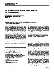
I. I NTRODUCTION A typical application mode of wireless sensor networks, referred as continual data gathering [1] is that the nodes within sensory field collect information periodically and then transmit it to the BS, which is characterized by manyto-one traffic pattern, i.e., all traffic in the network will converge to the BS. In a homogeneous network, where sensors are organized into a tree topology (Figure 1(a)), sensors far away from BS often send packets in a multihop fashion for energy consideration. Obviously, those sensors near the BS need to forward more packets and This paper is based on “Prolonging Lifetime via Mobility and Loadbalanced Routing in Wireless Sensor Networks” by Zuzhi Fan, which appeared in the Proceedings of 2009 IEEE International Symposium on c IEEE. Parallel&Distributed Processing, pp. 1-6, 2009. ° Manuscript received February 13,2010; revised March 10,2010; accepted May 31,2010. Email:[email protected] 1 As above, the words mobile aggregator, mobile element, mobile base stations, mobile sink are used interchangeably. They all mean mobile nodes with abundant resource.

© 2010 ACADEMY PUBLISHER doi:10.4304/jcm.5.9.665-673

become heavy-loaded. If the BS is located at the center of sensor field, the “funneling effect” of energy dissipation appears. As a result, such an uneven use of energy may cause some nodes within ”hot spot” to fail, thus create holes in the network or worse, leave the network disconnected(Figure 1(a)). Many algorithms and protocols have been proposed to the problem in terms of routing strategies [2], data aggregation and network self-configuration [3]–[6]. An effective way is to organize the network into hierarchical or multi-layers architecture [3], [5]. In such kinds of approach, a few sensors are elected as cluster-heads to collect data from their neighboring nodes and relay them to the BS (Figure 1(b)). To conserve energy, cluster-heads will aggregate the received data before forwarding them. Also, those cluster-heads will be selected periodically to avoid over-loading themselves. As a matter of fact, the hot spots have been diffused across the network along with cluster-heads shift. However, the hierarchical architecture can be inefficient with the drastically increasing of network scale. In very large scale networks, the selected cluster-heads tend to be overloaded and thus drained of their battery power quickly. Though the re-clustering strategy may alleviate the problem, it will increase the cost of cluster maintenance. Multi-layers organization can be another alternative. However, the clustering process can be extremely complicated with the growing in number of layers [7]. Intuitively, it is possible to balance the load of sensor nodes if BSs or cluster-heads change their position from time to time, which is analytically proved by [8] and our prior work [9]. In this paper, we consider a heterogeneous network which consists of a few mobile aggregators with sufficient power supply and large number of resourceconstrained static sensors [10]. Based on the architecture, we propose a mobility-assisted hierarchy where mobile elements work as the cluster heads and collect sensed data from sensors via multi-hop communication. In the scenario, the “funneling effect” is taken place around the mobile cluster-heads. To distribute energy consumption evenly, mobile elements will move periodically [11]. In a summary, the network lifetime is split into equal periods of time know as rounds. Mobile elements relocate at the

666

JOURNAL OF COMMUNICATIONS, VOL. 5, NO. 9, OCTOBER 2010

Hot spot

BS

BS

Sensor node

Heavy-load nodes

(a)Flat routing scheme

Sensor nodes

Heavy-load nodes

(b)Cluster-based routing scheme

Figure 1. “Funneling effect” in wireless multi-hop communication. The residual energy level of sensors is indicated by different color depth. Dark color means less available energy or vice versa.

begin of each round and then stay static in the rest round. The following data gathering process is similar as the stationary sink [3]. Such a “move and sojourn” strategy can balance the energy consumption among sensors, but two issues should be exploited [12]–[15]: (1) How do we determine new locations for the mobile elements to conserver energy? (2) What is the efficient communication mode between mobile elements and sensors [16]? Our contributions in this paper include: (1) We investigate data gathering schemes supported by mobility and make a comparison in terms of network environment, mobility strategies and routing algorithm. (2) From the perspective of comparison, we propose both centralized and distributed aggregator deployment protocols for presented hierarchy, which can be proved very energy-efficient. (3) At last, the effective integration of mobility with different routing strategies is studied to further prolong the network lifetime, which is validated by extensive simulations. The rest of this paper is organized as follows: In Section II, related work on data collection via mobile elements in WSNs is reviewed. In Section III, we give the problem definition and review proposed scheme in our prior work [9]. Section IV discusses an adaptive deployment protocol and implementation details. Simulation results are provided in Section V. Finally, Section VI concludes the paper. II. RELATED WORK Previous work focused more on static sensor networks and related energy conserving protocols [17]. In a different direction, mobility in sensor networks is firstly described by Tilak et al [1] and extensively discussed by Ekici et al [11]. These approaches exploiting mobility for data collection can be classified as two classes with respect to the properties of sink mobility as well as communications mode. In the first class, mobile elements collect buffered information from sensors by visiting them individually, which is applicable to sparse WSNs [18]– [20]. This kinds of approach can lead to significant delay of data delivery. Therefore, their main issue is to decide the moving trajectory and scheduling in real time to prevent data loss for buffer overflowing. Existing mobility patterns in such scenario include random, fixed and controlled. In [19], assuming that a prototype is built at the Rice University where university shuttle

© 2010 ACADEMY PUBLISHER

buses will carry mobile observer as data sink and sensor nodes are deployed on buildings, the authors model the data collection process as queuing system and propose a communication protocol based on predictable mobility pattern of the observer. Differ from these approaches, we focus attention on the evenly consumption of sensor nodes and network lifetime elongation rather than transmission delay in large scale sensor field. Based on the single Data Mules, David Jea etc. investigated the multiple mobile elements problem for data collection in [13]. Assuming that mobile elements move in the fixed path along a straight line, they study the impact of moving speed and partition of network area rather than location. The other kinds of mobility scheme execute in a “move and sojourn” strategy where mobile elements deploy themselves first and then collect sensed information via spanning routing tree [8], [9], [14], [15]. Finding the optimized deployment position for mobile elements and the appropriate routing path for sensors are the key issues to assure energy efficiency of network. In both [14] and [15], Integer Linear Programming (IPL) model are used to determine the feasible locations of mobile BSs. The difference is that the former aims at the overall network lifespan but the later is to minimizing the energy consumption of individual sensors. However, almost all these approach are executed in a centralized way and the scalability of algorithm is limited. For example, the network considered in [14] is composed of 256 nodes upmost. Our work is particularly motivated by the research in [8], [21], [22]. In [8], the authors developed an analytical model to describe the communication load distribution in wireless sensor networks. It demonstrates that the optimum movement strategy for mobile BS is to follow the periphery when the deployment area is circular. To further alleviate the “funneling effect”, a heuristic solution with mobility and routing algorithm joint is discussed. The simulation results show that such a joint can balance the load among sensors and provide significant improvements on network lifetime in comparison with static BS. However, the mobility strategy may be incapable without assumed Poisson distribution of sensor nodes. We consider the framework with multiple mobile elements rather than single BS in this paper. Moreover, we propose a self-adaptive moving strategy without re-

JOURNAL OF COMMUNICATIONS, VOL. 5, NO. 9, OCTOBER 2010

quirement for the sensors distribution and network shape. In [21], a mobile enabled sensor network supported by the cellular network is presented. Our work differs in that we assume an idealized moving pattern without sink velocity consideration. As a summary, the comparison of these schemes is listed in Table I. At last, a similar mobility-based hierarchy is discussed in [22]. However, it aims to achieve the tradeoff between packet delay and energy dissipation of sensors rather than the optimized deployment of mobile data collectors. III. AGGREGATOR DEPLOYMENT ALGORITHM FOR ENERGY CONSERVATION In this paper, we consider a heterogeneous sensor network which consisted of large number of static resourceconstrained sensor nodes and a number of mobile resource-rich devices, called mobile aggregators (MAs). This mobility-base architecture is demonstrated in Figure 2. In the scenario, we assume a similar application model as described in [3]. That is, each sensor periodically senses the environment and then transmits the received data to the BS. In particular here, each sensor selects the nearest MA as its cluster-head and periodically sends data to the aggregator by multi-hop paths [3]. Next, the aggregators compress the collected data from all members and send the fused data to the BS. 100

80

60

40

20

0

−20

−40

−60

−80

−100 −100

−80

−60

−40

−20

0

20

40

60

80

100

Figure 2. The network hierarchy (Circle denotes sensors, star denotes MAs)

In above architecture, mobile aggregators work as the cluster-heads and relay the received data to remote base station. However, the ”funneling effect” described in section I will emerge near aggregators in large network since sensors burn energy faster than those of nodes father. For load-balanced consideration, MAs should approach areas with higher residual energy among sensors. Our objective is to decide the optimal moving strategy of each aggregator so that the energy consumption in sensor nodes is evenly distributed and the lifetime of network is prolonged. In this section, we first introduce some assumptions and notations in Table II, then bring forward the assumed network model and formulate the problem. Next, we give a skeleton of ADPEC [9], which is a centralized © 2010 ACADEMY PUBLISHER

667

deployment algorithm for energy conservation based on artificial potential-field theory. A. Network Model & Problem Formulation First, we assume that those MAs are equipped with sufficient power and can send fused data to the data sink using out-of-band channels. Thus, the problem can be simplified such that we only need to consider the energy consumption of sensors. We make the following assumptions for the network: 1) We assume a relatively large and strongly connected network, which consisted of k mobile aggregators and a set of (n) static sensor nodes (k ¿ n). As shown in Figure 2, sensors are randomly scattered within a circular field with radius a. 2) The transmission radius of each sensor nodes is identical and fixed at r. 3) There exists a contention free MAC protocol which provides channel access to all the nodes. 4) Each sensor is aware of the residual energy of its neighboring nodes by overhearing at anytime. 5) We consider equal period of time called round. At the start of each round, MAs relocate themselves as per specific deployment protocol and stay fixed during the round. Based on the assumptions, the whole network will be divided into a few clusters encircled MAs. In fact, each sensor will select the nearest MA to join and the network is formed as Voronoi diagram (Figure 2). Since MAs is much fewer compared to sensors, nodes faraway from cluster centre have to communicate with MAs by dedicated multi-hop routing algorithm, such as CDPR [9]. Inevitably, the “funneling effect” will bring the uneven energy dissipation among the sensor nodes. Therefore, two important issues in the context should be addressed: 1) The mobility strategy: How to move MA to their optimal position at the start of each round so that the energy consumption of sensors will be balanced? 2) The routing algorithm: Though routing can not get rid of the “funneling effect”, a load-balanced routing algorithm will make the energy consumption more even. B. Potential-field based approach The first issue discussed above is similar to finding the optimal positions for cluster-heads in [3], which has proved to be NP-hard. In our prior work [9], a potentialfield-based deployment protocol, named ADPEC is proposed to deploy MAs periodically. Meanwhile, a nearstraight routing protocol accompanied with ADPEC is used in the communication between sensors and aggregators. The system parameters used are listed in Table II. In ADPEC, both sensors and MAs are imaged as virtual particles in the artificial potential field. Each aggregator is attracted by all sensors of the network and repelled by near aggregators. The attractive potential exerted on aggregator Ai at position q is proportional to the residual

668

JOURNAL OF COMMUNICATIONS, VOL. 5, NO. 9, OCTOBER 2010

TABLE I. C HARACTERISTICS OF DATA GATHERING SCHEMES WITH MOBILITY

Infrastructure

Scheme

Number MEs

of

Moving Strategies

Topology

Pattern

Trajectory

Algorithm Execution

Routing Path

Predicable Observer Mobility [19]

Single

Disconnected

Continuous

Fixed

None

Single-hop

PBS [11], [12]

Single

Disconnected

Continuous

Controlled

Centralized

Single-hop

Data Mule [18]

Multiple

Disconnected

Continuous

Random

None

Single-hop

MES [20]

Single

Disconnected

Continuous

Controlled

Centralized

Single-hop

Sojourn [14]

Single

Disconnected

Continuous

Controlled

Centralized

Single-hop

Data Mules [13]

Multiple

Connected

Discrete

Fixed

Distributed

Multi-hop

BSL [15]

Multiple

Connected

Discrete

Controlled

Centralized

Multi-hop

Joint Mobility and Routing [8]

Single

Connected

Discrete

Fixed

None

Multi-hop

ADPEC [9]

Both

Connected

Discrete

Controlled

Centralized

Multi-hop

TABLE II. L IST OF N OTATION

Symbol a dchar n k ei e0 eavg d0 UA,i (.) UR,i (.) UT,i (.) ξ η

Meaning Radius of the network deployment region Characteristic distance Number of sensors Number of mobile aggregators The residual energy of sensors Si The initial energy of sensors The average residual energy of all sensors The influence distance of repulsive potential Attractive potential field induced by sensor Si Repulsive potential field induced by aggregator Ai Total potential field experienced by aggregator Ai Scaling factor of attractive potential field Scaling factor of repulsive potential field

energy of sensors and the Euclidean distance between them, which can be described as follows (Eq. 1). UA (q) =

n X 1 i=1

2

ξei d2(q)

(1)

As Eq. 1 described, sensors with more energy level will relay more packets by attracting aggregator to their proximity. On the other hand, the repulsive potential exerted on aggregator Ai by Aj is related to the distance among them (Eq. 2), which will drive them to scatter around the network field evenly. ½ 1 1 − 2 η( d(q) − d10 )2 d(q) ≤ d0 UR,j (q) = (2) 0 otherwise The total potential field experienced by aggregator Ai at position q is: X UT,j (q) = UA (q) + UR,j (q) (3) i6=j

Under the influence of above total potential, the aggregators approach evenly to those nodes with more energy © 2010 ACADEMY PUBLISHER

Objective

Minimizing data loss for buffer overflow

Conserving sensors energy then prolonging network lifetime

level. As the total potential exerted is minimized, the aggregators will find the optimal deployment. Assumed that the aggregators are equipped with sufficient power or rechargeable, deployment algorithm is performed by aggregators in ADPEC. As described in Eq. 1, the attractive potential UA (q) can be calculated provided that the aggregator Ai acquires the residual energy level and positions of all sensors; while the positions information can be obtained by aggregators at the bootstrap phase of network. In the implementation of ADPEC, we assume that sensors piggyback energy information on sensed data to their aggregators. However, the information of residual energy level should be exchanged among all sensors in each deployment, which may be non-scalable in largescale networks. The solution to the second issue in Section III-A is routing algorithm. In ADPEC, a near-straight routing algorithm, named CDPR is proposed to accompany with deployment protocols. That is, each sensor forwards the received packet to the next hop which is dchar away from the current node and on the way to its destination. In that way, the energy consumed by each sensor will be minimized and total energy consumption of network is minimized, while CDPR may not lead to maximum network lifetime [23]. IV. L OCALIZED AGGREGATOR D EPLOYMENT P ROTOCOL AND L OAD - BALANCED ROUTING A LGORITHM As discussed in section III-B, a centralized deployment protocol, named ADPEC [9] is proposed. Meanwhile, a near-straight routing protocol, called CDPR is used in the communication between sensors and aggregators. However, the calculation of attractive potential field in ADPEC is based on the global information, such as energy level and position of sensors. Obviously, it is energy

JOURNAL OF COMMUNICATIONS, VOL. 5, NO. 9, OCTOBER 2010

TABLE III. L IST OF N OTATION

Symbol he,i h0 di wi Ci N (Si )

669

B. Load-balanced Routing algorithm

Meaning The hop count from sensor Si to cell border The influent distance of repulsive potential The distance from sensor Si to its aggregator Ai The routing weight of sensor Si The set of sensors covered by aggregator Ai The set of neighboring sensors for Si

consuming and non-scalable in large-scale networks. On the other hand, we observe that under the assumption of circular deployment and uniformly distributed network, the trajectory of MAs is approximate to be concentric circles around the network center, which ignite us to promote a localized deployment protocol. The notations used in the section is listed in Table III.

Routing is another effective way to relieve ”funneling effect” and conserve energy in sensor networks. A near-straight routing algorithm, Characteristic Distance Progressive Routing (CDPR) is proposed coming with ADPEC to minimize total energy consumption. As simple topology shown in Figure 3, the total amount of energy dissipated would be minimized only when the sender (at s) relays packets to the receiver (at d) by multi-hops path and each hops is exactly dchar [24]. Here, the distance dchar depends on the hardware parameters of nodes.

Figure 3. Characteristic Distance (dchar )

A. Distributed Deployment protocol In the section, a localized potential-based deployment protocol, named LADPEC is presented. In LADPEC, the network is divided into many Voronoi cells centered at the MAs. Differing from ADPEC, the topology will keep stable in spite of MA mobility. In other words, each MA serves the fixed number of sensors within its covered cell. Then, each MA is attracted by the sensors within its Voronoi cell and repelled by the cell border. Supposing aggregator Aj is at position q within the cell Cj , the potential exerted by sensor node Si depends on its hop count to cell border he,i . If he,i is larger than h0 , the sensor Si will exert attractive potential described as a scalar function as Eq. (4). UA,i (q) = ei /hi

(he,i > h0 , Si ∈ Cj )

Based on the above conclusion, each packet in CDPR travels along the shortest path to the aggregators and each hop is approximate to dchar (Figure 4), total energy consumption in whole network is minimized. However, the energy consumption in CDPR is not always loadbalanced. As shown in Figure 4, if sensor s and s0 transmit data to d, the routing paths taken by CDPR is s, v1 , v2 , v3 , v4 , d and s0 , v2 , v3 , v4 , d respectively. Obviously, some sensors such as v2 , v3 , v4 are heavily loaded and more energy-consuming. As a result, the partition may lead to the dysfunction or disconnected of network. dchar

s t

(4)

+ v1

Otherwise, the sensor will exert repulsive potential on Aj as Eq. (5).

s’ v2

v3

UR,i (q) = −ei /hi

(he,i ≤ h0 , Si ∈ Cj )

(5) d

Here, ei is the residual energy of sensor Si , hi is the hop count from Si to q and h0 is system parameter describing the influence distance of repulsive potential. At last, the total potential field exerted on aggregator Aj is calculated as Eq. (6). UT =

X

UA,i + UR,i

(Si ∈ Cj )

(6)

Si ∈Cj

The positions with maximum potential field are the optimum position of MAs. To do that, each MA needs to search its own served space locally. The algorithm execution of LADPEC protocol depends on the residual energy and position of sensors in the current cell. Therefore, the protocol is fully self-adaptive without requirement for the network shape and sensors distribution irrespective of the given circular field and random distribution in Section IIIA. © 2010 ACADEMY PUBLISHER

v4

Figure 4. Characteristic Distance Progressive Routing (CDPR)

In this paper, an idealized Load-Balanced Short Path Routing algorithm, shorted as LBSPR is addressed, in which each node decides next hop locally. LBSPR works as follows: Each node Si keeps track of N (Si ), the list of neighboring nodes and their routing weight, wi , which is defined as: wi = ei /di

(7)

Here, ei is the residual energy and di is the distance between sensor Si and its MA. When node Si receives a new packet with destination d, it checks if d is within its communication range. If it is, Si simply sends the request to d directly. Otherwise, Si sends the packet to

670

JOURNAL OF COMMUNICATIONS, VOL. 5, NO. 9, OCTOBER 2010

the node with maximum distance along the right direction in the communication range. If all nodes in N (Si ) have the same energy level, i.e. the initial energy, then Si sends the packet to the furthest node in N (Si ). In this case, LBSPR works as same as shortest path routing, in which sensors choose the furthest node as next hop regardless of the energy distribution within its neighbor. Otherwise, the sensors send the packets to the node with largest routing weight within its neighboring nodes. Figure 5 illustrates this algorithm. Assuming nodes v1 , v2 , v5 , v6 are within the range of s0 and v2 is the nearest node to the destination d, node s0 will select v6 instead of v2 as its next hop because sensor v2 has the lower residual energy and routing weight. Finally, the routing path taken by LBSPR is s, v1 , v2 , v3 , v4 , d and s0 , v6 , v7 , v8 , v4 , d. We can see that only node v4 is the heavily load sensor and the energy consumption has been evenly dispersed. dchar

s t

+ v1 s’ r

v2

v3

d

v6

v5

v7

v4 v8

Figure 5. Load-Balanced Short Path Routing (LBSPR)

C. The Scheme with joint mobility and routing algorithm In this section, aforementioned deployment and routing strategies are taken into account to prolong the network lifetime in mobility-assisted framework. The network lifespan is divided into iterative rounds and each round consists of deployment, routing-establish and data collection phase. The scheme is presented as follows. 1) Initialization. At first, the MAs will self-deploy themselves so they can evenly diffuse over the network. In the stage, Voronoi-based techniques can be used in uniform distribution [25]. Otherwise, ADPEC can be used [9]. After bootstrap, the MAs will broadcast their position information and then sensors choose nearest one as cluster-heads in terms of distance or received signal strength. According to the observation in [9], aggregators move around the concentric circles in uniform network. In LADPEC, we assume that sensors would not change their affiliated MAs even in whole lifetime. Therefore, the network will be partitioned into a few regions, each of which can be served by one aggregator. 2) Deployment. The above deployment algorithm, LADPEC is performed by MAs. To calculate the total potential field, each MA needs to know the energy and position information of sensors within the cell. To conserve energy, the energy level of sensors © 2010 ACADEMY PUBLISHER

can be obtained by piggybacking to the transmitted data. The position information of sensors is used for evaluation of hop counts, but not necessary. Since MA can broadcast “heartbeat” message at radius(r), the sensors received will update their hop count to MA greedily. After finding the optimum position, the aggregator will move there instantaneously and announce its new position. 3) Routing Setup. Once the MAs are deployed, the routing path can be built offline by sensors or MAs. Given the whole topology is known, each MA can figure out the routing path with concentrated computation, which is energy-conserving for sensors but non-scalable. On the contrary, each sensor can set up the route by the position of MAs in a localized way. To do that, each sensor only need to exchange control message with its neighboring nodes. 4) Data Collection. The MAs stay static in this phase. Data collection is performed as same as other protocols, such as LEACH [3]. Sensors send the collected data periodically to their MAs with specified routing algorithm. In our implementation, no aggregation model is considered. Since MAs are not resourceconstrained, we focus only on the communications between nodes and MAs. In practice, this process should last longer than the deployment and routingsetup stage for energy consideration. At last, it might also be noted that the initialization may be performed in a global way. However, the process only initiates at the startup stage, thus the energy consumption in topology discovery is acceptable. V. EXPERIMENTAL METHODOLOGY AND EVALUATION In this section, we do not intend to conduct a complete network-level simulation but an idealized simulation. One reason is that there are nontrivial challenges on mobility and a cross-layer design, in particular, on the interaction of the MAC layer with the networking layer. Such issues are beyond the scope of this paper. The other reason is that the scalability of most network simulators is limited. For example, we have validated that the number of sensors supported by famous Network Simulator 2 [26] is no more than 500 without optimization. However, the network scale in this section can be thousands. Therefore, we perform the experiments with our customized simulator written in C++. A. Simulation Methodology As described in Section II, most of work [11], [12], [14], [19], [20] (as shown in upper of Table I) is focused on the latency of data delivery, which differs from our objective to save energy. Other schemes [8], [13], [15] can be comparable. Simulations in [13], [15] are limited in the size and scale of network. Therefore, we compare our deployment protocols with the convincing scheme (shorted as PERI next) presented in [8].

JOURNAL OF COMMUNICATIONS, VOL. 5, NO. 9, OCTOBER 2010

400

300

200

0 0

100

200

300

Time(# Rounds)

(a) ADPEC

(8) (9)

Where α11 is the energy consumed by the transmitter electronics per bit, α2 accounts for energy dissipated in the transmit amplifier and α12 is the energy consumed by the receiver electronics. Here, the values for radios are α11 = α12 = 50nJ/bit and α2 = 10pJ/bit/m2 . The experiment parameters are listed in Table IV.

Nodes with Residual Energy 0.8~1.0J

100

Nodes with Residual Energy 0.6~0.8J 500

The number of sensors(#)

Etx = α11 + α2 dn Erx = α12

Nodes with Residual Energy 0.6~0.8J 500

The number of sensors(#)

To show how the proposed schemes outperform the others, we conduct a series of simulation and repeat each experiment more than 10 times. We first investigate how deployment protocols conserve the energy for sensors and prolong the network lifetime. Then next, we study the joint effect of both deployment and routing protocols on the energy efficiency. At last, the impacts of different system parameters on network performance are verified. Generally, we use a network of 500 sensors and 10 MAs randomly distributed in a circular region with radius 100 meters. The packet length is set as 160bits. The energy consumption is a 1/dn path loss model as follows [27].

671

Nodes with Residual Energy 0.8~1.0J

400

300

200

100

0

TABLE IV. S YSTEM PARAMETERS Parameters Communication circuit power α1 Communication antenna power α2 Propagation loss exponent l Characteristic distance dchar Number of sensors n Number of aggregators k Network radius a Initial energy of sensors e0 Sensor data rate dr

Value 5 × 10−8 J/bit 1 × 10−10 J/bit/m2 3 6.28m 500 10 100m 1J 160bits/round

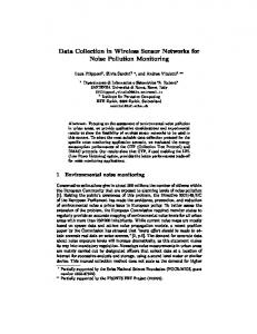
B. System Performance To compare with ADPEC, we fixed both transmission range (r) and h0 (see Section IV-A) as characteristic distance(dchar ) [9]. The whole network lifetime is divided into rounds with 100 time-frames each. That is, MAs relocate themselves every 100 iterations of data collection,to alleviate the “funneling effect”. The effect of balancing energy consumption with different moving strategies is verified first. We conduct the experiments under a stochastic topology and set CDPR as routing algorithm. Figure 6 shows the residual energy distribution of sensor with ADPEC and LADPEC respectively after 0, 100, 200, 300 rounds of data collecting. From the figure, we can see that 2 percent of nodes have almost depletes 20 percent of total energy after first round. The advantage is obvious after 200 rounds of data collection. The number of energy-rich nodes in LADPEC is nearly 3 times than that in ADPEC, which proves that LADPEC is more energy-balanced than ADPEC. To evaluate the elongation of network lifetime, we compare ADPEC, LADPEC with PERI [8] in which each MA sets it position along with the periphery of Voronoi cell. The simulation results in Figure 7 show that the © 2010 ACADEMY PUBLISHER

0

100

200

300

Time(# Rounds)

(b) LADPEC Figure 6. Residual energy distribution of alive sensors in given topology

network lifetime with LADPEC is almost 200% than that of ADPEC and PERI under both CDPR and LBSPR when half of nodes keep alive. Note that, ADPEC seems more efficient after 90% of sensors are dead as shown in Figure 7(a). As described in [9], the potential field exerted to MAs in ADPEC is from whole network. Therefore, MAs will keep stable when most of sensors are dead. However, the network coverage at the time is incomplete. In the above experiments, we assume a random network model with uniform distribution. Next, we compare the energy efficiency of those schemes in differing network distribution. In particular, a partial model where the sensors density in one half of circular area is higher than that of the other part is considered. The energy efficiency here is defined as the average consumed energy per round in the whole network. Figure 8 show the experimental results. It shows that LBSPR outperform CDPR in either of distribution. Moreover, we can see that the joint of LADPEC and LBSPR is the most energyefficient schemes among different composition. Notice that, both PERI and LADPEC perform better in partial distribution, since they are executed in a distributed way. C. Impact of Scalability In this part, we assess the scalability of the proposed schemes. That is, how the number of mobile aggregators or sensors influences the efficiency of whole network. To perform the simulation, we first distribute 500 sensors

1200 1000 800 600 400 PE

200 0

RI

AD

PEC PEC

LAD

1%

50%

P

90%

100%

Energy Efficiency(Consumed Energy/Rounds)

JOURNAL OF COMMUNICATIONS, VOL. 5, NO. 9, OCTOBER 2010

Network Lifetime (Number of Rounds)

672

CDPR LBSPR 0.020

0.015

0.010

0.005

0.000 PERI

ercentage of Node Death

ADPEC

LADPEC

Deployment Algorithm

(a) CDPR

(a) Network with uniform distribution

1200 1000 800 600 400 200

PE

RI

0

PEC PEC 100%

AD

LAD

1%

P

50%

90%

Energy Efficiency(Consumed Energy/Rounds)

Network Lifetime (Number of Rounds)

1400 0.055

CDPR 0.050

LBSPR

0.045

0.040

0.035

0.030

0.025

0.020

0.015

0.010

0.005

0.000 PERI

ercentage of Node Death

ADPEC

LADPEC

Deployment Algorithm

(b) Network with partial distribution

Figure 7. Network lifetime with different routing algorithms

Figure 8. Energy efficiency with different schemes under various nodes distribution

randomly in a circular field with radius 100 meters but vary the number of MAs from 5 to 100 with increment 10. The network lifetime is defined as the period of data collection until 90% sensors have depleted their energy. As seen in Figure 9, the energy efficiency increases with the number of MAs under both CDPR and LBSPR. However, the number of MAs up a certain threshold does not affect the energy efficiency. It can be explained that, the lifetime of the network increases with the number of MAs until each sensor can transmit the data in one or few hops to their affiliated aggregators. More MAs have no advantage and do not improve the energy efficiency. Next, we study the temporal efficiency. Given that MAs move in an ideal speed, we depict time efficiency as total execution time of deployment algorithms. Obviously, the execution depends on the experimental conditions. Here, all simulations run in the same duo-core laptop with 2GHz CPU and 2GB memory. Figure10 shows the calculated delay in seconds with different network size. The deployment delay keeps stable in LADPEC irrespective of network scale. On the contrary, ADPEC is a centralized protocol, thus the deployment delay is increased with the number of sensors and MAs. VI. C ONCLUSION In this paper, we study data collection problem with multiple aggregators for energy conservation in heterogeneous sensor networks. In particular, we propose a © 2010 ACADEMY PUBLISHER

Energy Efficiency(Consumed Energy/Rounds)

(b) LBSPR

CDPR

1.6

LBSPR 1.4

1.2

1.0

0.8

0.6

0.4

0

25

50

75

100

125

The Number of Mobile Aggregators(MAs)

Figure 9. Energy efficiency with different schemes

mobility-assisted hierarchy which addresses the joint effect of deployment protocols and routing algorithms. The extensive simulation results prove that mobility can increase energy efficiency of sensors and then prolong network lifetime. The findings also show that it might be appropriate to increase the number of MAs to improve the scalability. In the future research, we intent to discuss the real moving pattern of mobile elements. Also, we will continue to implement the proposed protocol in real network environment.

JOURNAL OF COMMUNICATIONS, VOL. 5, NO. 9, OCTOBER 2010

16

10) 10) ADPEC(# of MAs =50) LADPEC(# of MAs =50) ADPEC(# of MAs =

LADPEC(# of MAs =

Total deployment delay(seconds)

14 12 10 8 6 4 2 0 500

700

900

1100

1300

1500

The number of sensors

Figure 10. Temporal efficiency with different schemes

R EFERENCES [1] S. Tilak, N. B. Abu-Ghazaleh, and W. Heinzelman, “A taxonomy of wireless micro-sensor network models,” ACM Mobile Computing and Communications Review, vol. 6, pp. 28–37, Aug. 2002. [2] K. Akkaya and M. Younis, “A survey on routing protocols for wireless sensor networks,” Ad Hoc Network Journal, vol. 3, pp. 325–349, 2005. [3] W. B. Heinzelman, A. P. Chandrakasan, and H. Balakrishnan, “An application-specific protocol architecture for wireless microsensor networks,” IEEE Transactions On Wireless Communications, vol. 1, pp. 660–670, Oct. 2002. [4] S. Lindsey, C. Raghavendra, and K. M. Sivalingam, “Data gathering algorithms in sensor networks using energy metrics,” IEEE Transactions On Parallel and Distributed Systems, vol. 13, no. 9, Sep. 2002. [5] V. Mhatre and C. Rosenberg, “Design guidelines for wireless sensor networks: Communication, clustering and aggregation,” Ad Hoc Networks, 2004. [6] Y. P. Chen, A. L. Liestman, and J. Liu, “Energy-efficient data aggregation hierarchy for wireless sensor networks,” in Proceedings of the 2nd International Conference On Quality of Service in Heterogeneous Wired/Wireless Networks (QShine’05), 2005. [7] S. Bandyopadhyay and E. J. Coyle, “An energy efficient hierarchical clustering algorithm for wireless sensor networks,” in Proceedings of INFOCOM, 2003, pp. 1713– 1723. [8] J. Luo and J.-P. Hubaux, “Joint mobility and routing for lifetime elongation in wireless sensor networks,” in Proc. of INFOCOM, March 2005, pp. 1735–1746. [9] Z. Fan, Y. P. Chen, and H. Zhou, “An aggregator deployment protocol for energy conservation in wireless sensor networks,” in Proc. of IEEE International Conference Networking, Sensing and Control (ICNSC), Apr. 2008, pp. 1019–1024. [10] I. F. Akyildiz and I. H. Kasimoglu, “Wireless sensor and actor networks: Research challenges,” Ad Hoc Networks, vol. 2, pp. 351–367, 2004. [11] E. Ekic, Y. Gu, and D. Bozdag, “Mobility-based communication in wireless sensor networks,” IEEE Communications Magazine, vol. 44, pp. 56–62, 2006. [12] Y. Gu, D. Bozdag, R. W. Brewer, and E. Ekici, “Data harvesting with mobile elements in wireless sensor networks,” Computer Networks, vol. 50, pp. 3449–3465, 2006. [13] D. Jea, A. Somasundara, and M. Srivastava, “Multiple controlled mobile elements (data mules) for data collection in sensor networks,” in Proc. of the 1st International Conference on Distributed Computing in Sensor Systems (DCOSS), California, USA, Jun.-Jul. 2005, pp. 244–258.

© 2010 ACADEMY PUBLISHER

673

[14] Z. M. Wang, S. Basagni, E. Melachrinoudis, and C. Petrioli, “Exploiting sink mobility for maximizing sensor networks lifetime,” in Proc. of the 38th Hawaii International Conference on System Sciences, Jan. 2005, pp. 1–9. [15] S. R. Gandham, M. Dawande, R. Prakash, and S. Venkatesan, “Energy efficient schemes for wireless sensor networks with multiple mobile base stations,” in Proc. of GLOBECOM, 2003, pp. 377–381. [16] T. Melodia, D. Pompili, V. C. Gungor, and I. F. Akyildiz, “Communication and coordination in wireless sensor and actor networks,” IEEE Transactions On Mobile Computing, vol. 6, Oct. 2007. [17] I. F. Akyildiz, W. Su, Y. Sankarasubramaniam, and E. Cayirci, “A survey on sensor networks,” IEEE Communications Magazine, vol. 40, pp. 102–114, Aug. 2002. [18] R. C. Shah, S. Roy, S. Jain, and W. Brunette, “Data mules: Modeling a three-tier architecture for sparse sensor networks,” in Proc. of the 1st International Workshop on Sensor Network Protocols and Applications, May 2003, pp. 30–41. [19] A. Chakrabarti, A. Sabharwal, and B. Aazhang, “Using predictable observer mobility for power efficient design of sensor networks,” in Proc. of Information Processing in Sensor Networks (IPSN), 2003, pp. 129–145. [20] A. A. Somasundara, A. Ramamoorthy, and M. B. Srivastava, “Mobile element scheduling for efficient data collection in wireless sensor networks with dynamic deadlines,” in Proc. of the 25th IEEE International Real-Time Systems Symposium (RTSS), Dec. 2004, pp. 296–305. [21] J. Ma, C. Chen, and J. P. SALOMAA, “mwsn for large scale mobile sensing,” Journal of Signal Processing Systems, 2008. [22] R. W. Pazzi and A. Boukerche, “Mobile data collector strategy for delay-sensitive applications over wireless sensor networks,” Computer Communications, 2008. [23] J. Gao and L. Zhang, “Load-balanced short-path routing in wireless networks,” IEEE Transactions On parallel and Distributed Systems, Apr. 2006. [24] M. Bhardwaj, T. Garnett, and A. Chandrakasan, “Upper bounds on the lifetime of sensor networks,” in Proc. of ICC, Helsinki,Finland, Mar. 2001, pp. 785–790. [25] G. Wang, G. Cao, and T. L. Porta, “Movementassisted sensor deployment,” in Proc. of INFOCOM, Hongkong,China, Mar. 2004, pp. 2469–2479. [26] “Network simulator 2,” http://www.isi.edu/nsnam/ns/. [27] W. B. Heinzelman, “Application-specific protocol architectures for wireless networks,” Ph.D. dissertation, Massachusetts Institute of Technology, 2000. ZUZHI FAN received his Ph.D. degree in Computer science from Wuhan University, China in 2008. He is currently a lecturer in the college of information science&technology at Jinan University,China. His main research interests include wireless sensor network, mobile ad hoc computing and system security. The research activities have been supported by ”the Fundamental Research Funds for the Central Universities”, China. YUANZHU PETER CHEN is an assistant prof. in the Department of Computer Science at Memorial University of Newfoundland, St. John’s, Canada. He received his Ph.D. from Simon Fraser University in 2004 and B.Sc. from Peking University in 1999. Between 2004 and 2005 he was a postdoctoral researcher at Simon Fraser University. His research interests include mobile ad hoc networking, wireless sensor networking, distributed computing, combinatorial optimization, and graph theory.