Within such a curve, there will arise a bend or knee in the ...... Air Force Research Laboratory, http://www.vs.afrl.af.mil/Factsheets/shroud.html, Jan. 1998. Ayers ...
Modal and Impedance Modeling of a Conical Bore for Control Applications by
Kevin Farinholt
Thesis submitted to the Faculty of the Virginia Polytechnic Institute and State University in partial ful¯llment of the requirements for the degree of
Master of Science in
Mechanical Engineering
Donald J. Leo, Chair Daniel J. Inman Harry H. Robertshaw
October 2001 Blacksburg, Virginia Keywords: ppf control, conic sections, noise reduction, payload fairing Copyright by Kevin M. Farinholt, 2001
Modal and Impedance Modeling of a Conical Bore for Control Applications
Approved by Advising Committee:
In memory of my mother, Linda M. Farinholt
Abstract The research presented in this thesis focuses on the use of feedback control for lowering acoustic levels within launch vehicle payload fairings. Due to the predominance of conical geometries within payload fairings, our work focused on the analytical modeling of conical shrouds using modal and impedance based models. Incorporating an actuating boundary condition within a sealed enclosure, resonant frequencies and mode shapes were developed as functions of geometric and mechanical parameters of the enclosure and the actuator. Using a set of modal approximations, a set of matrix equations have been developed describing the homogeneous form of the wave equation. Extending to impedance techniques, the resonant frequencies of the structure were again calculated, providing analytical validation of each model. Expanding this impedance model to ¯rst order form, the acoustic model has been coupled with actuator dynamics yielding a complete model of the system relating pressure to control voltage. Using this coupled state-space model, control design using Linear Quadratic Regulator and Positive Position Feedback techniques has also been presented. Using the properties of LQR analysis, an analytical study into the degree of coupling between actuator and cavity as a function of actuator resonance has been conducted. Constructing an experimetnal test-bed for model validation and control implementation, a small sealed enclosure was built and out¯tted with sensors. Placing a control speaker at the small end of the cone the large opening was sealed with a rigid termination. An internal acoustic source was used to excite the system and pressure measurements were captured using an array of microphones located throughout the conic section. Using the parameters of this experimental test-bed, comparisons were made between LQR and PPF control designs. Using an impulse disturbance to excite the system, LQR simulations predicted reductions of 53.2% below those of the PPF design, while the control voltages corresponding to these reductions were 43.8% higher for
iv
LQR control. Actual application of these control designs showed that the ability to manually set PPF gains made this design technique much more convenient for actual implementation. Yielding overall attenuation of 38% with control voltages below 200 mV, single-channel low authority control was seen to be an e®ective solution for low frequency noise reduction. Control was then expanded to a larger geometry representative of Minotaur fairings. Designing strictly from experimental results, overall reductions of 38.5% were observed. Requiring slightly larger control voltages than those of the conical cavity, peak voltages were still found to be less than 306 mV. Extrapolating to higher excitation levels of 140 dB, overall power requirements for 38.5% pressure reductions were estimated to be less than 16 W.
v
Acknowledgments First I would like to extend my thanks to my advisor, Dr. Donald J. Leo for his encouragement and advice throughout my graduate studies. Special thanks also go to Dr. Daniel Inman for his insight into controllability and orthogonality issues investigated in this research. I would also like to thank Dr. Harry Robertshaw and Dr. William Saunders for their input and experience related to this research. I would especially like to thank my parents for their continued support and love throughout my life and education, and it is to my mother that this work is dedicated. I would also like to thank my brother, sisters and all my friends for their understanding, humor and help over the last year. This research has been supported by the Air Force Research Laboratory at Kirtland Air Force base in Albuquerque, NM and was administered by Syndetix, Inc. under purchase order 00-04-6838. I would also like to thank Dr. Steven Lane of AFRL who has overseen this research.
vi
Contents List of Tables
x
List of Figures
xi
Nomenclature
xiv
Chapter 1 Introduction
1
1.1
Motivation
. . . . . . . . . . . . . . . . . . . . . . . . . . . . . . . . . . . .
1
1.2
History of Acoustics . . . . . . . . . . . . . . . . . . . . . . . . . . . . . . .
2
1.3
Literature Review
. . . . . . . . . . . . . . . . . . . . . . . . . . . . . . . .
4
1.3.1
Studies Associated with Payload Fairings . . . . . . . . . . . . . . .
4
1.3.2
Previous Acoustic Models . . . . . . . . . . . . . . . . . . . . . . . .
5
1.3.3
Con°icting Developments in Literature on Spherical Waves . . . . .
7
1.3.4
Control for Active Noise Reduction . . . . . . . . . . . . . . . . . . .
8
Thesis Overview . . . . . . . . . . . . . . . . . . . . . . . . . . . . . . . . .
9
1.4.1
Contribution . . . . . . . . . . . . . . . . . . . . . . . . . . . . . . .
9
1.4.2
Approach . . . . . . . . . . . . . . . . . . . . . . . . . . . . . . . . .
10
1.4
Chapter 2 Modal Model of a Conical Bore 2.1
2.2
12
Conservation of Mass and Momentum . . . . . . . . . . . . . . . . . . . . .
12
2.1.1
Conservation of Mass . . . . . . . . . . . . . . . . . . . . . . . . . .
13
2.1.2
Conservation of Momentum . . . . . . . . . . . . . . . . . . . . . . .
14
2.1.3
The Wave Equation . . . . . . . . . . . . . . . . . . . . . . . . . . .
14
De¯ning the Wave Equation using Acoustic Potential . . . . . . . . . . . . .
15
2.2.1
Solving for the Acoustic Potential . . . . . . . . . . . . . . . . . . .
16
2.2.2
Extension to particle acceleration and displacement . . . . . . . . .
17
vii
2.2.3
Separation of variables . . . . . . . . . . . . . . . . . . . . . . . . . .
18
Boundary Value Problem in a Conical Bore . . . . . . . . . . . . . . . . . .
19
2.3.1
De¯nition of boundary conditions . . . . . . . . . . . . . . . . . . . .
19
2.3.2
Implementation of boundary conditions . . . . . . . . . . . . . . . .
21
2.3.3
Acoustic mode shapes . . . . . . . . . . . . . . . . . . . . . . . . . .
23
2.4
Equation of Motion for Unforced System . . . . . . . . . . . . . . . . . . . .
25
2.5
Analytical Validation of the Modal Model . . . . . . . . . . . . . . . . . . .
26
2.6
Chapter Summary . . . . . . . . . . . . . . . . . . . . . . . . . . . . . . . .
28
2.3
Chapter 3 Impedance Model of a Conical Bore
29
3.1
Electrical equivalent to acoustic system . . . . . . . . . . . . . . . . . . . .
29
3.2
Model development . . . . . . . . . . . . . . . . . . . . . . . . . . . . . . . .
32
3.2.1
Speaker Equations . . . . . . . . . . . . . . . . . . . . . . . . . . . .
32
3.2.2
Cavity Equations . . . . . . . . . . . . . . . . . . . . . . . . . . . . .
35
3.3
Coupled State-Space Model . . . . . . . . . . . . . . . . . . . . . . . . . . .
37
3.4
Application to a Sample Geometry . . . . . . . . . . . . . . . . . . . . . . .
37
3.4.1
space representations . . . . . . . . . . . . . . . . . . . . . . . . . . .
38
Comparison of Modal and Impedance Predictions . . . . . . . . . . .
39
Chapter Summary . . . . . . . . . . . . . . . . . . . . . . . . . . . . . . . .
40
3.4.2 3.5
Comparison of cavity models: frequency-domain, s-plane and state-
Chapter 4 Control Design 4.1
42
Design of a Linear Quadratic Regulator . . . . . . . . . . . . . . . . . . . .
43
4.1.1
LQR controller design . . . . . . . . . . . . . . . . . . . . . . . . . .
43
4.1.2
Optimization and Simulation of LQR
. . . . . . . . . . . . . . . . .
44
Design using Positive Position Feedback . . . . . . . . . . . . . . . . . . . .
50
4.2.1
PPF controller design . . . . . . . . . . . . . . . . . . . . . . . . . .
51
4.2.2
Simulation of PPF . . . . . . . . . . . . . . . . . . . . . . . . . . . .
52
4.3
Comparison of LQR and PPF Simulations . . . . . . . . . . . . . . . . . . .
53
4.4
Chapter Summary . . . . . . . . . . . . . . . . . . . . . . . . . . . . . . . .
55
4.2
Chapter 5 Experimental Veri¯cation 5.1
57
Experimental Setup . . . . . . . . . . . . . . . . . . . . . . . . . . . . . . .
viii
57
5.2
Validation of Modal and Impedance-Based Models . . . . . . . . . . . . . .
60
5.2.1
Modal model . . . . . . . . . . . . . . . . . . . . . . . . . . . . . . .
60
5.2.2
Impedance-based model . . . . . . . . . . . . . . . . . . . . . . . . .
62
5.3
Control of the Conical Bore . . . . . . . . . . . . . . . . . . . . . . . . . . .
64
5.4
PPF Control Applied to the Full Fairing Geometry . . . . . . . . . . . . . .
72
5.5
Chapter Summary . . . . . . . . . . . . . . . . . . . . . . . . . . . . . . . .
77
Chapter 6 Conclusions
78
6.1
Contribution . . . . . . . . . . . . . . . . . . . . . . . . . . . . . . . . . . .
78
6.2
Conclusions of our Investigation . . . . . . . . . . . . . . . . . . . . . . . . .
79
6.3
Recommendations for Future Work . . . . . . . . . . . . . . . . . . . . . . .
81
Bibliography
83
Appendix A Non-orthogonality and its Impact on Self-Adjointness and the Symmetry of State Matrix
87
Appendix B Development of a Generalized Forcing Function
90
Appendix C Mathematica Code Using Modal Approximation Methods
95
Appendix D Mathematica Code Using Impedance Methods
105
Appendix E MATLAB Program Used to Generate LQR Curves
112
Appendix F MATLAB Program to generate LQR and PPF controllers
118
Vita
130
ix
List of Tables 2.1
Geometric, electrical and mechanical parameters of the experimental set-up. These values are used for analytical models. . . . . . . . . . . . . . . . . . .
2.2
Comparison of actuation model with models developed by Ayers et al. (all values in Hz). . . . . . . . . . . . . . . . . . . . . . . . . . . . . . . . . . . .
3.1
25
27
Comparison of resonance frequencies from modal and impedance based models(all values in Hz). . . . . . . . . . . . . . . . . . . . . . . . . . . . . . . .
40
4.1
Design parameters of the PPF compensator . . . . . . . . . . . . . . . . . .
54
5.1
Comparison of the resonance frequencies of our modal model with those of an experimental test stand for rigid-rigid and actuating-rigid boundary conditions (all frequencies in Hz). . . . . . . . . . . . . . . . . . . . . . . . .
5.2
61
Comparison of the resonance frequencies of our impedance-based model with those of an experimental test stand for rigid-rigid and actuating-rigid boundary conditions (all frequencies in Hz). . . . . . . . . . . . . . . . . . . . . .
62
5.3
Comparison of experimental and state-space model results (all values in Hz).
64
5.4
Design parameters of the PPF compensator . . . . . . . . . . . . . . . . . .
67
5.5
Pressure reductions in the conical bore test stand. . . . . . . . . . . . . . .
71
5.6
Pressure reductions in the full fairing geometry . . . . . . . . . . . . . . . .
76
x
List of Figures 1.1
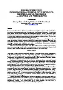
Various shroud geometries: a.) grid sti®ened USAF launch vehicle payload fairing, b.) Titan IV payload fairing by Lockheed Martin and c.) Delta II payload fairing by Boeing during launch. . . . . . . . . . . . . . . . . . . . .
1.2
3
Drawing from Principia (1686) by Sir Isaac Newton. Illustrates sound propagating through an ori¯ce, which was "Adapted from Sir Isaac Newton's Principia, 4th ed., 1726, reprinted 1871, by MacLehose, Glasgow, p. 359", from Pierce (1991) p. 5 . . . . . . . . . . . . . . . . . . . . . . . . . . . . .
4
1.3
Discontinuities with narrowing or terminating geometries. . . . . . . . . . .
8
2.1
Compression of a °uid within a conical bore. a.) Compression from a driver operating with velocity u over time t. b.) Control volume of °uid, p; ½; u at a location, r, and p; ½; u at displaced location r + dr. . . . . . . . . . . . . .
13
2.2
The spherical contour of the actuator face. . . . . . . . . . . . . . . . . . . .
16
2.3
Parameters used to de¯ne a conical bore having reactive-rigid boundary conditions . . . . . . . . . . . . . . . . . . . . . . . . . . . . . . . . . . . . . . .
2.4
19
Transcendental relationship for natural frequencies of an actuating-closed conical bore . . . . . . . . . . . . . . . . . . . . . . . . . . . . . . . . . . . .
23
2.5
First three acoustic modes for actuating-closed conical bore. . . . . . . . . .
24
3.1
Transducer model of speaker and cavity system. . . . . . . . . . . . . . . . .
30
3.2
Electric circuit of a permanent magnet speaker . . . . . . . . . . . . . . . .
33
3.3
Spring-mass-damper system subjected to an applied force Bli and applied pressure p. . . . . . . . . . . . . . . . . . . . . . . . . . . . . . . . . . . . . .
3.4
34
Comparison of impedance (solid), s-plane (dashed) and state-space (dotted) models. . . . . . . . . . . . . . . . . . . . . . . . . . . . . . . . . . . . . . . xi
38
3.5
Open-loop frequency response of the fully coupled system. . . . . . . . . . .
39
4.1
Trade-o® curve from Linear Quadratic Regulator design. . . . . . . . . . . .
45
4.2
RMS pressure versus RMS control voltage for multiple actuator resonances, each as a function of Q2 . . . . . . . . . . . . . . . . . . . . . . . . . . . . . .
46
4.3
RMS pressure versus RMS control voltage, each as a function of Q2 . . . . .
47
4.4
Impulse response (Q2 = 122). a.) Open versus closed-loop pressure response b.) Control voltage
4.5
48
Impulse response (Q2 = 3500). a.) Open versus closed-loop pressure response b.) Control voltage
4.6
. . . . . . . . . . . . . . . . . . . . . . . . . . . . . . .
. . . . . . . . . . . . . . . . . . . . . . . . . . . . . . .
49
Frequency response of the open-loop system having an LQR based compensator (Q2 = 3500). . . . . . . . . . . . . . . . . . . . . . . . . . . . . . . . .
50
4.7
Three mode PPF controller. . . . . . . . . . . . . . . . . . . . . . . . . . . .
52
4.8
Impulse response with PPF ¯lter. a.) Open versus closed-loop pressure response b.) Control voltage
4.9
. . . . . . . . . . . . . . . . . . . . . . . . . .
53
Comparison of closed-loop performance between LQR and PPF compensators given an impulse excitation. a.) Pressure response b.) Control voltage . . .
55
4.10 Comparison of operating points of LQR and PPF simulations. . . . . . . . .
56
5.1
Experimental setup for conical bore validation and control. a.) rigid-rigid boundary conditions, b.) actuating-rigid boundary conditions . . . . . . . .
58
5.2
Block diagram illustrating the experimental set-up.
59
5.3
Experimentally obtained resonances for rigid-rigid and actuating-rigid bound-
. . . . . . . . . . . . .
ary conditions. . . . . . . . . . . . . . . . . . . . . . . . . . . . . . . . . . . 5.4
Open-loop comparison of experimentally obtained frequency response with that predicted by the impedance based model. . . . . . . . . . . . . . . . .
5.5
63
SIMULINK diagram of PPF compensator used by dSPACE to implement feedback control on the experimental test stand. . . . . . . . . . . . . . . .
5.6
60
65
Open (dashed) versus closed (solid) performance for collocated sensor-actuator pair with PPF parameters of Table 4.1. This frequency response relates output pressure to disturbance signal. . . . . . . . . . . . . . . . . . . . . . . .
xii
66
5.7
Global comparison of open-loop (dashed) and closed-loop (solid) performance with gain PPF parameters of Table 4.1. Frequency response throughout the conical bore relating output pressure to the disturbance signal: microphone at
(r2 ¡r1 ) 4
(top-left), microphone at
(r2 ¡r1 ) 2
(top-right), microphone at
3(r2 ¡r1 ) 4
(bottom-left) and microphone at r2 (bottom-right). . . . . . . . . . . . . . . 5.8
68
Open-loop (dashed) versus closed-loop (solid) performance for collocated sensor-actuator pair with PPF parameters of Table 5.4. This frequency re-
5.9
sponse relates output pressure to disturbance signal. . . . . . . . . . . . . .
69
Required control voltage for PPF compensator of Table 5.4. . . . . . . . . .
69
5.10 Global comparison of open (dashed) and closed (solid) loop performance with gain PPF parameters of Table 5.4. Frequency response throughout the conical bore relating pressure to disturbance: microphone at left), microphone at
(r2 ¡r1 ) 2
(top-right), microphone at
and microphone at r2 (bottom-right).
3(r2 ¡r1 ) 4
(r2 ¡r1 ) 4
(top-
(bottom-left)
. . . . . . . . . . . . . . . . . . . . .
70
5.11 Geometric parameters of the Lexan payload fairing. . . . . . . . . . . . . .
72
5.12 Open-loop transfer function of the Lexan fairing. . . . . . . . . . . . . . . .
73
5.13 Open versus closed loop performance within the fairing for collocated microphone. This frequency response relates output pressure to disturbance signal. . . . . . . . . . . . . . . . . . . . . . . . . . . . . . . . . . . . . . . .
74
5.14 Global comparison of open (dashed) and closed (solid) loop performance within the fairing model. Each frequency response relates output pressure to disturbance signal. . . . . . . . . . . . . . . . . . . . . . . . . . . . . . . . .
75
5.15 Required control voltage for PPF compensator of Table 5.6. . . . . . . . . .
76
A.1 First three acoustic modes for actuating-closed conical bore. . . . . . . . . .
88
F.1 SIMULINKdiagram of the system using LQR compensation . . . . . . . . . . .
126
F.2 SIMULINKdiagram of the system using PPF compensation . . . . . . . . . . .
127
xiii
Nomenclature
r - spatial coordinate, de¯ned as distance from cone apex t - time r1 - distance from cone apex to the small opening of the conic section r2 - distance from cone apex to the large opening of the conic section ½tot (r; t) - total density of a °uid particle ½o - ambient density of a °uid particle ½(r; t - acoustic or instantaneous density of a °uid particle u(r; t) - particle velocity x(r; t) - particle displacement u_ - particle acceleration ptot (r; t) - total pressure po - ambient pressure p(r; t) - acoustic pressure co - speed of sound S(r) - cross-sectional area at location r µ - angle of divergence of cone Á(r; t) - acoustic potential function f (ct ¨ r) - solution to the plane wave equation '(r) - spatial component of acoustic potential ´(t) - temporal component of acoustic potential ¯(t) - the integral of ´(t) £ ¤ ! - frequency rad s ma - mass of actuator
xiv
ka - mechanical sti®ness of actuator ca - mechanical damping of actuator F (t) - external forcing function S(r1 ) - cross sectional area at r1 , also the actuator area p j - ¡1 - the imaginary varible k - wave number A; B - amplitude coe±cients of acoustic potential M - mass matrix K - sti®ness matrix fA - frequency of Ayers et al. model in [Hz] fAo - fundamental frequency of Ayers et al. model vin (t) - input voltage i(t) - current U (r; t) - volume velocity e(t) - electromotive voltage ze - electrical impedance zm - mechanical impedance za - acoustic impedance f - force induced by speaker coil f1 - mechanical force of speaker f2 - force generated by pressure at r1 Bl - electromotive constant or °ux R - electrical resistance of actuator L - electrical inductance of actuator s - Laplace variable P (s) - pressure in s-domain U (s) - volume velocity in s-domain !z - frequency locations of acoustic zeros !p - frequency locations of acoustic poles qc - states of the acoustic cavity
£ rad ¤ s
£ rad ¤ s
qa - states of the acutator Ac ; Bc ; Cc - state space matrices of cavity xv
Aa ; Bav ; Bap ; Ca - state space matrices of speaker F; G; H; J - state space matrices of coupled system q(t) - state variables v(t) - input control voltage Q1 - state weighting matrix Q2 - control e®ort weighting matrix Fcl ; Gcl ; Hcl ; Jcl - state space matrices of closed loop system Klqr - LQR feedback gain Lest - estimator gain Fcomp ; Gcomp ; Hcomp ; Jcomp - state space matrices of the LQR compensator » - system variable for PPF derivation ´ - compensator variable for PPF derivation ³f - compensator damping ratio for PPF ¯lter !f - compensator frequency for PPF ¯lter g - PPF gain fl - Lower frequency limit for mean squared pressure calculations fh - High frequency limit for mean squared pressure calculations
xvi
Chapter 1
Introduction 1.1
Motivation
Throughout its operational lifetime, the most strenuous loads that a satellite system will be subjected to are experienced during just the ¯rst few minutes of launch, Glaese (1999) and Leo (1998). Air°ow along the outer walls of payload fairings, coupled with vibrations transmitted from booster rockets induce acoustic resonances within the shroud which houses satellite components. Reaching levels of 120 to 150 dB, Green (2000), damage to instrumentation is a very real concern for designers of satellite systems. Current methods for addressing these concerns primarily consist of the over design of satellite components themselves. Building stronger satellites ensures that they will survive launch, however, at the expense of both functional e±ciency as well as cost. With deployment costs estimated at $10,000 to $12,000 per pound according to the Federation of American Scientists FAS (1997), the necessity to over design satellite components carries with it a high monetary cost. In conjunction with the desire to reduce payload mass, rocket designers have begun the construction of new, lighter weight launch vehicle payload fairings. Moving to sti®ened composite materials, up to 61% reductions in fairing weight have been obtained according to the Space Vehicles Directorate of the Air Force Research Laboratory AFRL (1998). While such advancements have reduced launch costs, they have adversely a®ected the acoustic environment within the fairing. Reductions in weight lower excitation energies, thus increasing both structural vibrations and their coupled a®ect on acoustic resonances within the shroud. To combat these issues, installation of acoustic blankets have been used 1
along the inner walls of fairings. Dissipating acoustic energy as heat, these methods have proven successful in targeting higher frequency resonances. However, the e®ectiveness of these materials is directly related to the ratio of material thickness to acoustic wavelength, requiring greater thicknesses for longer wavelengths. Thus, there is a limit at which the required thickness associated with lower frequencies infringes upon the available volume within the fairing. With the typical installation of blankets between 2 and 4 inches thick, passive attenuation is limited to frequencies above 300 to 400 Hz for these materials. While other passive techniques can address low frequency attenuation the volume requirements of both Helmholtz resonators and passive absorbers impede their application. However, the incorporation of active techniques for either tuning absorbers or actively canceling sound o®er possible and practical means of reducing noise levels. To properly implement active control on any system, an understanding of the dynamics within that system should be understood. Considering the various geometries of existing payload fairings, shown in Figure 1.1, one common attribute is the presence of conical and/or cylindrical cavities. Analytical solutions to wave propagation within cylindrical enclosures have been well studied. However, investigations into conical bores have been limited mostly to musical applications. Because of the limited research into these geometries, especially for control applications, the research presented in this thesis includes developments of both modal and impedance models for the purpose of control implementation.
1.2
History of Acoustics
People have theorized that sound propagates as waves for over 2500 years. With its birth in the philosophical community during the times of Pythagoras ( 550 B.C.) and Aristotle ( 384-322 B.C.), it was not until the seventeenth century that experimental ¯ndings related sound propagation to source vibration. In 1636, Marin Mersenne published his ¯ndings in Harmonie universelle relating the vibration of two strings, oscillating one octave apart, with the frequency of their respective tones. This combined with work by Galileo Galilei provided the ¯rst collection of experimental proof that sound and source frequencies must be the same. Incidentally, at the same time as the work by Mersenne and Galilei, other researchers were proposing alternate explanations of sound propagation. Using ray theory, Gassendi
2
Figure 1.1: Various shroud geometries: a.) grid sti®ened USAF launch vehicle payload fairing, b.) Titan IV payload fairing by Lockheed Martin and c.) Delta II payload fairing by Boeing during launch. proposed that sound was due \to a stream of `atoms' emitted by the sounding body; velocity of sound is speed of atoms; frequency is number emitted per unit time." [Pierce (1991) p.4]. Arising at the same time as optical sciences, ray theory was later found to be a mathematical approximation of wave theory through work by Reynolds and Rayleigh in the nineteenth century. However, these ¯ndings by Reynolds and Rayleigh were based upon the mathematical development of wave theory, which began in the late seventeenth century with Sir Isaac Newton. Theorizing that acoustics propagate in wave patterns, Figure 1.2 illustrates Newton's conception of acoustic transmission through an ori¯ce. Continuing with advancements by Euler, Lagrange and d'Alembert, a structured view of acoustic wave theory was developed over the century following Newton's developments. With the wave equation's conception for general vibrations and sound, the basis for today's understanding of acoustics was laid. Building upon the principles of Newton, Euler, Lagrange and d'Alembert the ¯eld of acoustics was born, and it is these concepts which are applied in the modeling component of this thesis (Pierce, 1991).
3
Figure 1.2: Drawing from Principia (1686) by Sir Isaac Newton. Illustrates sound propagating through an ori¯ce, which was "Adapted from Sir Isaac Newton's Principia, 4th ed., 1726, reprinted 1871, by MacLehose, Glasgow, p. 359", from Pierce (1991) p. 5
1.3 1.3.1
Literature Review Studies Associated with Payload Fairings
The investigation into active noise reduction within payload fairings has been a topic of interest for many years, especially for agencies such as the Air Force Research Laboratory and the National Aeronautics and Space Administration (NASA). With external acoustic loads up to 150 dB (Glaese, 1999; Leo, 1998) much work has been conducted for active absorption or cancelation of sound. Himelblau (1992) of the Jet Propulsion Laboratory documents studies on the Titan IV payload fairing to establish the acoustic levels expected during the actual launch of the Cassini spacecraft. In this study, the Titan IV was out¯tted with 3 inch thick acoustic blankets along with an array of microphones corresponding to Cassini's expected location during launch. Four separate fairings were launched in this study with a collection of acoustical and °ight data for each launch. The outcome of this investigation was the statistical analysis of data describing the interior acoustic environment of the Titan IV during actual launch conditions. Other studies by engineers at CSA Engineering, Inc. have looked into the vibroacoustic modeling of launch vehicles for acoustic control. Leo (1998) presents work into
4
the structural and acoustic ¯nite element modeling of a payload fairing for the purpose of implementing localized feedback control. In this study, the authors demonstrate that control can be applied using proof-mass and piezoceramic actuators, and that reductions in acoustic levels are possible. Glaese (1999) later presents the simulated and experimental results of a similar study on the STARS payload fairing built by McDonnell Douglas. Using piezo strain sensors and piezo actuators, these authors found that it is possible to increase structural damping within the fairing using a single controller consisting of eight actuators. In addition to these studies, researchers at Duke University have investigated active control using spatially weighted arrays within acoustic enclosures, (Lane and Clark, 2000). Using a system of multiple collocated sensor-actuator pairs, measurements within the enclosure are taken, processed by the controller using H2 control laws, and implemented using a spatially weighted array. Experimentally tested in an aluminum aircraft fuselage supplied by Lord Corporation, 6 dB reductions in the global acoustic levels were achieved for a single-mode controller. Expanding to a ¯ve-mode controller, the authors found that multiple mode attenuation was also obtainable within the test structure. Along with the modeling and control of fairings, actuator design has proven to be a result of these studies. Developing a light weight actuator, Green (2000) achieved low frequency performance using piezoceramic actuation. Using cantilever con¯gurations, signi¯cant improvements were obtained when comparing noise to weight ratios with those of conventional permanent magnet actuators. However, limitations in stroke and overall power output impede its application presently. Additionally, work done by Henderson et al. (2001) investigates decreases in actuator volume while maintaining low frequency performance. Using an partially evacuated enclosure, the authors demonstrate that the depressurization of the speaker enclosure reduces the resonance frequency of the speaker. Thus, the actual volume of this enclosure could be reduced without increasing the operating frequency, provided that a suitable level of evacuation can be applied and maintained within the speaker enclosure.
1.3.2
Previous Acoustic Models
While many of the previous studies related to payload fairing have dealt with understanding the acoustic levels and resonances within the shroud, most modeling approaches have relied strictly on Finite Element models. Providing accurate representations of the enclosed 5
geometry one disadvantage of most Finite element packages is found in the size of the system matrices. In order to e®ectively apply control design and simulation based upon these models matrix reductions must be implemented, otherwise the analysis becomes computationally intensive. One way to avoid this complexity is the development of analytical models. Provided that the geometries are relatively simple with few discontinuities, analytical solutions can be obtained and implemented for the system. Previous work has been conducted with many basic geometries and it is upon this work that our research has been conducted. Cylindrical geometries have been studied throughout much of the history of the ¯eld of acoustics. Lending themselves to plane wave analysis, analytical models of tubes having open and closed boundary conditions can be obtained with relative ease. As the basic model for many Acoustics courses, the in¯nite ba²e has been used to describe one directional wave propagation in many textbooks, see Rayleigh (1877), Morse (1968), Bies (1996) or Kinsler (1997). Placing a rigid termination at one or both ends of the tube introduces two plane waves, one traveling in the positive direction with another traveling in the negative direction. Again, such solutions are common and relatively easy to reproduce. Introducing a resistive boundary condition complicates analysis slightly as the boundary dynamics must be coupled with the acoustic cavity Kinsler (1997). Kinsler and Frey (1997) present a detailed approach to such a problem in which they apply a driver at one location with a rigid boundary condition serving as the other termination. Using the mechanical impedance of the driver along with the acoustic impedance of a sealed tube, the authors generate a relationship between the input force of the driver to the pressure at each end of the cylinder. Similarly, Nelson and Elliot (1995) present an open piston in their development of an one-dimensional wave. Expanding upon this model, Nelson and Elliot consider both the presence of a monopole and a dipole source as the actuator, addressing actuators which maintain either pressure or particle velocity on each side of the piston. While each of these models couple actuator and acoustic dynamics, they address only cylindrical geometries. As a waveguide, cylinders provide a good basepoint for learning analysis techniques, explaining why they are widely used in texts. However, another waveguide which presents similar one-dimensional analysis techniques, but is not employed as readily in textbooks, is the conical bore. With fewer practical applications, conical 6
waveguides have received less attention in their development, especially for control applications. One area which has focused some attention on conical bores is the ¯eld of musical instruments. As the basic shape for several woodwind instruments, most modeling is for the purpose of understanding musical tones (Olson, 1967; Rigden, 1977; Taylor, 1992), to properly mimic such instruments electronically. Due to the geometry of a conical bore, assuming a spherical source at the apex of the cone, or one having a spherical contour associated with its radial distance from the apex, allows for spherically expanding waves to be used in the analysis. Ayers et al. (1985) develops the characteristic equation for conical bores having four separate con¯gurations of simple boundary conditions. Solving for open-open, open-closed, closed-open and closed-closed boundaries, the transcendental equations describing resonance frequencies are obtained, along with a visual representation of the standing waves.
1.3.3
Con°icting Developments in Literature on Spherical Waves
One issue in the development of these models is the reliance on physical intuition in the interpretation of results. Such a reliance o®ers room for incorrect conjectures, leading to some confusion in the interpretation of results. Ayers et al. (1985) write their article for the purpose of clarifying issues associated with the unusual behavior of waves near the apex of a conical cavity. With their review of preexisting literature addressing this topic, they found that over two thirds of the references provide incomplete or inaccurate conclusions relative to the behavior of truncated cones at their small end. Similarly, in a discussion of how sound waves behave in the presence of geometric discontinuities within conical bores, Gilbert (1989) critically disagrees with the ¯ndings of Agull¶ o (1992) concerning growing re°ections. With a narrowing of the cone, Figure 1.3, the propagating wave form is re°ected back onto itself at the discontinuity. Applying conventional analysis techniques, such re°ections should ultimately lead to an exponential growth in the sound, as stated by both Gilbert (1989) and Agull¶o (1992). The discrepancies of Agull¶o et al. are in their explanations of why this exponential growth doesn't occur physically. While such arguments are present, the correlation of results in this thesis compare model results derived from geometries with terminations normal to wave propagation and experimental results from a geometry similar to the terminated cone of Figure 1.3. The 7
Figure 1.3: Discontinuities with narrowing or terminating geometries. ¯ndings of this study indicate that the discrepancies debated in these articles are practically negligible in the physical system studied in this work.
1.3.4
Control for Active Noise Reduction
Most of today's approaches to active noise reduction rely upon feedforward control techniques. Feeding disturbance signals directly through the system compensator for acoustic control, one major assumption is that the disturbance is known and measurable. While this method of control design has bene¯ts over conventional feedback techniques, Saunders (1993), its reliance on knowing the disturbance makes it impractical for systems in which this disturbance path cannot be modeled. For such systems, feedback control remains the most viable option. While this method must deal with issues concerning reduced robustness and stability relative to feedforward techniques, it possesses the ability to address the transient performance of a system (Green, 2000). Providing direct information about the system performance, feedback methods use the present output of a dynamic system to alter and control the input signal through the use of a compensator. With a wide range of compensator designs ranging from frequency domain designs to pole placement methods, both classical and modern control techniques have been widely researched and implemented. One type of feedback control design which lends itself to active noise reduction along with other control applications is Linear Quadratic 8
Regulator design. As a standard control technique in state-space systems, the derivation and application can be found in many textbooks, Franklin (1998) and Friedland (1986). Allowing for the individual weighting of system response (Q) and control e®ort (R), LQR also gives the designer the opportunity to specify the importance of speci¯c modes relative to one another. Also in such designs, an optimal ratio of
Q R
can be obtained through the
development of a tradeo® curve between RMS values of the system response and control e®ort, each as functions of
Q R.
Within such a curve, there will arise a bend or knee in the
convexity of the trade o® curve, indicating the optimal ratio of these parameters (Boyd (1997); Leo (1995)). Alternately, the development of a controller using Positive Position Feedback can be used in active noise control. Providing the ability to target speci¯c modes, this technique gives the designer the ability to increase damping at desired resonance locations. McEver p (1999) found that the overestimation of these resonance frequencies, by a factor of 2, provides for optimal performance. Also, when targeting multiple modes, the gain speci¯cation for each individual PPF ¯lter must be selectively chosen as discussed by DeGuilio (2000). Due to interactions between high frequency gains and low frequency dynamics, the gains must be chosen in a top-down approach. As such, the ¯lter for the highest frequency mode must be designed ¯rst, working down through the modes until the lowest frequency ¯lter is designed. Altering from this technique introduces a higher probability of developing an unstable compensator through issues presented by DeGuilio (2000). One important advantage of this technique is that it can be implemented almost directly from experimental data. While many control techniques such as LQR require plant models, all that is really needed for PPF design are the system resonances, where ¯lter damping and gains can be determined iteratively in many applications.
1.4 1.4.1
Thesis Overview Contribution
The purpose of the research presented in this thesis is the attenuation of noise levels within launch vehicle payload fairings through the use of feedback control. Focusing on geometries similar to those found on typical sounding rockets, we have developed analytical models which predict resonance and modal properties of the acoustic environment. Having devel9
oped two separate models using modal approximation and impedance based techniques, a full characterization of the longitudinal waves within a conical bore having actuating and rigid boundary conditions has been accomplished. Allowing full variation in the mass, damping and sti®ness properties of a control actuator, ¯rst-order representation of the conical fairing have been generated. Analytical and experimental comparison was used to validate the model for multiple actuator parameters. Upon this model, investigations of Linear Quadratic Regulator and Positive Position Feedback techniques have been presented and discussed. Due to very small variations in open-loop and closed-loop pole locations for the LQR compensated system, PPF design was chosen and applied for simulation and experimental application. Implementing these controllers has shown that signi¯cant reductions in sound levels can be obtained using low authority control based on PPF design techniques. With RMS pressure reductions of 38.2% within the test-stand, power requirements were held to levels of 0.92 mW. Our study also worked to expand the control design to larger volumes with varying geometries. Selecting a fairing geometry of the Minotaur class, a half-scale model was constructed and PPF control was designed and applied. From this portion of our study the abilities of low authority control was again demonstrated as 38.5% reductions in RMS pressure were achieved. In this application power requirements were measured to be below 1.52 mW. Obtained for systems with disturbance levels of 100 dB (C-weight), the results of our study were extended to sound levels of 140 dB, correlating to those measured during actual launch conditions. Estimating power levels of 15.2 W for the half-scale model, the anticipated power requirements necessary to apply such control on a full scale fairing are on the order of 65 W, considering volumetric increases. In its entirety, the research that we have conducted has addressed the modeling and control of the fairings with conical geometries, ¯nding that control using single actuator-sensor pairing is both possible and e®ective in lowering noise levels within a sealed environment.
1.4.2
Approach
Modal modeling of the conical bore is presented in Chapter 2 with a further discussion of the asymmetry properties continued in Appendix A. Chapter 3 discusses the impedance model development and its coupling with actuator dynamics. Development of the statespace model used for simulation is also presented in Chapter 3, with a discussion of the actual controller designs found in Chapter 4. Experimental results for accuracy of each 10
model is presented in Chapter 5, along with the results from actual implementation of both LQR and PPF control on the conical fairing, and of PPF control on the full fairing shroud. Chapter 6 wraps up with the conclusions of this research along with recommendations for future work. Mathematical codes for model and compensator designs are found in the Appendices.
11
Chapter 2
Modal Model of a Conical Bore In most noise control applications the conventional method for approaching a problem begins with an impedance model of the system. However, for this research the ¯rst model development uses a modal approximation of a sealed conical bore having one rigid and one actuating boundary condition. Using conservation laws for mass and momentum a modal approximation of the system can be developed and an equation of motion extracted directly. Without instituting the steady state assumption both velocity and pressure variables can be maintained, allowing for analysis of the transient performance of the system. Developed directly from basic acoustic equations, the matrix form of an equation of motion can be developed that couples the electrical dynamics of the actuator with the acoustic system providing a full model of the system
2.1
Conservation of Mass and Momentum
Beginning with the driver system illustrated in Figure 2.1 two conservation laws must be upheld across the control volume, conservation of mass and of momentum. Considering the elemental volume of Figure 2.1 any in°ux of mass into the volume must equal the accumulating mass within the system plus the out°ux of mass from the control volume. Enforcing such a condition ensures that all of the mass is accounted for within the system, satisfying the conservation of mass assumption. Similarly, any net force applied to the °uid element within this volume must correspond to a resultant acceleration of °uid, such that momentum is conserved. Combining the resulting equations of these two conservation laws the one-dimensional wave equation can be developed. 12
Figure 2.1: Compression of a °uid within a conical bore. a.) Compression from a driver operating with velocity u over time t. b.) Control volume of °uid, p; ½; u at a location, r, and p; ½; u at displaced location r + dr.
2.1.1
Conservation of Mass
In Figure 2.1b the in°ow of mass can be represented as ∙
¸ @ [½tot (r; t)u(r; t)S(r)] @ [½tot (r; t)u(r; t)S(r)] ½tot (r; t)u(r; t)S(r) ¡ ½tot (r; t)u(r; t)S(r) + dr = ¡ dr; @r @r (2.1)
In order to enforce conservation of mass, the total in°ow must equal the accumulating mass within the system. De¯ning this accumulation as
@½tot @t S(r)dr
conservation of mass becomes,
@ [½tot u(r; t)S(r)] @ [½tot (r; t)S(r)] + = 0: @r @t
(2.2)
Considering the two components of equation 2.2 the left most term can be further simpli¯ed by reducing ½tot (r; t) to its individual components. Comparing the variations in °uid density associated with the acoustic wave with the density of ambient air it is seen that ½ is much smaller than ½o . Taking this into account, ½u(r; t) can be neglected in the spatial derivative of equation 2.2. Also considering that the ambient pressure is constant in both location and time, ½o can also be removed from the spatial derivative. Applying a similar expansion of the right most term in equation 2.2 can be used to further simplify this component of the expression. In this temporal derivative, ½tot (r; t) can be separated into both ambient and acoustic terms as before. Again considering that ½o is constant both 13
spatially and temporally and cross-sectional area is only a function of location,
@½o S(r) @t
must
go to zero. This reduces the linearized conservation of mass to, @ [u(r; t)S(r)] @ [½(r; t)S(r)] + ½o = 0: @t @r
2.1.2
(2.3)
Conservation of Momentum
Next, consider that momentum must be conserved within this system. Using the more P common form of Newton's second law N i=1 Fi = ma, a force balance can be performed
on the system, relating applied forces to the resultant acceleration of the °uid element.
De¯ning ptot (r; t) as the sum of the ambient pressure po and the acoustic pressure p, the net force on the °uid in Figure 2.1b is, ¸ ∙ @ptot (r; t) @ptot (r; t) ptot (r; t)S(r) ¡ ptot (r; t) + dr S(r) = ¡S(r) dr: @r @r
(2.4)
Following Newton's second law, this net force must equal the mass of the °uid element times its acceleration. According to Nelson and Elliot (1995), this acceleration takes the form
@u @t
= u @u @r +
@u @t .
According to the authors, this form accounts for the fact
that velocity is a spatial function as well as a temporal function. However, they follow the argument of Kinsler (1997) that this spatial term u @u @r is much smaller than
@u @t ,
and
is acceptably ignored. Thus, the mass times acceleration component of the force balance can be approximated as ½o S(r)dr @u @t , resulting in a linearized conservation of momentum equation, ½o S(r)
@u(r; t) @ptot (r; t) + S(r) = 0: @t @r
(2.5)
As with the acoustic density, ambient pressure is constant, such that the spatial and temporal derivatives of po are zero, simplifying equation 2.5 to ½o S(r)
2.1.3
@u(r; t) @p(r; t) + S(r) = 0: @t @r
(2.6)
The Wave Equation
Taking the time derivative of equation 2.3 and the spatial derivative of equation 2.6, it is possible to equate the two expressions, resulting in the following equation ∙ ¸ @ 2 [½(r; t)S(r)] @ 2 [u(r; t)S(r)] @ 2 [u(r; t)S(r)] @ @p(r; t) + ½o = ½o + S(r) : @t2 @r@t @r@t @r @r 14
(2.7)
Assuming that this compression is an adiabatic process, pressure and density are linearly related by p = c2o ½. Making this substitution, and eliminating the repeated terms in equation 2.7, the wave equation simpli¯es to ∙ ¸ 1 @ @ 2 p(r; t) @p(r; t) ¡ 2 S(r) = 0: S(r) @r @r co @t2
(2.8)
Dividing through by S(r), the wave equation for spherically expanding waves is obtained, ∙ ¸ 1 @ 2 p(r; t) @p(r; t) 1 @ ¡ 2 = 0: (2.9) S(r) S(r) @r @r co @t2
2.2
De¯ning the Wave Equation using Acoustic Potential
In this form, the wave equation is primarily a function of pressure. While this expression comes directly from the conservation laws of mass and momentum, many acoustics textbooks write this expression in terms of an acoustic potential instead of pressure (Morse, 1968; Bies, 1996). By de¯ning a potential function, Á(r; t), as p(r; t) = ½
@Á(r; t) ; @t
(2.10)
the spatial component of both pressure and acoustic potential are the same. Rearranging the momentum conservation equation, 2.6, Euler's relationship develops, relating pressure to velocity as follows ½o
@u(r; t) @p(r; t) =¡ : @t @r
(2.11)
Substituting the pressure to potential relationship of equation 2.10 into Euler's equation, it is seen that acoustic potential is related to particle velocity as u(r; t) = ¡
@Á(r; t) = ¡rÁ(r; t): @r
(2.12)
De¯ning an acoustic potential such that both equations 2.10 and 2.12 are satis¯ed, the wave equation can be rewritten in the following form, ∙ ¸ µ ¶ 2 1 @ Á(r; t) @Á(r; t) 1 @ : S(r) = S(r) @r @r c2o @t2
(2.13)
In terms of acoustic potential, it is desirable to ¯nd a set of solutions which satisfy the partial di®erential equation of equation 2.13. However, in its present form, a solution is not easily seen due to the presence of the spatially varying area S(r). In order to simplify 15
Figure 2.2: The spherical contour of the actuator face. the wave equation, it is assumed that the wave propagates with a spherical contour related to its distance from the cone apex, as shown in Figure 2.2. As such, this area can be de¯ned as S(r) = (2¼ ¡ 2¼cos(µ)) r2
(2.14)
where µ is the angle of the cone. Substituting this expression into equation 2.13, the component (2¼ ¡ 2¼cos(µ)) is constant with respect to r and can be extracted, canceling with the same component in the
1 S(r)
term, simplifying the wave equation to
∙ ¸ 1 @ 2Á 1 @ 2 @Á : r = r 2 @r @r c2 @t2 Rearranging the Laplacian operator through ∙ ¸ ∙ ¸ 1 @ 1 @ 2 @Á @ 2 Á @Á 1 @ 2 (rÁ) 2 @Á = ; r = + Á + r = r 2 @r @r r @r @r2 r @r @r r @r 2
(2.15)
(2.16)
the wave equation simpli¯es even further to @ 2 (rÁ) 1 @ 2 (rÁ) = : @r 2 c2 @t2
2.2.1
(2.17)
Solving for the Acoustic Potential
Comparing the form of the wave equation for a spherically expanding wave with that for a plane wave, the only di®erence lies in the di®erentiated variable, rÁ for a spherical wave 16
and Á for a plane wave. Therefore, if a variable substitution of v = rÁ is applied to equation 2.17, the solution for a plane wave can be applied to v. Thus, the solution of rÁ takes the form rÁ = f (ct ¨ r):
(2.18)
Dividing through by r, the acoustic potential can be shown to be Á=
f (ct ¨ r) : r
(2.19)
Now with the acoustic potential solved for, substitution of equation 2.19 into equation 2.10 produces an expression for the acoustic pressure associated with a spherically expanding wave, ½c p= r
µ
@ [f (ct ¨ r)] @t
¶
:
(2.20)
Performing a similar substitution into equation 2.12, the expression for particle velocity becomes slightly more complicated than its counterpart in plane wave analysis. Since the gradient is the spatial derivative of the acoustic potential, derivation by parts must be implemented, yielding two components for particle velocity. µ ¶ f (ct ¨ r) 1 @ [f (ct ¨ r)] u= § r2 r @r
2.2.2
(2.21)
Extension to particle acceleration and displacement
In this form, it can be seen that the relationships between displacement, velocity and acceleration are relatively complicated. Taking the temporal derivative of equation 2.21, the following relationship for acceleration is developed, µ ¶ 1 @f (ct ¨ r) 1 @ 2 [f (ct ¨ r)] u_ = 2 § : r @t r @r@t
(2.22)
Considering the form of the displacement, the integral of equation 2.21 must be evaluated. Thus, the basic form of the particle displacement has the form, µ ¶¸ Z ∙ f (ct ¨ r) 1 @ [f (ct ¨ r)] x= § dt: r2 r @r
17
(2.23)
2.2.3
Separation of variables
Following the assumptions of string vibrations, separation of variable is assumed to be valid for this acoustic analysis, such that the acoustic potential can be separated into two components, Á = '(r)´(t):
(2.24)
f (ct ¨ r) = r'(r)´(t)
(2.25)
Thus
With the acoustic potential in this form it is possible to place particle velocity and acoustic pressure in terms of these variables. Beginning with particle velocity, equation 2.21 takes the form µ ¶ r'(r)´(t) 1 @ (r'(r)´(t)) § r2 r @r µ ∙ ¸¶ '(r) 1 @ (r'(r)) § = ´(t): r r @r
u =
(2.26)
Making a similar substitution for equation 2.20, acoustic pressure can be represented as µ ¶ ½c @ (r'(r)´(t)) p= = ½c'(r)´(t): _ (2.27) r @t With the velocity and pressure of a spherically expanding wave de¯ned, particle displacement and acceleration can be de¯ned from equations 2.23 and 2.22 as, x= u_ =
³
'(r) r
³
§
1 r
'(r) r
§
h
@(r'(r)) @r
1 r
h
i´ R
@(r'(r)) @r
i´
´(t)dt;
(2.28)
´(t): _
(2.29)
It would now be advantageous to de¯ne a new variable, ¯(t) such that ¯(t) = which would rede¯ne particle displacement, velocity, and acceleration as: µ ∙ ¸¶ '(r) 1 @ (r'(r)) § x = ¯(t); r r @r µ ∙ ¸¶ '(r) 1 @ (r'(r)) _ § ¯(t); u = r r @r µ ∙ ¸¶ '(r) 1 @ (r'(r)) Ä u_ = § ¯(t): r r @r
18
R
´(t)dt,
(2.30) (2.31) (2.32)
Figure 2.3: Parameters used to de¯ne a conical bore having reactive-rigid boundary conditions Similarly, acoustic potential and pressure can be rede¯ned in terms of this new ¯(t) variable. As such, equations 2.24 and 2.27 take the following form,
2.3
_ Á = '(r)¯(t);
(2.33)
Ä p = ½c'(r)¯(t):
(2.34)
Boundary Value Problem in a Conical Bore
With the particle displacement, velocity, acceleration, acoustic potential and acoustic pressure de¯ned, as in equations 2.30-2.34, it is now possible to consider solving the boundary condition problem associated with a conical bore having actuating-rigid boundary conditions.
2.3.1
De¯nition of boundary conditions
The simplest boundary condition to be considered for this system is comprised of a rigid termination at r2 , as in Figure 2.3. For this boundary condition, pressure is maximized, such that the derivative of pressure goes to zero at this location. Solving for the spatial derivative of pressure, the following relationship is developed, @p @'(r) Ä = ½c ¯(t): @r @r
19
(2.35)
Allowing this expression to go to zero, the boundary condition at r2 takes the following form ∙
@'(r) BC2 ¡! ½c @r
¸
= 0:
(2.36)
r!r2
Now, considering the second boundary condition, that located at r1 , there exists a force balance which must be incorporated into the model. Considering a spring-mass-damper system, the force balance takes the form ma u(r _ 1 ; t) = ¡ka x(r1 ; t) ¡ ca u(r1 ; t) + F (t) ¡ P (r1 ; t)Aa :
(2.37)
Using the de¯nitions of 2.30, 2.31, 2.32 and 2.34, the force balance can be rewritten in terms of the spatial and temporal components '(r) and ¯(t), Ã ¸ !³ ∙ ´ '(r1 ) 1 @ (r'(r)) Ä + ca ¯(t) _ + ka ¯(t) = F (t) ¡ Aa ½c'(r1 )¯(t): Ä § (2.38) ma ¯(t) r1 r1 @r r1 Treating the boundary condition initially as a homogeneous system, the forcing function, F (t) goes to zero, leaving the equation, Ã ¸ !³ ∙ ´ '(r1 ) 1 @ (r'(r)) Ä + ca ¯(t) _ + ka ¯(t) + Aa ½c'(r1 )¯(t) Ä = 0: § ma ¯(t) r1 r1 @r r1
(2.39)
As mode shapes develop in steady-state, it is assumed that the temporal component ¯(t) takes the harmonic form ej!t , which when applied to equation 2.39 reduces the force balance to ÃÃ
! ! ¸ ∙ ¡ 2 ¢ '(r1 ) 1 @ (r'(r)) 2 § ¡! ma + j!ca + ka ¡ ! Aa ½c'(r1 ) ¯(t) = 0: (2.40) r1 r1 @r r!r1
In this form, the temporal component can be divided out leaving only the spatial component of equation 2.40 as the boundary condition. Grouping terms the spatial term can be separated into factors, '(r) and ∙
@ (r'(r)) BC1 ¡! @r
¸
@(r'(r) @r
r!r1
such that the boundary condition at r1 becomes ¤ £ ka ¡ ! 2 (r1 Aa ½c + ma ) + j!ca =¨ '(r1 ): (2.41) [ka ¡ ! 2 ma ] + j!ca
With the boundary conditions now de¯ned it is possible to solve for the resonance frequencies and mode shapes of the acoustic cavity.
20
2.3.2
Implementation of boundary conditions
Before applying the boundary conditions to this problem, the ¯rst step is to assume a form for the potential function Á(r; t). The standard assumption for the form of this function is the following (Bies, 1996), Á(r; t) =
µ
¶ A jkr B ¡jkr j!t e + e e : r r
(2.42)
However for further ¯rst order analysis of this function the temporal component shall be _ considered in a more general form as ¯(t), resulting in, µ ¶ A jkr B ¡jkr _ Á(r; t) = ¯(t): e + e r r
(2.43)
Comparing this equation with equation 2.33, the spatial component, '(r), of the acoustic potential is seen to be '(r) =
µ
¶ A jkr B ¡jkr e + e : r r
(2.44)
Now, we have an assumed form of the spatial component of acoustic potential which can be used in conjunction with the boundary conditions to de¯ne the modal characteristics of the system. Beginning with the boundary condition at r2 , it is possible to solve for one of the coe±cients. Setting the spatial derivative of equation 2.44 to zero and evaluating at r2 , the following equation develops jkr2
A jkr2 B e + jkr2 e¡jkr2 = 0: r2 r2
(2.45)
Rearranging this equation and solving for A,
A=
Be¡2jkr2 (kr2 ¡ j) : kr2 + j
(2.46)
Substituting this expression into equation 2.44, the boundary condition at r1 can be applied, resulting in a function of wave number k and the unknown coe±cient B. It is assumed that all other parameters, i.e. ma , ka , ca , etc., are known. Substitution of equation 2.46 into equation 2.44 yields a spatial component of, '(r) =
Be¡jkr Bejkr e¡2jkr2 (kr2 ¡ j) + : r r(kr2 + j)
21
(2.47)
This expression is in terms of the wave number k, but can be expressed as a function of ! by substituting ! = kc, where c is the speed of sound. Thus, '(r) becomes '(r) =
Be
¡j!r c
r
+
Be
j!r c
¡2j!r
e c ( !c r2 ¡ j) : r( !c r2 + j)
(2.48)
Substituting this expression back into the ¯rst boundary condition, equation 2.41 becomes µ ¶ µ ¤ (sin !rc 2 + j cos !rc 2 ) £ (r1 ¡ r2 )! 2 2 ¡ ¡ c !((k ! )(r ) + ½S(r )r r ! ) cos m r o a a 1 2 1 1 2 co r12 (co ¡ jr2 !) co ¶ µ ¤ £ 2 (r1 ¡ r2 )! + (! ma ¡ ka )(c2o + r1 r2 ! 2 ) + c2o ! 2 ½S(r1 )r1 sin co ¶ ¶¸¶ ∙ µ µ £ £ ¤ ¤ (r1 ¡ r2 )! (r1 ¡ r2 )! ¡ !ca (c2o + r1 r2 ! 2 ) sin = 0: + j co ! 2 ca (r1 ¡ r2 ) cos co co (2.49) 2
Looking at this equation, the only variable present is frequency, !. The remaining parameters are physical constants de¯ned by the system under analysis. Considering this, the natural frequencies of the system correspond to those values of ! which satisfy equation 2.49. Closer examination of equation 2.49 reveals that the ¯rst term, sin !rc 2 + j cos !rc 2 , will never go to zero. Therefore, the natural frequencies can be determined as the solutions of equation 2.50, ã
¤ £ ¤! ¶ µ co !((ka ¡ ma ! 2 )(r1 ¡ r2 ) + ½S(r1 )r1 r2 ! 2 ) + j co !2 ca (r1 ¡ r2 ) (r1 ¡ r2 )! cos co r12 (co ¡ jr2 !) co ! ã ¤ £ ¤ µ ¶ (!2 ma ¡ ka )(c2o + r1 r2 ! 2 ) + c2o ! 2 ½S(r1 )r1 ¡ j !ca (c2o + r1 r2 ! 2 ) (r1 ¡ r2 )! sin + co r12 (co ¡ jr2 !) co (2.50)
as illustrated in Figure 2.4. In Figure 2.50 both real and imaginary components are plotted as functions of frequency. From this ¯gure it can be seen that both real and imaginary components go to zero simultaneously. Therefore, to determine the solutions of this expression we only have to consider the either the real or the imaginary coe±cients. Considering only the real component of this ¯gure there still exist the transcendental relationships which impede the development of an exact solution for the lower resonance frequencies. Using a minimization package the magnitude of the real component was used to identify each of the system's resonant frequencies. Therefore, having attained the natural frequencies of the system a corresponding set of mode shapes can be developed.
22
Figure 2.4: Transcendental relationship for natural frequencies of an actuatingclosed conical bore
2.3.3
Acoustic mode shapes
Beginning with the general form of '(r) from equation 2.47 the only term that remains unknown is the coe±cient B. Choosing to normalize this set of eigenfunctions, we follow the techniques summarized by Inman (2001). De¯ning the eigenfunction as Xn (r) we consider the set to be normal if Z
r2
Xn (r)Xn (r)dr = 1;
(2.51)
r1
for each value of n. Substituting r'n (r) in for Xn (r) will yield a set of normalized coe±cients for B. One issue with this normalization technique is that upon solving for B, Galerkin approximation methods will be used to develop a set of mass and sti®ness matrices. Using the normalization approach of equation 2.51, the diagonal terms of the mass matrix are not guaranteed to be unity. Therefore we chose to mass normalize the system by applying 1 c2
Z
r2
[r'n (r)] [r'n (r)] dr = 1:
(2.52)
r1
Solving this equation for B yields a set of coe±cients that mass normalize the system,
23
Figure 2.5: First three acoustic modes for actuating-closed conical bore. de¯ned as B=q
1 1 c2
R r2 r1
[r'(r)]2 dr
:
(2.53)
With the coe±cient B known the mode shapes for acoustic potential and pressure are known and take the form,
'(r) = q
1 c2
∙
¸ e¡jkr ejkr e¡2jkr2 (kr2 ¡ j) + : R r2 2 r r(kr2 + j) [r'(r)] dr r1 1
(2.54)
Figure 2.5 illustrates the ¯rst three mode shapes of a conic section having the mechanical properties de¯ned in Table 2.1. In this ¯gure the presence of an actuating boundary condition is evident by nonzero pressure and nonzero slope at r1 . As the mass and sti®ness quantities increase, the mode shapes will approach those of a conical bore having closedclosed boundary conditions, where the pressure at r1 is maximized and
@p @r
at this location
goes to zero. Conversely, as the mass and sti®ness approach zero, the mode shapes will approach those of an open-closed conical bore in which the pressure at r1 is equal to zero. 24
Table 2.1: Geometric, electrical and mechanical parameters of the experimental set-up. These values are used for analytical models.
Geometric parameters
Electrical parameters
Mechanical parameters
Variable
Variable
Values
Variable
Values
R L Bl
6.60 930.00 6.77
ma ka µ S(r1 )
18.38 851.79 0.217 0.0214
Values
r1 r2
0.63 1.79
m m
mH Tesla
g N m
radians m2
From equations 2.30-2.32, it is seen that the mode shapes corresponding to particle displacement, velocity and acceleration are de¯ned as the spatial derivative of '(r). Di®erentiation of equation 2.54 yields a set of mode shapes of the following form, ∙ ¡jkr ¸ @'(r) (1 + jkr) ejkr e¡2jkr2 (kr2 ¡ j) (1 ¡ jkr) e 1 + =q R ; @r r2 r2 (kr2 + j) 1 r2 [r'(r)]2 dr c2
(2.55)
r1
where k is de¯ned as the set of wave numbers associated with the resonance frequencies of the cavity.
2.4
Equation of Motion for Unforced System
With the natural frequencies and mode shapes of the system de¯ned, the dynamics of the system can be de¯ned through a set of matrix equations,
M
Ä @ 2 ¯(t) Ä =0 + K ¯(t) @t2
(2.56)
Following modal approximations common in most vibrations textbooks Inman (2001); Meirovitch (1997), a Galerkin approximation is used to develop the mass M and sti®ness K matrices as,
25
Mi;j =
Z
r2
r1
Ki;j =
¡c2o
[r'i (r)] [r'j (r)] dr
(2.57)
Z
(2.58)
r2
[r'i (r)]
r1
@ 2 [r'j (r)] dr @r 2
One interesting note concerning the development of these matrices is the form of the sti®ness matrix. Due to the nature of the mode shapes associated with the actuating-rigid boundary conditions is that they do not generate an orthogonal set. This leads to the conclusion that the system is not self-adjoint and as such, leads to an asymmetric sti®ness matrix. The proof of this asymmetry is presented in Appendix A, along with a discussion as to its e®ects on analysis of system controllability.
2.5
Analytical Validation of the Modal Model
Despite the asymmetries of the system, the eigenvalues and eigenfunctions of the system can be determined, yielding the natural frequencies and mode shapes of the system. Due to the nature of the boundary condition at r1 , variations in the mass ma , damping ca and sti®ness ka variables can approximate any resistive boundary from free to rigid. By setting the mass, damping and sti®ness to zero, BC1 of equation 2.41 represents a free or open boundary condition. Alternately, if mass and sti®ness are driven to 1 and damping is maintained at 0, BC1 models a rigid or closed boundary. Due to this ability to model the extreme conditions, analytical validation of the system can be achieved by comparison with the results of a study by Ayers et al. (1985). In their research, these authors investigated the resonance frequencies and standing waves of conical bores having four di®erent arrangements of boundary conditions. Considering the open-open, open-closed, closed-open and closed-closed boundary conditions, transcendental equations were developed from which the natural frequencies could be determined. For comparative purposes, the transcendental equations developed by these authors for open-closed (Eq. 2.59) and closed-closed (Eq. 2.60) systems are as follows (Ayers 531-532). tan[¼fA =fAo ] = tan[¼fA =fAo ] =
1 ¼fA =fAo 1¡B 1 ¼fA =fAo B 1 + (1¡B)2 (¼fA =fAo )2
26
(2.59) (2.60)
Table 2.2: Comparison of actuation model with models developed by Ayers et al. (all values in Hz).
Closed-Closed
Open-Closed
Author's model
Ayers et al.'s model
Author's model
Ayers et al.'s model
f1
1.15
0.00
46.62
46.62
f2
161.90
161.90
214.76
214.76
f3
303.51
303.51
365.05
365.05
f4
448.52
448.52
513.76
513.76
f5
594.72
594.72
661.97
661.97
f6
741.45
741.45
809.95
809.95
f7
888.45
888.45
957.80
957.80
f8
1035.62
1035.62
1105.59
1105.59
f9
1182.89
1182.89
1253.32
1253.32
Freq
where B = fAo
=
r1 r2
c 2(r2 ¡ r1 )
With these equations, it is possible to determine the accuracy of our model at its extreme conditions. Evaluating both equations and determining the ¯rst nine resonances, the results are presented in Table (3.1). Comparing the predicted values of both ours and Ayers' models, all of the frequencies match exactly with the only exception being f1 of the closed-closed geometry. This inaccuracy in the ¯rst resonance is due to our inability to actually apply an in¯nite mass and sti®ness for BC1 . Instead, using very large values (*106 ) a rigid boundary condition was approximated. While it is seen that the higher order modes are predicted accurately with such values of mass and sti®ness, it was seen that f1 27
approaches zero as the ma and ka are continually increased. Thus indicating that our model will yield the same results as Ayers et al. by taking the limit of equation 2.50 as ma and ka go to 1. While these results indicate that the actuating-closed model accurately predicts the resonance frequencies of its extreme conditions, experimental results are necessary to validate the intermediate range in which an actuator having a ¯nite mass and sti®ness is applied at r1 . These comparisons are presented in Chapter 5.
2.6
Chapter Summary
In this chapter the development of a dynamic model for the homogeneous system has been presented using modal approximation techniques. Beginning with the basic acoustic equations, boundary conditions were applied at each of the end conditions. Developing a set of transcendental equations that de¯ne the system's natural frequencies, these values were determined iteratively using the real component of the characteristic equations. Solving for the natural frequencies of the system a set of mode shapes were developed such that each was mass normalized. Using Galerkin approximation methods to develop a system of mass and sti®ness matrices, a matrix representation of the homogeneous wave equation has also been derived. Using previously developed models for rigid-rigid and open-rigid con¯gurations of the conic section, the predicted values of our model have been veri¯ed at the extreme conditions at which mass and sti®ness either disappear or become in¯nite. In the next chapter a di®erent modeling approach is used to characterize the actuating-rigid conical bore. Using impedance methods, the next approach is found to model the system dynamics accurately as well and provide another comparison for the modal approximation method.
28
Chapter 3
Impedance Model of a Conical Bore While the modal characterization developed in Chapter 2 accurately predicts the resonance frequencies and illustrates the mode shapes of the passive system, an impedance model is more e®ective for control purposes. Modeling the acoustic impedance of the cavity of Figure 2.3, a transducer model of the system can be developed which illustrates how the acoustic system can be coupled with the speaker's mechanical and electrical dynamics. Using this electromechanical model, a ¯rst order form representation of the full system can be developed, relating input voltage to output pressure within the cavity. In this form feedback control techniques can be directly applied for control simulation and implementation. The remainder of this chapter presents the development of the transducer model along with its transformation into a state-space representation of the coupled system.
3.1
Electrical equivalent to acoustic system
Again considering the enclosure of Figure 2.3 it can be seen that the system is composed of three separate dynamic subsystems. The spring-mass-damper system represents the mechanical dynamics of the actuator, while the cavity represents the acoustic dynamics of the conical bore. The third subsystem is slightly less obvious and is represented by the forcing term F (t). Expanding this term further it can be seen that the applied force is related directly to the electrical dynamics of the actuator, along with the back electromotive force induced by pressures on the actuator face. By dividing the overall system of Figure 29
Figure 3.1: Transducer model of speaker and cavity system. 2.3 into subsystems, it is possible to develop a transducer model of the full system, as shown in Figure 3.1. Similar to the transducer model used by Leo (2000) three impedances exist, each corresponding to the electrical, mechanical and acoustic impedances. Each of these frequency dependent impedances are represented by a block within the transducer diagram, labeled as ze , zm and za . Individual loops correspond to each subsystem with transformer relationships between each loop. Establishing a set of governing equations for the system, the following expressions exist for each loop.
vin + ze i ¡ e = 0
(3.1)
¡1 f1 = 0 u + zm
(3.2)
U + za¡1 p = 0
(3.3)
Each of these loops are also related by coupling terms, such that a set of relationships between e,u,U ,i,f ,f2 and p also exist. These relationships are e = Blu
U = S(r)u
f = Bli
f2 = S(r)p
(3.4)
Applying each of these relationships to equations 3.1-3.3, transfer functions between any two variables can be developed. If we consider the system as a whole, the most applicable transfer function relates the pressure within the cavity to the applied voltage to 30
the actuator. In order to develop this relationship we ¯rst begin with the transfer function relating voltage to current. Starting with the second loop in the transducer diagram, we consider the node at which f , f1 and f2 meet. Summing the forces at this node, we ¯nd that f = f1 + f2 . Substituting the relationships from equation 3.4 a more general expression in terms of current, velocity and pressure can be developed. Bli = ¡zm u + S(r)p
(3.5)
Again considering the relationships of equation 3.4, pressure can be rede¯ned as a function of volume velocity, which in turn can be de¯ned as a function of velocity. Applying these substitutions, equation 3.5 becomes Bli = ¡zm u + S(r)[¡za S(r)u] = (zm + za S(r))u
(3.6)
¡Bl i zm + za S(r)
(3.7)
Solving this expression for velocity, u=
Next consider the electrical loop of the transducer model of Figure 3.1. Loop closure of this component of the transducer model results in a function of input voltage, current and back electromotive voltage. But, as seen in the relationships of equation 3.4 this back electromotive voltage can be represented as a function of velocity, which we have just solved for in terms of current. Applying the result of equation 3.7 to the relationship e = Blu and substituting into equation 3.1 we develop a single equation which is only a function of input voltage and current. vin + ze i ¡ Bl
¡Bl i=0 zm + za S(r)
(3.8)
Rearranging terms and solving for the ration of voltage to current, the following relationship develops, ¡Bl2 + ze zm + za ze S(r)2 vin = i zm + za S(r)2
(3.9)
The second transfer function of interest is the ratio of pressure to current. Beginning with the same equation used to develop the voltage to current relationship, we solve equation 3.5 for pressure instead of current. S(r)p = Bli ¡ zm u 31
(3.10)
With the results of equation 3.7 we can make a substitution for velocity which reduces equation 3.10 to a function of pressure and current. S(r)p = Bli ¡ zm
Bl i zm + za S(r)
(3.11)
Simplifying this expression and dividing through by i, the transfer function of pressure to current can be developed. p Blza S(r) : = i zm + za S(r)2
(3.12)
Once the two relationships of voltage to current and pressure to current have been developed, the transfer function between pressure and voltage is obtained by multiplying equation 3.12 by the inverse of equation 3.9, resulting in p ¡Blza S(r) = : 2 vin Bl + ze zm + za ze S(r)2
(3.13)
Thus, if the forms for the impedances ze , zm and za are implemented, the frequency domain transfer function related to equation 3.13 can be developed.
3.2
Model development
With the pressure to voltage relationship of equation 3.13, classical control techniques could be implemented to apply PID or lead-lag controllers. However, in order to implement more modern control techniques, a state form of the input-output relationship is necessary. A state representation could be obtained directly from equation 3.13, but the physical interpretation of the individual states would not be guaranteed. Thus, in our development of the state-space system two separate models, one of the actuator and one of the cavity, are developed and then coupled through the particle and piston velocities.
3.2.1
Speaker Equations
Beginning with the governing equations for the electrical components of the acoustic actuator, the electrical impedance can be derived when considering the diagram of Figure 3.2. As a function of current, ze takes the form
ze = R + j!L 32
(3.14)
Figure 3.2: Electric circuit of a permanent magnet speaker Implementing this relationship into equation 3.1, the equation of motion for the electrical system becomes vin ¡ (R + j!L)i ¡ e = 0:
(3.15)
Similarly, the mechanical impedance of the spring-mass-damper system zm is related to the displacement x of the system. Considering this, the mechanical impedance takes the form zm = ¡! 2 ma + j!ca + ka :
(3.16)
Substituting this into equation 3.2, the equation of motion for the mechanical dynamics of the actuator becomes (¡! 2 ma + j!ca + ka )x = f1 :
(3.17)
Relating the mechanical block of Figure 3.1 with the schematic of Figure 3.3, the applied force f1 is seen to take the form Bli¡S(r1 )p. Applying this substitution to equation 3.17 expands the mechanical equation of motion to (¡! 2 ma + j!ca + ka )x = Bli ¡ S(r1 )p:
(3.18)
In the formulation of these impedances one primary assumption is that the system has achieved steady state. Oscillating harmonically, the conventional form of the temporal 33
Figure 3.3: Spring-mass-damper system subjected to an applied force Bli and applied pressure p. component can be given as ei!t (Kinsler, 1997; Bies, 1996). Applying this harmonic function it can be seen that the nth derivative of the function ei!t takes the form (i!)n ei!t . This facilitates the development of frequency domain transfer functions from equations 3.15 and 3.18. However, as stated above the desired form of this system is a state-space representation coupling speaker dynamics with the acoustic equations. When considering the state-space form of the speaker equations, the full equations of motions for equations 3.15 and 3.18 are desired. Retracting the steady-state assumption, the electrical equation of motion takes the more general form vin ¡ Ri ¡ L
di ¡ e = 0: dt
(3.19)
Similarly, the mechanical equation of motion can be represented as ma u_ + ca u + ka x = Bli ¡ S(r1 )p:
(3.20)
To generate the full state-space representation a suitable set of states must be de¯ned. De¯ning these speaker states as x, u, and i, the state equations associated with the
34
speaker are, 2
0
9 6 8 6 > > > 6 > x _ > > = 6 < 6 ka = 6 ¡m u_ a > 6 > > > 6 > ; : di > 6 dt 4 0
1
0
¡ Bl L 8 > > > h i< y = 0 1 0 > > > :
0
Bl ma
3
78 9 2 7> > 7> 0 x > 7> < > = 6 6 7 1) + 6 ¡ S(r 7 u ma 7> > 4 7> > > > 7: i ; 0 5
¡R L 9 > x > > = : u > > > i ;
3
2
0
3
7 6 7 7 6 7 7 p + 6 0 7 vin 5 4 5 1 L
(3.21)
In this form, there are two input-output relationships, that between voltage and velocity and that between pressure and velocity. It is this second input-output equation which enables this system to be coupled with the acoustic model developed in the next section.
3.2.2
Cavity Equations
As with the speaker equations, the acoustic model begins with its corresponding governing equation from the transducer model, equation 3.3. However, unlike the speaker equations the form of this acoustic impedance is not as straightforward as the electrical and mechanical impedances. In order to properly determine the acoustic impedance of this system we must ¯rst begin with the assumed form of acoustic potential, µ ¶ A jkr B ¡jkr j!t Á(r; t) = e + e e : r r
(3.22)
Remembering that the acoustic pressure is related to Á(r; t) as p(r; t) = ½ @Á(r;t) @t , it can be seen that volume velocity is also related to Á(r; t) as U (r; t) = ¡S(r) @Á(r;t) @r . De¯ning the desired acoustic impedance as the ratio of p to U , we divide the equivalent form of pressure, µ ¶ A jkr B ¡jkr j!t p(r; t) = j! (3.23) e + e e : r r by the equivalent form of volume velocity. µ ¶ A jkr B ¡jkr A jkr B ¡jkr j!t U (r; t) = ¡S(r) jk e ¡ jk e ¡ 2e ¡ 2e e : r r r r
35
(3.24)
Applying these relationships and dividing through, the acoustic impedance becomes za =
(B + Ae2jkr )r½! : S(r) [B(kr ¡ j) ¡ Ae2jkr (kr + j)]
(3.25)
In this equation one of the constants A or B can be solved for considering the rigid boundary condition at r2 . At this rigid termination, the pressure will be maximized such that
@p @r
= 0. Applying this boundary condition, the constant A is found to be A=
(kr2 ¡ j)Be¡2jkr2 : kr2 + j
(3.26)
Substituting this back into equation 3.25 and simplifying, the acoustic impedance at r1 becomes ¢ e2jkr1 (kr2 ¡ j) + e2jkr2 (kr2 + j) r1 ½! za = (¡e2jkr1 (kr2 ¡ j)(kr1 + j) + e2jkr2 (kr1 ¡ j)(kr2 + j)) S(r1 ) ¡
(3.27)
For control purposes, it is desired that this relationship be represented in either splane or state-space form. Extracting the resonance and antiresonance frequencies from the frequency response of the acoustic impedance, an s-plane representation of the system can be developed. 2 )(s2 + w2 ):::(s2 + w 2 ) P (s) (s2 + wz1 zm z2 = 2 )(s2 + w2 ):::(s2 + w 2 ) : U (s) s(s2 + wp1 pn p2
(3.28)
From this transfer function, a state-space representation can be obtained through a canonical transformation, yielding a system in modal form. 2
q_c
P
6 6 6 6 6 6 = 6 6 6 6 6 6 4 =
h
0 0 .. .
2 4
0 ¡³!p1
!d1
¡!d1
¡³!p1
0
c1
.. . 0
c2
c3
where !dn is de¯ned as !pn
:::
p
3 5
::: :::
0
..
.. .
.
2
:::
c2n
c2n+1
3
0
i
4
¡³!pn
!d n
¡!dn
¡³!pn
2
7 6 7 6 7 6 7 6 7 6 7 6 7 qc + 6 7 6 7 6 7 6 3 7 6 7 6 4 5 5
b1 b2 b3 .. . b2n b2n+1
qc
3
7 7 7 7 7 7 7U 7 7 7 7 7 5 (3.29)
1 ¡ ³ 2.
The corresponding input-output relationship of volume velocity to pressure is de¯ned in ¯rst order form by the set of matrices Ac , Bc and Cc . In this form, the state matrix Ac is block diagonal with one feed-through term corresponding to the ¯rst row of zeros while the input matrix Bc de¯nes the individual modal weightings for the input. 36
3.3
Coupled State-Space Model
From equations 3.21 and 3.29 a representation of the coupled system can be developed, relating acoustic pressure to input voltage. Denoting the state, input and output matrices of the speaker equations as Aa , Bav , Bap and Ca and the states as qa , the full state-space representation takes the form, 8 9 9 2 2 38 3 < q_a = Aa Bav Bap Cc < qa = 5 5 vin = 4 +4 : q ; : q_ ; S(r )B C A 0 c 1 c a c c P
=
h
8 9 i < qa = 0 Cc : q ;
(3.30)
c
Coupled through the o®-diagonal terms Bap Cc and S(r1 )Bc Ca , the speaker and acoustic states are related such that the overall input-output relationship exists between voltage and pressure. Formed from the collocated impedance the output matrix yields the total sound pressure level at the speaker face. For control applications feedback control can be applied by feeding this pressure back through a compensator that regulates the input voltage necessary to attenuate sound levels within the cavity. While the development of this models follows theoretical arguments, actual application to a sample geometry is necessary to validate the model and its predicted results. In the next section the results of this impedance model are compared with the results of the modal model of Chapter 2, providing a base point for the experimental comparisons later discussed in Chapter 5.
3.4
Application to a Sample Geometry
As with the modal model the geometric, electrical and mechanical parameters of a sample system are applied to the impedance based model. Choosing these parameters to model the our experimental set-up, the values are tabulated in Table 2.1. Applying these values to the transducer model discussed in this section, comparisons are made between the frequency domain, s-plane and state-space models used to represent the impedance based model of the acoustic cavity. Following this the resonances of the coupled system are compared to those predicted by the modal model of Chapter 2. Establishing an analytical comparison
37
Figure 3.4: Comparison of impedance (solid), s-plane (dashed) and state-space (dotted) models. between two independent models, the relative accuracy between these models is examined, providing baseline for comparison with experimental results to be discussed in Chapter 5.
3.4.1
Comparison of cavity models: frequency-domain, s-plane and statespace representations
Figure 3.4 presents the frequency response of each of these systems for a frequency range containing ¯ve acoustic modes. The magnitude and phase characteristics of both the splane and state-space models match almost exactly, and provide good models of the system impedance for lower frequency modes. However, at higher resonance frequencies the corresponding damping is overestimated producing wider resonances peaks. Increasing the order of the model will improve the ¯t of the lower resonance peaks, but for our application the ¯rst three modes are of greatest importance. Therefore a ¯ve mode approximation is seen to be su±cient.
38
Figure 3.5: Open-loop frequency response of the fully coupled system.
3.4.2
Comparison of Modal and Impedance Predictions
Coupling the state-space model, represented as the dotted curve of Figure 3.4 with the actuator model of equation 3.21, the frequency response of the full system is shown in Figure 3.5. From this system, de¯ned by equation 3.30, the natural frequencies are determined. Tabulating these values in Table 3.1 it is seen that each model predicts nearly the same resonances for the system. With discrepancies limited to 0.83%, the precision between the modal and impedance based models is very good. One important note concerning this comparison is that the models are taken for a current to pressure relationship. This input-output relationship was chosen for comparison because that was the ¯nal form of the modal model developed in Chapter 2. Incorporating the electrical dynamics of equation 3.15 results in a 2.73% increase in the ¯rst resonance. While the e®ects of the electrical equation are primarily limited to f1 , they must be noted, especially for the later experimental comparisons. The correlation between these two models provides con¯dence in the development of this model as each were derived independent of one another. With the ability to relate
39
Table 3.1: Comparison of resonance frequencies from modal and impedance based models(all values in Hz).
Modal based
Impedance based
f1
38.41
38.43
0.052%
f2
175.16
175.34
0.10%
f3
313.28
313.64
0.11%
f4
455.81
456.43
0.083%
f5
600.44
601.35
0.015%
f6
746.13
747.04
0.12%
f7
892.40
894.31
0.21%
f8
1039.03
1042.26
0.31%
f9
1185.89
1195.74
0.83%
Freq
Error
pressure to voltage through the state-space representation of equation 3.30, a good platform for control design has been developed. The accuracy of this model is further demonstrated in Chapter 5 which focuses on the experimental validation of both the modal and impedance models. However, we next investigate the control design used to implement feedback control on the system. Chapter 4 presents this development and the overall form of the compensator designed and implemented on the experimental testbed.
3.5
Chapter Summary
In this chapter the development of an impedance based model has been presented. Using a transducer model to provide insight into the coupling between mechanical, electrical and acoustic components of the overall system, transfer functions between acoustic pressure and applied voltage were determined. The overall acoustic impedance of a conical cavity was also derived as a function of the geometric parameters of the enclosure. Expanding 40
this impedance model to a s-plane representation, a transformation into ¯rst order form was conducted using modal canonical methods. With a block diagonal state matrix and a modal weighting of the input, this state-space model of the acoustic cavity was then coupled with the state-space model of a permanent magnet speaker. The predicted resonance values of this model were then compared to those obtained using modal approximation methods illustrating a high degree of correlation between the two modeling techniques. Due to the relative size and speed of computation associated with the impedance model, this method was chosen to generate the plant model used in control design and simulation. The next chapter presents the development of controllers using Linear Quadratic Regulator and Positive Position Feedback techniques with a discussion of the simulated responses and a comparison of each design method.
41
Chapter 4
Control Design With the state-space representation developed in the previous chapter, a suitable model exists upon which feedback control can be designed and simulated. Through our design process two separate design techniques were used to develop control algorithms, Linear Quadratic Regulator (LQR) and Positive Position Feedback (PPF). LQR was chosen as the ¯rst design technique due to its inherent ability to generate the optimal full-state feedback controller for speci¯c weightings of the input and output responses of the system. While this technique predicts high attenuation, the low gains associated with the resulting compensators were ine®ective when implemented on the experimental system. Due to the di±culty with implementing LQR experimentally, our focus shifted to PPF design techniques since gain selection is performed manually in this method. Also providing a less complicated form of the compensator, PPF techniques facilitate control design from experimental results. While initial PPF designs relied on the analytical model of the previous chapter, this ability to adapt to experimental results o®ers the ability to extend the compensator design to geometries which vary from the conical enclosure of our model. The remainder of this chapter presents the theory behind each compensator design and their application to the conical bore model of equation 3.30. Some discussion is also presented concerning the expansion of PPF design to larger geometries which are not modeled completely as conical sections.
42
4.1
Design of a Linear Quadratic Regulator
The ¯rst compensator design investigated and implemented on the conical bore was developed using Linear Quadratic Regulator (LQR) techniques. Providing the ability to minimize system response and control voltages relative to speci¯c weighting matrices, this method provides the optimal controller relative to these weighting matrices. This section outlines the theory behind LQR design and its application to the conical bore.
4.1.1
LQR controller design
As a standard technique in modern control design, Linear Quadratic Regulator techniques can be used to determine the optimal set of full-state feedback gains relative to speci¯c weightings of the state response and control e®ort. Operating to minimize the cost function Z 1 J = q(t)T Q1 q(t) + v(t)T Q2 v(t)dt; (4.1) 0
LQR uses the weighting matrices Q1 and Q2 to determine the relative importance of the state response and control e®ort respectively. Minimizing the mean square state response and the mean square control voltage, Q1 and Q2 are formed to specify which states are of most importance and how important the state response is relative to the required amount of control e®ort. The solution to this optimization problem has been thoroughly investigated and is found in most textbooks which address modern control (Friedland, 1986; Franklin, 1998). Using a Riccati solution to determine the optimal feedback gains Klqr , most of the calculation has been automated into standard analysis programs such as MATLAB. However, the designer is still required to select the form of the weighting matrices Q1 and Q2 . For our application the state weighting matrix is chosen as the mean square pressure of the ¯rst ¯ve acoustic modes. Thus, Q1 takes the form H T H, where H is the output matrix of equation 3.30. As such, the cost function takes the form Z 1 2 J = q(t)T HT 1 H1 q(t) + Q2 v(t) dt;
(4.2)
0
where Q2 is now the design parameter. Choosing the form of Q2 , the full-state feedback gains Klqr can be determined. For our design, the solution to the LQR analysis was combined with an estimator of the system to form the full compensator. Using pole placement techniques the estimator poles were chosen to be ¯ve times faster than the closed-loop poles of F ¡ GKlqr , where F and G are 43
the state and input matrices of equation 3.30. Using a pole placement algorithm to place the estimator poles a vector of estimator gains Lest was determined. De¯ning the ¯nal component of the compensator design with the estimator gains, the only part of our design that remains undetermined is the form of the external disturbance. Selecting a disturbance path that allows equal excitation of each pressure mode, an impulse function is used to apply uniform excitation of the modal states. Combining this external disturbance with the open-loop state equation 3.30 and the LQR based controller, the set of closed-loop state equations can be represented by the following matrices 2
Fcl = 4
¡GKlqr
F
Lest H F ¡ GKlqr ¡ Lest H
3
2
5 Gcl = 4
Gd 0
3 5 :
2
Hcl = 4
H
0
0
¡Klqr
3 5
(4.3)
Jcl = 0
Where Hcl is chosen to yield both the state response Hq(t) and the control e®ort Klqr qest (t).
4.1.2
Optimization and Simulation of LQR
Providing the optimal full-state feedback gains for a speci¯c system, LQR limits its optimization to one set of weighting matrices. The design process can be further re¯ned by considering the state and control responses as these weighting matrices are changed. Having chosen the state weighting matrix Q1 to be of the form H T H, the control weighting matrix can be varied for further optimization of the compensator. Using an impulse function to represent broadband acoustic excitation, the average mean square pressure and average mean square voltage are calculated at the speaker face for a range of Q2 . Creating a MATLAB program (Appendix E) to increment through a wide range of Q2 values, the impulse response corresponding to each solution was generated, given a peak excitation of 5 kPa. Calculating the root mean square pressure and root mean square control voltage of these impulse responses over a time scale of 0 to 2 seconds, Q2 values were varied between 10¡2 and 106 . Collecting the resultant RMS values for pressure and voltage, a plot of Prms versus CVrms yields the LQR curve of Figure 4.1. This curve illustrates the trends observed by Boyd (1997) and Leo (1995) where improved performance in system response 44
Figure 4.1: Trade-o® curve from Linear Quadratic Regulator design. corresponds to increased levels of control voltage. As observed by both Boyd and Leo, there arises a `knee' within the plot which corresponds to the optimal ratio of input and state weighting matrices. Beyond this `knee' in Figure 4.1 increased levels of pressure reduction rely on steadily increasing levels of control voltages. Thus the trade o® between pressure and control voltage becomes less and less e®ective, indicating that the `knee' is an optimal operating point. While the curve in Figure 4.1 provides a visualization of the pressure to voltage relationship as the magnitude of the input weighting matrix increases, variation in actuator parameters would allow for a set of these curves to be generated. From this collection of curves it would be possible to tune the actuator resonance in order to improve the coupling between the actuator and the acoustic cavity. Each LQR curve within Figure 4.2 corresponds to a di®erent actuator having a resonance frequency between 35 Hz and 235 Hz. Spanning both the ¯rst and second acoustic resonance, we chose this frequency band to test our theory concerning the controllability of acoustic modes as a function of actuator frequency. Inclusion of an actuating boundary within our system establishes a coupling e®ect between the piston resonance and one of the acoustic modes. As these two frequencies coalesce the e®ectiveness of the actuator increases dramatically. In terms of the
45
Figure 4.2: RMS pressure versus RMS control voltage for multiple actuator resonances, each as a function of Q2 . LQR curve, the same control voltage would result in greater reductions in pressure for the actuator with greater coupling. In order to test this theory, we therefore chose a frequency band which spans at least two acoustic resonances so that this trend could be captured. Holding the piston mass to 18.38 g, this range in frequencies was obtained by varying the mechanical sti®ness from 851.8
N m
to 39251.8
N m.
One other advantage of the LQR study
is that it provides a means of comparing the degree to which the actuator couples with the cavity. As indicated in Figure 4.2, the LQR curve shifts towards the origin for increasing frequencies from 34.4 to 182.2 Hz. Beyond 182.2 Hz these curves reverse and begin shifting further away from the origin. As the axes correspond to RMS pressure within the cavity and RMS control voltage, the desire is to minimize each response for optimal performance. Therefore, by shifting the LQR curve toward the origin it can be surmised that coupling between actuator and cavity is steadily increasing. We would expect that this increased coupling would be good up to a certain actuator resonance, beyond which the coupling would diminish. Figure 4.2 illustrates this concept as the actuator resonance of 182.2 Hz corresponds to the LQR curve closest to the origin. One factor associated with this study is that while one actuator resonance may minimize the overall area under the corresponding 46
Figure 4.3: RMS pressure versus RMS control voltage, each as a function of Q2 . LQR curve, at certain control voltages it might not provide the best performance. This can be seen in Figure 4.2 for control voltages of 9.2 Vrms and higher. For control voltages greater than 9.2 Vrms an actuator having a mechanical resonance of 186.6 Hz would actually be optimal. Thus, if restrictions are placed on the amount of available power a set of LQR curves would be necessary to determine the optimal actuator for a speci¯c range of control voltages. For simulation purposes, actuator parameters were chosen to correspond with the speaker used for experimentation, one having a resonance frequency of 34.4 Hz. Therefore, the trade o® curve of Figure 4.3 was used for controller design. Within this curve the `knee' is seen to exist at the designated point, corresponding to a weighting factor of Q2 = 122. At this location pressure reductions of 75.6 % were predicted, requiring RMS control voltages of 6.56 V. Using the results of this LQR study, simulation of both open and closed-loop performance of the system were conducted. Considering the observer system used to develop the closed-loop system representation of equation 4.3, the compensator takes the form,
47
Figure 4.4: Impulse response (Q2 = 122). a.) Open versus closed-loop pressure response b.) Control voltage
Fcomp = F ¡ GKlqr ¡ Lest H
Gcomp = Lest
Hcomp = ¡Klqr
Jcomp = 0
:
(4.4)
Using the control weighting factor of 122, as shown in Figure 4.3, the corresponding LQR and estimator gains were calculated and the continuous form of the compensator was developed according to equation 4.4. Using a Tustin transformation, the discrete form of this compensator was then developed and applied to the coupled system model of equation 3.30. Simulating the impulse response of both the open and the closed-loop the system response is presented in Figure 4.4. Settling time reductions of 30%, from 0.20 seconds to 0.14 seconds were predicted, with maximum control voltages reaching levels of 116 volts. Figure 4.4b presents the required control e®ort for closed-loop performance. 48
Figure 4.5: Impulse response (Q2 = 3500). a.) Open versus closed-loop pressure response b.) Control voltage Considering the physical limitations of the actuators at our disposal, such voltage levels are unattainable, requiring that we choose an operating point where lower control voltages are necessary. Selecting a control weight of Q2 = 3500 reduces the maximum control voltage to 25.4 V with RMS pressure reductions of 48.5%. Figure 4.5 presents these pressure and voltage responses of this system to an impulse excitation. While each of these compensator designs predicts large attenuation in the pressure level, one de¯ciency is in the DC gain associated with the open loop system. Figure 4.6 presents the frequency response of the open-loop system corresponding to the second compensator design. With a DC gain of -50 dB, implementation of this compensator barely clears the noise level of the measurement equipment. Examining the open and closed loop pole locations of this system, it is seen that the LQR compensator o®ers very little move-
49
Figure 4.6: Frequency response of the open-loop system having an LQR based compensator (Q2 = 3500). ment in the closed-loop poles. Looking at the full-state feedback gains from the LQR compensated system shows that the maximum gain in the gain vector Klqr was on the order of 393.7. Therefore, other compensator design techniques were investigated, allowing for greater control over gain selection thus motivating our investigation of Positive Position Feedback techniques.
4.2
Design using Positive Position Feedback
Designed to target individual modes, Positive Position Feedback typically uses displacement measurements to accomplish feedback control. With a fairly straightforward design approach, PPF techniques o®er stable compensator designs which can be implemented almost directly from experimental results. Due to the nature of our system, pressure is positively measured by the compensator and is positively fed back to the system, essentially absorbing the acoustic energy within the cavity.
50
4.2.1
PPF controller design
Relying on two equations, one describing the cavity and the other describing the compensator, cavity : »Ä + 2³! »_ + ! 2 » = g! 2 ´ compensator : ´Ä + 2³f !f ´_ + !f2 ´ = !f2 »;
(4.5) (4.6)
the output displacement or pressure feeds directly and positively into the other. Maintaining that the gain factor g must be positive we ensure that the modal coordinate » remains positive as it is fed into the compensator equation. In this arrangement the designer has three design parameters, !f , ³f and g. However, some limitations are placed on the ¯lter's natural frequency. In order to perform properly !f must be chosen near the corresponding resonance of the cavity. Studies have been conducted to determine the optimal placement of this ¯lter resonance. McEver (1999) proposed a method for determining the optimal placement as a function of pole/zero spacing and compensator gain. Following the method p proposed by McEver a ¯lter frequency of !f = 2! was chosen and used throughout our compensator design. Due to limitations in our measurement equipment, the ¯rst resonance falls below the operating range of our experimental setup. Therefore our design procedure focused primarily on the second through the forth resonance of the cavity, located at 175 Hz, 313 Hz and 456 Hz. The remaining parameters ³f and g were determined iteratively. Beginning with relatively moderate damping ratios of 5% to 10% our analysis found that values on the order of 20% worked well within the conical bore for each of the three targeted modes. Similarly, gain selection was determined through an iterative process. As multiple ¯lters were involved in the compensator design, high frequency gains can have an adverse e®ect on the stability of low frequency dynamics. DeGuilio (2000) encountered similar stability issues and therefore adopted a top-down gain selection approach. Considering the block diagram of Figure 4.7, this top-down approach begins with the highest frequency ¯lter design. Setting the gain coe±cients g175 and g313 to zero, we determined the gain factor g456 through simulation. After setting this value, g313 was allowed to vary and was also set through simulation. Then, as with g456 and g313 the gain factor g175 was tuned iteratively to generate a stable PPF compensator. Placing the block diagram in state-space form, the compensator becomes 51
Figure 4.7: Three mode PPF controller.
8 9 > ´_ 1 > > > > > > > > > > > > > ´ Ä > > 1 > > < = .. . > > > > > > > > > > ´ _ > > n > > > > > : ´Ä > ; n
y
4.2.2
2 2 =
=
0
6 4 6 ¡!f1 6 6 6 6 6 6 6 4
h
g1
0
:::
1 ¡2³f1 !f1 .. . 0
3 5
:::
0
..
.. .
.
2
:::
gn
8 9 > ´2 > > > > > > > > > > > > > ´ _ > > 2 > > = i< .. 0 . > > > > > > > > > > ´ > > 4 > > > > > : ´_ > ; 4
4
0
1
¡!fn
¡2³fn !fn
38 > > 7> > 7> > 7> > 7> < 7 7 > 3 7 7> > 7> > > 5 5> > > :
9 2 ´1 > 0 > > > 6 > > 6 > ´_ 1 > 6 !f1 > = 6 .. 6 .. . >+6 6 . > > 6 > 6 0 ´n > > > 4 > > ´_ n ; !fn
3
7 7 7 7 7 7» 7 7 7 5
(4.7)
Simulation of PPF
As stated in the previous section, gain selection for the PPF controller was determined iteratively through simulation. Initial gain selection was used to develop stable compensators that could yield appreciable reductions in closed-loop. Upon determining a suitable set of gains found in Table 4.1, minor adjustments were made to the damping ratios to 52
Figure 4.8: Impulse response with PPF ¯lter. a.) Open versus closed-loop pressure response b.) Control voltage further improve the system response. Figure 4.8 presents the pressure response and control e®ort associated with an impulse excitation of the pressure within the cone. It is seen that settling time improves dramatically with PPF control, with peak control e®orts below 10.5 V. Producing high levels of attenuation with reasonable control voltages, the overall performance has not been fully optimized, as can be seen through comparison with the LQR compensator.
4.3
Comparison of LQR and PPF Simulations
Comparing closed-loop performance using PPF ¯lters versus that of LQR based controllers, it can be seen that overall performance is slightly better with LQR control. Figure 4.9 presents the closed-loop system response of each system along with their corresponding 53
Table 4.1: Design parameters of the PPF compensator
Freq
!plant (Hz)
³plant (%)
!f ilter (Hz)
³f ilter (%)
gain factor
f1
39.4
0.05
N/A
N/A
N/A
f2
175.1
0.05
247.6
20.0
1000
f3
314.4
0.05
444.6
20.0
20000
f4
457.8
0.05
647.4
20.0
60000
control voltages. Comparing the system response using PPF and LQR control, it can be seen that the chosen PPF compensator does not accomplish the same levels of attenuation in pressure as does LQR control. This conclusion would be anticipated as LQR techniques are supposed to yield the `optimal' controller given a set of state and control weighting matrices. However, upon comparison of the control voltages required to achieve their respective levels of acoustic attenuation, the PPF compensator is seen to require less voltage than does the LQR controller. Comparing the mean squared pressure and the mean squared control voltage, the system with PPF compensation operated with 53.2 % higher mean squared pressures in the closed-loop response. Conversely, the required mean squared control voltage was 43.8 % less for the PPF compensator than for the LQR compensator. Comparison of the operating points on the LQR trade-o® curve of Figure 4.10 shows that the PPF results lie above those predicted by the LQR curve. Increasing PPF gains would drive this operating point closer to the LQR curve, unfortunately instabilities arise in the discrete form of these compensators as these gains are increased too much. Actual implementation of the PPF controller does allow for some increase in the applied gain prior to instability. This allowable increase is the result of damping that was unaccounted for in the modeling process, making the system more robust to gain variations. The experimental results of this compensator along with those of the slightly augmented PPF designs are presented in the following chapter.
54
Figure 4.9: Comparison of closed-loop performance between LQR and PPF compensators given an impulse excitation. a.) Pressure response b.) Control voltage
4.4
Chapter Summary
In this chapter the design process used to develop and simulate feedback control has been presented. Starting with an investigation into LQR control, variations in the ratio of state and input weighting matrices were used to develop a trade-o® curve relating root mean square pressure with root mean square control voltage. Also allowing actuator resonance to vary a set of these trade-o® curves were developed which illustrate the coupling between actuator and acoustic resonance. This study showed that the coupling between actuator and cavity which can be used to optimize the actuator selection for a given geometry of the enclosure. Simulations with this technique indicate suitable performance, however an investigation into pole locations indicates that the full-state feedback gains move the
55
Figure 4.10: Comparison of operating points of LQR and PPF simulations. system poles minimally. With feedback gains of 393.7 the DC gain of the open loop system is extremely low. Due to this, an investigation of PPF control was conducted. With simulated performance near to that of the LQR compensator, PPF allows for gain selection which is bene¯cial in the actual implementation of this controller in experimentation. The advantages of this controller are shown in the following chapter where experimental results from the physical application of these controllers is presented.
56
Chapter 5
Experimental Veri¯cation Model results following each stage of the design process were compared to experimentally obtained data. Basing all of the numerical simulations on the geometric, mechanical and electrical parameters of an experimental test-bed, comparisons of both modal and impedance based models were conducted. Open-loop simulations were performed on the coupled statespace model to ensure that the electrical dynamics were properly coupled with the cavity model. This chapter begins with an overview of the experimental setup and the equipment used for data collection and control implementation. Section 5.2 presents a comparison between the experimentally obtained transfer functions of the physical system with those of both the modal and impedance based models. With relatively high levels of accuracy between each of these models and the corresponding experimental data, PPF control was implemented, the results of which can be found in section 5.3. With the favorable results of applying PPF techniques to a conical bore, along with the simplicity of the controller design itself, application to a sub-scale model of a Minotaur class fairing was conducted. These results are presented in section 5.4.
5.1
Experimental Setup
Experimental validation and implementation of the modal and impedance models of Chapters 2 and 3 were applied to the test-bed shown in Figure 5.1. In this ¯gure it can be seen that two separate con¯gurations were investigated. Figure 5.1a represents an enclosure having rigid terminations at both r1 and r2 . Used primarily to validate the modal and impedance models with actuator mass and sti®nesses approaching 1, the boundary 57
Figure 5.1: Experimental setup for conical bore validation and control. a.) rigid-rigid boundary conditions, b.) actuating-rigid boundary conditions conditions were modeled using thick wooden terminations. Figure 5.1b shows the conical bore with an actuating boundary condition at r1 . The conic section itself was fabricated from 1.5875 mm Lexan sheeting, having dimensions r1 = 0.63 m and r2 = 1.79 m. The rigid boundary condition at r2 was constructed from a wooden platform that was bolted and sealed to the Lexan cone. The actuating boundary condition was constructed from an 8" polypropylene woofer (Radio shack 40-1024A) that was sealed to the cone at r1 . Sti®ness, mass and area parameters used for simulation were based on technical speci¯cations supplied with the speaker, as presented in Table 2.1. Pressure measurements were taken using an array of microphones (Radio Shack 270-090C) suspended along the inner wall of the cone at locations r1 ,
(r2 ¡r1 ) (r2 ¡r1 ) 3(r2 ¡r1 ) , , 4 4 2
and
r2 . Conditioned through an RC circuit provided with the microphones, the output signals were captured and averaged for 40 samples using a Medallion Mobile FFT Analyzer manufactured by Zonic Corporation. Disturbance signals were generated using a 4" full range speaker (Radio Shack 40-1197) suspended within the cone. Positioned toward the rigid boundary at r2 , disturbance levels were measured and C-weighted through a sound pres58
Figure 5.2: Block diagram illustrating the experimental set-up. sure level meter (Radio Shack 33-2055). These levels were maintained at 100 dB throughout the testing procedure. Control was applied using a DSP1102 board manufactured by dSPACE. Figure 5.2 presents a schematic of the equipment layout used in our control studies. Broadband disturbance signals were generated using the 4" full range speaker, with pressure measurements obtained using a microphone collocated with the control actuator at r1 . This signal was conditioned through the RC circuit provided by Radio Shack, with the DC component removed using an Ithaco ¯lter (model 4302). The AC component of the microphone signal was then ampli¯ed by a factor of 100 (PCB model 482A16) before being fed into the dSPACE control board. Taking this ampli¯cation into account, the digital PPF compensator was then applied based on this input signal. Feeding the control voltage through an HP ampli¯er (model 6826A Bipolar Power Supply/Ampli¯er) with a gain factor of 1, the control signal was applied to the 8" polypropylene woofer mounted at r1 . For this study the pressure output of each microphone was also monitored using the Medallion Mobile FFT Analyzer to ensure global attenuation within the conical bore.
59
Figure 5.3: Experimentally obtained resonances for rigid-rigid and actuatingrigid boundary conditions.
5.2
Validation of Modal and Impedance-Based Models
As shown in Figure 5.1, two separate con¯gurations were used to validate the modal and impedance models. Both internal and external disturbances were investigated to excite the system. Considering that the only resonances of interest in our study were the longitudinal acoustic modes, internal excitation was selected for capturing FRF data as this method does not excite structural modes to levels of excitation that are induced by an external source. Introducing a signal of random noise, the frequency response for both rigid-rigid and actuating-rigid con¯gurations were captured.
5.2.1
Modal model
Figure 5.3 presents this frequency response data. It can be seen from this ¯gure that natural frequencies of the system increase as the mass and sti®ness of the actuating boundary decrease. From this plot, four of the ¯rst ¯ve natural frequencies are easily identi¯able and their values, along with those predicted by our modal model are compiled in Table 5.1. Due
60
Table 5.1: Comparison of the resonance frequencies of our modal model with those of an experimental test stand for rigid-rigid and actuating-rigid boundary conditions (all frequencies in Hz).
Rigid - Rigid
Actuating - Rigid
Freq
Experiment
Modal model
Error
Experiment
Modal model
Error
f1
-
1.1
-
-
38.4
-
f2
168.0
161.9
3.63%
174.0
175.2
0.69%
f3
310.0
303.5
2.10%
314.0
313.3
0.22%
f4
454.0
448.5
1.21%
457.0
455.8
0.26%
f5
589.0
594.7
0.97%
589.0
600.4
1.94%
to the operating range of the microphones (40 Hz to 4000 Hz), the ¯rst acoustic resonance of the test stand f1 lies below the lower frequency limit of the sensors. Therefore, this resonance was indiscernible from the sensor noise for both rigid-rigid and actuating-rigid con¯gurations. Comparing the second through the ¯fth natural frequencies of the cavity, correlation between predicted and experimental results was favorable. Considering rigidrigid boundary conditions, the maximum error corresponds to a 3.63% discrepancy in the second acoustic resonance. The actuating-rigid boundary condition provides slightly lower levels of error, resulting in predictions within 1.94% of the experimental results. While these errors indicate some slight discrepancies in the model, considering that our model has been validated against the pre-existing closed-closed model of Ayers et al., it must be considered that other, unaccounted for phenomena are present in the experimental results. The development of our model assumes spherically shaped end conditions, such that any re°ections radiate in and out along radial lines. Due to the size of the available test stand, construction of such end conditions was not practical, and were therefore approximated with wooden, plane terminations. In addition to introducing distortion in the angle of re°ection, these end conditions also introduce a small degree of absorption. The presence of each of these sources of error would correspond to shifts in the acoustic resonance, accounting for most of the minor discrepancies between our predictions and the 61
Table 5.2: Comparison of the resonance frequencies of our impedance-based model with those of an experimental test stand for rigid-rigid and actuatingrigid boundary conditions (all frequencies in Hz).
Rigid - Rigid
Actuating - Rigid
Freq
Experiment
Impedance model
f1
-
0.15
-
-
38.4
-
f2
168.0
162.0
3.57%
174.0
175.3
0.75%
f3
310.0
303.6
2.06%
314.0
313.6
0.13%
f4
454.0
448.6
1.19%
457.0
456.4
0.13%
f5
589.0
594.8
0.98%
589.0
601.4
2.10%
Error
Experiment
Impedance model
Error
experimental results.
5.2.2
Impedance-based model
Comparison between the experimental and impedance based model begins by analyzing the frequency response used to validate the modal model. Table 5.2 presents the resonance values predicted by the impedance model for both rigid-rigid and actuating-rigid con¯gurations of the conical bore. As expected from the comparison between modal and impedance models of Chapter 3, similar discrepancies exist when relating the predictions of the impedance model with those of the experiment. And, as with the modal model, these discrepancies can be attributed to the physical end conditions applied in the experiment. However, further analysis of this system can be conducted by considering the openloop transfer function of the coupled system used to relate pressure output to voltage input. This coupled relationship from equation 3.30 includes not only the mechanical and acoustic dynamics, but also those associated with the electrical components of the speaker. Figure 5.4 gives a visual comparison of the actual and the predicted transfer functions of the system, relating pressure to disturbance voltages. Capturing the ¯rst four resonances, the dashed curve represents the experimentally obtained frequency response. Using the
62
Figure 5.4: Open-loop comparison of experimentally obtained frequency response with that predicted by the impedance based model. coupled state-space model of equation 3.30, the solid curve presents the predicted response of the system given 0.0005% damping in the acoustic poles and 0.05% damping in the acoustic zeros. Table 5.3 presents the experimentally determined and predicted resonance frequencies, as well as the error associated with the model. The ¯rst natural frequency is not included in this table because it falls below the operating range of the microphones used for data collection. However, comparison of the second through the fourth natural frequencies indicate good correlation between the model and the actual system. Looking at the form of both magnitude and phase for both model and data, it is seen that the model predicts the overall trends of the system relatively well. The major discrepancies in this system are in the antiresonance of the system. This inaccuracy results from the fact that all of our modeling procedures assume a form of the disturbance path.
63
Table 5.3: Comparison of experimental and state-space model results (all values in Hz).
Freq
Experiment
Impedance model
f1
-
39.4
-
f2
173.0
175.1
1.21%
f3
309.0
314.4
1.75%
f4
452.0
457.8
1.28%
Error
In actual application of the fairing, acoustic resonances are generated by tremendous levels of structural vibration resulting from the ¯ring of the booster rockets. These vibrations constitute the source of most of the disturbance levels introduced to the cavity as the deployment vehicle sits on the launch pad. Then as the rocket progresses through its launch, air°ow along the outer walls contributes more and more to panel vibrations and the resulting acoustic resonances. Due to these variations in the disturbance source, replicating the disturbance using our test-stand would be di±cult, if not impossible, with the equipment at hand. Therefore, the emphasis on modeling the disturbance source and path was kept as general as possible throughout the model development and application. However, considering just the system poles, all of the predicted eigenvalues fall within 1.75% of the eigenvalues of the physical system. As these eigenvalues de¯ne the dynamics of the system it can be seen that the model e®ectively represents the coupled system. Because of this, the overall results of our control simulations were expected to be relevant to the experimentally implemented controllers.
5.3
Control of the Conical Bore
The ¯rst design approach applied to the conical bore used LQR techniques. Developing the optimal set of feedback gains as discussed in Chapter 4, a state observer was used in the development of a suitable compensator. Designing in the continuous domain the compensator of equation 4.4 was developed. Using a Tustin transformation to obtain the 64
Figure 5.5: SIMULINK diagram of PPF compensator used by dSPACE to implement feedback control on the experimental test stand. discrete form of the compensator, implementation of the controller was accomplished using a dSPACE system. Unfortunately no noticeable attenuation was observed in the noise levels of the system. Examining the location of open and closed loop poles of the system, it was seen that the `optimal' placement assigned by the LQR algorithm did not move the system poles appreciably. With full-state feedback gains of only 393.7 or less, the compensated system varies only slightly from the initial plant. Due to the nature of these LQR design techniques, limited control over pole placement and gain selection led us to investigate the more classical type methods of PPF design. Using the design methodology of the PPF section of Chapter 4, a multi-mode compensator was developed. Due to limitations in our sensing equipment, control could not be applied or monitored with any degree of accuracy for the ¯rst acoustic resonance. Falling below the operating range of our sensing microphones (Radio Shack 270-090C), our attentions focused instead upon the second through the forth resonance. Using an overestimation of the system's natural frequencies in an e®ort to limit interaction between the poles of each mode, a damping ratio of 20% was applied to the compensator. Selecting gains using a top-down approach (DeGuilio, 2000), the compensator was formed using the parameters shown in table 4.1. Designed through simulation, implementation of the compensator was 65
Figure 5.6: Open (dashed) versus closed (solid) performance for collocated sensor-actuator pair with PPF parameters of Table 4.1. This frequency response relates output pressure to disturbance signal. accomplished through the discrete form of this controller. Using a Tustin transformation for each PPF ¯lter, the total compensator of Figure 5.5 was constructed in SIMULINK. Using ControlDesk software (version 1.1) to build the controller onto the DSP board, variable gains were applied to g2 , g3 and g4 . Through the experimental procedure we found that the gains which were predicted to drive the simulation unstable actually underestimated those which drove the physical system unstable. Providing the ability to tune these gains during an experimental run allowed real-time optimization of the compensator. Running multiple iterations on this compensator, all of the parameters were varied to verify the design process used in our simulations. Testing the system for a variety of damping ratios, we found that ratios above 20% showed no appreciable improvement in system performance. Similarly, variations in the resonance frequency were also conducted. Setting !f equal to the plant natural frequency provides high levels of attenuation, but limits the gain magnitudes that can be applied to the compensator. Overestimations of the ! by factors of 1.2 to 1.414 were also implemented with only slightly higher levels of performance obtained using higher factors. Increasing beyond 1.414, compensator performance was seen to drop o® rapidly. For each of the compensators discussed in the remainder of this section, the assigned values
66
Table 5.4: Design parameters of the PPF compensator
Freq
!plant (Hz)
³plant (%)
!f ilter (Hz)
³f ilter (%)
gain factor
f1
39.4
0.05
N/A
N/A
N/A
f2
175.1
0.05
247.6
20.0
5000
f3
314.4
0.05
444.6
20.0
50000
f4
457.8
0.05
647.4
20.0
200000
of !f and ³f were !f =
p
2! and ³f = 0:20.
Applying the PPF parameters of Table 4.1 the open and closed loop responses of Figure 5.6 were obtained. Amplitude reductions of the second and third mode are evident in this ¯gure. Providing increases in damping by factors of 2.09 and 1.47 in the second and third modes respectively, the forth mode appears to be una®ected by this compensation. This trend in reduction is also seen to be a global phenomena as shown in Figure 5.7. Monitoring the pressure levels at four separate, noncollocated positions throughout the cone, similar reductions in the second and third resonance were observed throughout the enclosure. As stated before, the experimental system allowed for more gain variation prior to system instability than did the simulation. Taking this into consideration, the dSPACE model of the system was equipped such that the compensator gains could be varied real-time. Approaching the experiment with the same top-down approach used in design, gain variations were conducted while monitoring system performance to avoid instabilities. Arriving at the compensator parameters of Table 5.4, the open and closed loop performance of the system was captured. Figure 5.8 presents the frequency response for the collocated sensoractuator set. As with the ¯rst compensator, attenuations in the second and third resonances were evident. Increases of 3.51 and 2.53 times the open loop damping were found for the second and third modes, again with no appreciable reduction in the third mode. Control voltages associated with this compensator were also monitored. Shown in Figure 5.9, maximum control voltage never exceeded 200 mV throughout the testing period. Examining the
67
Figure 5.7: Global comparison of open-loop (dashed) and closed-loop (solid) performance with gain PPF parameters of Table 4.1. Frequency response throughout the conical bore relating output pressure to the disturbance signal: 1) 1) (top-left), microphone at (r2 ¡r (top-right), microphone microphone at (r2 ¡r 4 2 3(r2 ¡r1 ) at (bottom-left) and microphone at r2 (bottom-right). 4
68
Figure 5.8: Open-loop (dashed) versus closed-loop (solid) performance for collocated sensor-actuator pair with PPF parameters of Table 5.4. This frequency response relates output pressure to disturbance signal. global trend of this compensator it can be seen that attenuation was observed throughout the entire conical bore, as shown in Figure 5.10. Quantifying the attenuation within the cone, Table 5.5 presents the pressure reduction at each microphone location. Focusing on a region of the frequency response which spans a 50 Hz to 400 Hz range, the root mean squared pressure was calculated
Figure 5.9: Required control voltage for PPF compensator of Table 5.4.
69
Figure 5.10: Global comparison of open (dashed) and closed (solid) loop performance with gain PPF parameters of Table 5.4. Frequency response throughout 1) (topthe conical bore relating pressure to disturbance: microphone at (r2 ¡r 4 (r2 ¡r1 ) 3(r2 ¡r1 ) left), microphone at (top-right), microphone at (bottom-left) and 2 4 microphone at r2 (bottom-right).
70
Table 5.5: Pressure reductions in the conical bore test stand.
Microphone
Pressure reduction in %
Pressure reduction in dB
mic1
39.1
4.31
mic2
38.7
4.25
mic3
32.1
3.37
mic4
35.1
3.76
mic5
47.2
5.55
Prms =
s
1 fh ¡ fl
Z
fh
P 2 df :
(5.1)
fl
Evaluating this for both open and closed loops, overall reduction was determined to be a ratio of the closed-loop to open-loop RMS pressures. With overall reductions of 38% it was of interest to see if the results could be extended to larger volumes constrained by di®erent geometries. The next section presents our investigation into the application of PPF control on a more complex geometry that models a fairing of the Minotaur class.
71
Figure 5.11: Geometric parameters of the Lexan payload fairing.
5.4
PPF Control Applied to the Full Fairing Geometry
With the favorable results of section 5.3, it was felt that the compensator design could be further extended to more complex geometries. Choosing a geometry more representative of a Minotaur class fairing, tests were conducted on the Lexan shroud of Figure 5.11. Constructed in three separate sections from 1.5875 mm Lexan sheeting, each section was bolted together and the joints were sealed using electrical tape. Using the conical bore of Figure 5.1 to construct the top section of the fairing, a cylindrical tube of diameter 0.76 m and length 0.76 m was used to comprise the middle section. The lower portion of the fairing was constructed from another conical shell with length 0.69 m and minor diameter 0.65 m. Within the shroud six di®erent microphones were installed to monitor pressure
72
Figure 5.12: Open-loop transfer function of the Lexan fairing. levels throughout the fairing. The disturbance speaker was positioned about mid-length within the shroud. The control actuator was mounted to the top of the fairing, again with a collocated sensor attached near the speaker face. Overall sound pressure levels are monitored and maintained using a SPL meter (Radio Shack model 33-2055) to ensure overall excitation of 100 dB. With the conical bore of the previous section, the system dynamics were modeled and pole locations were known. However, that model does not extend fully to the geometry of Figure 5.11. By expanding to the full fairing geometry, the eigenvalues of the system are no longer known. Therefore, the ¯rst step in our design process was to compensate for this by determining the pole-zero locations within the shroud. Performing a frequency response on the system the resonance and antiresonance frequencies of the fairing were obtained. Shown in Figure 5.12, it can be seen that there are a greater number of low frequency resonances than were present with the conical bore. Basing our design upon these experimentally obtained results, we ¯rst decided which frequencies we would target with the PPF ¯lter. Designing around the resonance peaks at 149 Hz and 209 Hz, damping ratios of 20% were again applied. Following the same p procedure for determining the ¯lter frequencies, an overestimation factor of 2 was again
73
Figure 5.13: Open versus closed loop performance within the fairing for collocated microphone. This frequency response relates output pressure to disturbance signal. used. Using the same SIMULINK program as Figure 5.5, only one modi¯cation was made which limited the number of applied ¯lters from three to two compensators. With gain variation incorporated within the dSPACE program, real-time adjustments in gain were used to tune the closed loop performance. Implementing this approach on the actual fairing setup, frequency response data for both open and closed loop con¯gurations were captured. Figure 5.13 presents this comparison for the collocated sensor-actuator pair. Again considering the global performance of this actuator, Figure 5.14 presents a comparison of open and closed loop frequency responses at speci¯c locations within the shroud. Examining the system quantitatively, the total amount of reduction within the system can be determined, Table 5.6. Limiting the frequency band of interest to a region from 50 Hz to 250 Hz, the mean squared pressure for both open and closed loop were calculated at each microphone location. The lower limit on this bandwidth was chosen to eliminate noise associated with the sensors, while the higher limit was selected as passive solutions become viable beyond these frequencies. Calculating the pressure reductions over this frequency range, overall reductions of 38.5% were seen. Table 5.6 presents the speci¯c reduction levels associated with each microphone. Considering the overall control voltage
74
Figure 5.14: Global comparison of open (dashed) and closed (solid) loop performance within the fairing model. Each frequency response relates output pressure to disturbance signal.
75
Table 5.6: Pressure reductions in the full fairing geometry
Microphone
Pressure reduction in %
Pressure reduction in dB
mic1
40.3
4.48
mic2
40.2
4.47
mic3
38.5
4.22
mic4
43.1
4.90
mic5
29.9
3.08
mic6
39.1
4.30
required to implement this compensator (Fig. 5.15), maximum levels of 306 mV were seen during experiments. Corresponding to disturbance levels of 100 dB (C-weight,) power requirements are on the order of 1.52 mW. Considering that power levels increase on the order of 10 times per decade, the estimated power requirements given 140 dB disturbance levels would be on the order of 15.2 W. Comparing these results with those of the conical bore, it is seen that similar reductions in overall pressure can be obtained for varying volumes and geometries.
Figure 5.15: Required control voltage for PPF compensator of Table 5.6.
76
5.5
Chapter Summary
In this chapter the results of our experimental study have been presented. Using a test stand constructed from Lexan sheeting, both validation of our physical models and implementation of control were conducted. From the characterization experiments of section 5.2 the accuracy of both the modal and impedance based models was obtained. Upon these models PPF control was developed and simulated. Section 5.3 presents the results of implementing such control, with overall pressure reductions of 38% observed. Expansion to the full fairing geometry also revealed high levels of attenuation when PPF control is applied. Decreasing pressure levels by 40% within the fairing, this study provides an example of how applicable PPF techniques are to unmodeled systems. From the results of this chapter, physical data has been obtained from which conclusions can be drawn concerning the validity and use of the modeling processes presented in earlier chapters. A discussion of these conclusions can be found in more detail in the following chapter.
77
Chapter 6
Conclusions Throughout the duration of this research the primary objective has been the control and attenuation of sound levels within payload fairings. Focusing much of our study on investigating conical geometries representative of fairings used in sounding rockets, accurate models of the coupled actuator-cavity system have been developed using modal and impedance techniques. This chapter presents the contributions of this research along with the conclusions that were drawn from our study. Finally, Section 6.3 presents a series of recommendation for future work which could be conducted in this area.
6.1
Contribution
The purpose of the research presented in this thesis is the attenuation of noise levels within launch vehicle payload fairings through the use of feedback control. Focusing on geometries similar to those found on typical sounding rockets, we have developed analytical models which predict resonance and modal properties of the acoustic environment. Having developed two separate models using modal approximation and impedance based techniques, a full characterization of the longitudinal waves within a conical bore having actuating and rigid boundary conditions has been accomplished. Allowing full variation in the mass, damping and sti®ness properties of a control actuator, ¯rst-order representation of the conical fairing have been generated. Analytical and experimental comparison was used to validate the model for multiple actuator parameters. Upon this model, investigations of Linear Quadratic Regulator and Positive Position Feedback techniques have been presented and discussed. Due to very small variations in open-loop and closed-loop pole locations for the 78
LQR compensated system, PPF design was chosen and applied for simulation and experimental application. Implementing these controllers has shown that signi¯cant reductions in sound levels can be obtained using low authority control based on PPF design techniques. With RMS pressure reductions of 38.2% within the test-stand, power requirements were held to levels of 0.92 mW. Our study also worked to expand the control design to larger volumes with varying geometries. Selecting a fairing geometry of the Minotaur class, a half-scale model was constructed and PPF control was designed and applied. From this portion of our study the abilities of low authority control was again demonstrated as 38.5% reductions in RMS pressure were achieved. In this application power requirements were measured to be below 1.52 mW. Obtained for systems with disturbance levels of 100 dB (C-weight), the results of our study were extended to sound levels of 140 dB, correlating to those measured during actual launch conditions. Estimating power levels of 15.2 W for the half-scale model, the anticipated power requirements necessary to apply such control on a full scale fairing are on the order of 65 W, considering volumetric increases. In its entirety, the research that we have conducted has addressed the modeling and control of the fairings with conical geometries, ¯nding that control using single actuator-sensor pairing is both possible and e®ective in lowering noise levels within a sealed environment.
6.2
Conclusions of our Investigation
Modeling through modal approximation provides accurate predictions of the coupling characteristics for the unforced system. Through the modal approximation methods presented in Chapter 2, application of actuatingrigid boundary conditions produces a model of the passive system which accurately represents the system dynamics. Analytical and experimental comparison indicate that the method provides the de¯ning characteristics of the system necessary to understand wave motion and resonance within the cavity. Considering that an understanding of the system dynamics are all that are needed for implementing many control techniques such as PPF, this model provides a suitable foundation upon which control can be developed. However, for implementation of more complex controllers modeling of the generalized force must be included. Appendix B presents a preliminary derivation of this forcing function. By including this function in the matrix equations of Chapter 2, a full model of the system can be 79
obtained. However, the fact that modal approximation requires integration to develop each term of the mass and sti®ness matrix, this method is computationally much slower than impedance methods in identifying system properties.
Impedance modeling provides accurate predictions of the coupled system for both the unforced and forced response. As a more concise derivation, impedance models rely on the assumption that all waveforms have reached steady-state. Again considering the analytical and experimental comparisons of this model, the impedance based derivation yields nearly identical results with those of the modal approximation method. Control design, simulation and implementation have shown that the impedance model provides a suitable testbed upon which compensators can be developed. While this system neglects the transient response of the system, our analysis has shown that this oversight has little impact on the accuracy of the model. The primary drawback associated with this model is the fact that the characterization and prediction of pressure levels at speci¯c locations within the enclosure must be solved through the development of speci¯c impedances corresponding to the locations of interest. However, for use with collocated sensor-actuator pairing the model developed in Chapter 3 performs well with the conical bore, both in theory and in experimental application.
Single-channel, low authority controllers produce appreciable reductions in pressure within conical geometries. Design and implementation of low authority controllers using PPF techniques are highly applicable to the sealed enclosures of our study. Providing a more straightforward design process, these controllers allow design from either simulation or experimental results. When applied to our study overall pressure reductions of 38.2% were obtained within the conical bore. Maintaining control voltages below 200 mV, this method not only performs e®ectively, but also e±ciently.
80
The design process used for control design on conical systems can be expanded to larger, more complex geometries with similar levels of pressure reduction As most of this research was intended for application in actual payload fairings, the expansion of our control methodology to larger, more complex geometries was also investigated. Using exclusively experimentally obtained results, Positive Position Feedback was applied to a half-scale model of a Minotaur class fairing. Using exactly the same implementation procedure for this larger fairing as for the conical enclosure, appreciable reductions in sound pressure levels were again obtained. Due to the relative dimensions of the system, our assumption of primarily longitudinal waves remains valid, with control performance similar to that of the conical geometry of our ¯rst model. Achieving attenuation levels of 38.5% in mean squared pressure, control voltages are kept below 306 mV. Corresponding to disturbance levels of 100 dB (C-weight,) power requirements are on the order of 1.52 mW. Considering that power levels increase on the order of 10 times per decade, the estimated power requirements given 140 dB disturbance levels would be on the order of 15.2 W.
6.3
Recommendations for Future Work
While the focus and results of this research have addressed all of the issues which motivated the study, there are several issues which could be investigated further in future work. The ¯rst of these issues is the generalized forcing function associated with the modal model. Initial work was conducted into the form of this function and are presented in Appendix B. Along with further investigation of the generalized force, additional study could be done into maximizing the coupling that exists between actuator and acoustic cavity. The LQR study presented in this thesis provides an analytical investigation into this topic, however experimental testing was not conducted due to limitations in both time and resources. Further investigation into this coupling should allow for more e±cient operation of the controller. Additional studies into application of PPF control within larger scaled fairings should also be conducted. Any changes in the geometric and volumetric parameters will alter the dynamics of the system, thereby varying the level to which the noise can be reduced as well as the power requirements necessary to accomplish this attenuation. While such a 81
study could be conducted directly from experimental results, ¯nite element models of the system would be advantageous in modeling the system prior to actual application. Along with application to larger geometries, the integration of our active absorber with passive approaches would provide a realistic study into the overall reductions that could be obtained within the payload fairing.
82
Bibliography Agull¶ o, J., Barjau, A., Martinez, J. \On the Time-Domain Description of Conical Bores", Journal of the Acoustical Society of America, Vol 91, No. 2, 1992, pp 1099-1105 AFRL Space Vehicle Directorate, \Advanced Grid Sti®ened Composite Payload Shroud," Air Force Research Laboratory, http://www.vs.afrl.af.mil/Factsheets/shroud.html, Jan. 1998 Ayers, R.D., Eliason, L.J., Mahgerefteh, D., \The conical bore in musical acoustics", American Journal of Physics, Vol. 53, No. 6, June 1985, pp. 529-537 Bauman, P.D., Adamson, A.B., Geddes, E.R., \Acoustic Waveguides - In Practice", Journal of the Audio Engineering Society, Vol. 41, No. 6, June 1993, pp. 462-470 Benade, A.H., \Equivalent Circuits for Conical Waveguides", Journal of the Acoustical Society of America, Vol 83, No. 5, 1988, pp 1764-1769 Bies, D.A., Hansen, C.H., Engineering Noise Control Theory and Principle, New York, NY, E & FN Spon, 2nd ed., 1996 Boyd, S.P., Barratt, C.H., Linear Controller Design: Limits of Performance, Englewood Cli®s, N.J.,Prentice-Hall, 1991 DeGuilio, A.P., A Comprehensive Experimental Evaluation of Actively Controlled Piezoceramics with Positive Position Feedback for Structural Damping, Masters Thesis, Virginia Polytechnic Institute & State University, April 2000 Federation
of
American
Scientists,
EELV
-
McDonnell-Douglas,
http://www.fas.org/spp/military/program/launch/eelv m.htms, 1998
83
Franklin, G., Powell, J., Workman, M., Digital Control of Dynamic Systems, Menlo Park, CA, Addison-Wesley, 3rd ed., 1998 Friedland, B., Control System Design An Introduction to State-Space Methods, Boston, MA, McGraw-Hill, 1986 Geddes, E.R., \Acoustic Waveguide Theory", Journal of the Audio Engineering Society, Vol. 37, No. 7, August 1989 Geddes, E.R., \Acoustic Waveguide Theory Revisited", Journal of the Audio Engineering Society, Vol. 41, No. 6, June 1993, pp. 452-461 Gilbert, J., Kergomard, J., Polack, J.D., \On the Re°ection Functions Associated with Discontinuities in Conical Bores", Journal of the Acoustical Society of America, Vol. 87, No. 4, 1990, pp 1773-1780 Glaese, R.M., Anderson, E.H., \Active Structural-Acoustic Control for Composite Payload Fairings" SPIE Proceedings, Vol. 3668, No. 43, pp. 450-461 Green, K.W, Piezoceramic Actuated Transducers for Interior Acoustic Noise Control, Masters Thesis, Virginia Polytechnic Institute & State University, 2000 Henderson, B.K., Lane, S.A., Gussy, J., Gri±n, S., Farinholt, K.M., \Development of an Acoustic Actuator for Launch Vehicle Noise Reduction", Journal of the Acoustical Society of America, accepted July 2001 Himelblau, H., Kern, D.L., Davis, G.L., \Development of Cassini Acoustic Criteria Using Titan IV Flight Data", Proceedings - Institute of Environmental Sciences, Vol. 39, 1992, pp. 307Inman, D.J., Engineering Vibration, Upper Saddle River, NJ, Prentice Hall, 2nd ed., 2001 Inman, D.J., Vibration with Control, Measurement and Stability, Englewood Cli®s, NJ, Prentice Hall, 1989 Kinsler, L., Frey, A., Coppens, A., Sanders, J., Fundamentals of Acoustics, New York, NY, John Wiley and Sons, 3rd ed., 1997
84
Lane, S.A., Clark, R.L., Southward, S.C., \Active control of Low Frequency Modes in an Aircraft Fuselage Using Spatially Weighted Arrays", Transactions of the ASME - Journal of Vibrations and Acoustics, Vol. 122, 2000, pp. 227-234 Leo, D.J., Convex Controller Design for Linear Mechanical Systems. PhD Dissertation, University at Bu®alo, 1995 Leo, D.J., Anderson, E.H., 1998, \Vibroacoustic modeling of a launch vehicle payload fairing for active acoustic control", Proceedings of the 39th Structures, Structural Dynamics, and Materials Conference, pp. 3212-3222 Leo, D.J., Limpert, D., \Letters to the Editor, A Self-Sensing Technique for Active Acoustic Attenuation", Journal of Sound and Vibration, Vol. 235, No. 5, 2000, pp. 863-873 Martinez, J., Agull¶ o, J., \Conical Bores. Part I: Re°ection Functions Associated with Discontinuities", Journal of the Acoustical Society of America, Vol 84, No. 5, November 1988, pp 1613-1619 Martinez, J., Agull¶ o, J., Cardona, S. \Conical Bores. Part II: Multiconvolution", Journal of the Acoustical Society of America, Vol 84, No. 5, November 1988, pp 1620-1627 McEver, M.A., Optimal Vibration Suppression Using On-line Pole/Zero Identifcation, Masters Thesis, Virginia Polytechnic Institute & State University, 1999 Meirovitch, L., Computational Methods in Structural Dynamics, Rockville, MD, Sijtho® & Noordho®, 1980 Meirovitch, L., Principles and Techniques of Vibrations, Upper Saddle River, NJ, PrenticeHall, Inc., 1997 Morse, P.M., Ingard, K.U., Theoretical Acoustics, New York, NY, McGraw-Hill Book Company, 1968 Nelson, P.A., Elliott, S.J., Active Control of Sound, San Diego, CA, Academic Press, Inc., 1995 Olson, H.F., Music, Physics and Engineering, Second Edition, New York, NY, Dover Publications, 1967
85
Pierce, A.D., Acoustics: An Introduction to its Physical Principles and Applications, Woodbury, NY, Acoustical Society of America, 1991 Rayleigh, J.W. Strutt, The Theory of Sound, New York, NY, Dover Publications, 1945 Rigden, J.S., Physics and the Sound of Music, New York, NY, John Wiley & Sons, 1977 Saunders, W.R., Robertshaw, H.H., Burdisso, R.A., \An evaluation of feedback, adaptive feedforward and hybrid controller designs for active structural control of lightly-damped structure." Proceedings of the 2nd Conference on Recent Advances in Active Control of Sound and Vibration, PA, Technomic Press, 1993, pp. 339-354 Taylor, C., Exploring Music, The Science and Technology of Tones and Tunes, Bristol, TN, IOP Publishing INC, 1992
86
Appendix A
Non-orthogonality and its Impact on Self-Adjointness and the Symmetry of State Matrix The application of an actuating boundary condition in the modal approximation of Chapter 2 results in several interesting characteristics developing due to the particular nature this resistive boundary. In Figure A.1 the ¯rst three mode shapes have been generated for the geometric parameters of our experimental testbed. From this ¯gure it can be seen that none of the acoustic modes of the cavity are periodic over the spatial limits r1 to r2 . At r1 there exists a nonzero pressure and pressure derivative, while at r2 the pressure is maximized and the slope is driven to zero. As the waveform is assumed to be harmonic the absence of a periodicity in the standing wave over the spatial limits yields a set of mode shapes for which orthogonality does not hold. One result of this lack of orthogonality is that it can mathematically be shown that self-adjointness also fails when applied to the system. Considering the general form of the wave equation r2 p =
1 @ 2 @p 1 @ 2 (rp) ; (r )= 2 r @r @r r @r2
(A.1)
analysis shows that the operator behaves symmetrically, but fails to provide selfadjointness. Following the discussion by Inman (1989), an operator is seen to be adjoint if
87
Figure A.1: First three acoustic modes for actuating-closed conical bore. for (Lu; v) = (u; L¤ v) u 2 D(L); v 2 D(L¤ )
(A.2)
the operators L and L¤ are related such that
Lu = L¤ u; f oru 2 D(L) and D(L) = D(L¤ )
(A.3)
Applying the operator of Equation (A.1), to Equation (A.2), the ¯rst condition of Equation (A.3) is satis¯ed, indicating that the operator is symmetric. However, the operator fails to satisfy the requirement of D(L) = D(L¤ ), such that self-adjointness is not applicable in this system. Due to the lack of self-adjointness, several methods for developing the mass and sti®ness components are not valid. Reverting to the Galerkin method, the mass and sti®ness 88
matrices of equations 2.57 and 2.58 can still be developed. Due to the presence of the Laplacian operator in the sti®ness formulation, the absence of a self-adjoint system results in an asymmetric sti®ness matrix. While this asymmetry does not impact the usefulness of this model in control design and simulation, it does complicate investigations of modal controllability.
89
Appendix B
Development of a Generalized Forcing Function In the modal derivation, the ¯rst step was applying laws of conservation of mass and momentum in order to develop the general wave equation and Euler's relationship. In its homogeneous form, no externally applied load were considered in the conservation of mass equation. Relaxing this requirement, it is possible to develop a form of the wave equation that incorporates a generalized forcing component within its derivation. As in the homogeneous case, the nonhomogeneous form of the wave equation is developed from the two conservation laws concerning mass and momentum. For the case at hand, the presence of an external forcing function should be introduced into equation 2.6, accomplished through the summation of externally applied loads, as in equation 2.4. Including a pressure per unit length in the summation of pressures, the following equation is developed, ¸ ∙ @ptot pext @ptot pext ptot S(r) ¡ ptot + dr S(r) + S(r)dr = ¡S(r) dr + S(r)dr: @r ¢r @r ¢r
(B.1)
Following the same logic used in the derivation of the momentum equation, the summation of applied loads must equal the mass times acceleration of the sample °uid particle. This consideration leads to the momentum equation with an externally applied load, ∙
¸ @u @p pext ½o S(r) + S(r) = S(r): @t @r ¢r
(B.2)
The initial form adopted for the externally applied load is a pressure operating over a di®erential length ¢r. As this equation is multiplied by the cross sectional area at 90
that speci¯c location, this load can also be interpreted as a force operating over the same di®erential length ¢r. Making the substitution fe (r; t) =
pext ¢r S(r),
the momentum equation
becomes ∙
¸ @u @p ½o S(r) + S(r) = fe (r; t): @t @r
(B.3)
@ of equation 2.3 and the As in our analysis of the homogeneous case, the ¡ @t
@ @r
of
equation B.2 are taken. Summing these two equations, the forced form of the wave equation is developed, ∙ ¸ @ 2 [½S(r)] @fe (r; t) @ 2 [uS(r)] @ 2 [uS(r)] @ @p ¡ + ½o = ½o + S(r) : 2 @t @r@t @r@t @r @r @r
(B.4)
Simplifying, and rearranging terms, this equation yields a form similar to that of equation 2.17, with the presence of a generalized forcing term. ∙ ¸ 1 @ @2p @f (r; t) @p ¡ 2 S(r) 2 = S(r) : @r @r co @t @r
(B.5)
Now, the form of the applied force must be taken into consideration. As this external load is applied at one position only, the spatial Dirac delta is introduced to serve as a spatial quali¯er, limiting the application of this force to one location, in this case to r1 . Setting the spatial component of the forcing function to be ±(r ¡ r1 ), equation B.6 takes the form ∙ ¸ 1 @ @ 2p @±(r ¡ r1 )f (t) @p ¡ 2 S(r) 2 = S(r) : (B.6) @r @r co @t @r Dividing through by the cross-sectional area S(r) and
1 , c2o
we obtain a from of the
wave equation, ∙ ¸ c2o @ @2p c2 @±(r ¡ r1 )f (t) @p ¡ 2 = o S(r) : S(r) @r @r @t S(r) @r
(B.7)
As this cross-sectional area possesses a spherical contour, S(r) is found to be S(r) = (2¼ ¡ 2¼cos(µ)) r2
(B.8)
where µ is the angle of divergence associated with the conical bore. Substituting this expression into equation B.7, it is possible to apply the relationship of equation 2.16 to produce the following c2o
1 @ 2 rp @ 2 p @±(r ¡ r1 )f (r; t) c2o ¡ = : 2 2 2 r @r @t (2¼ ¡ 2¼cos(µ)) r @r 91
(B.9)
Multiplying through by ¡r, a form of the wave equation is now developed which resembles a conventional force balance in the presence of an externally applied load. 2 ¡c2o @ 2 rp @±(r ¡ r1 )f (r; t) 2 @ rp ¡ c = : o 2 2 @t @r (2¼ ¡ 2¼cos(µ)) r @r
(B.10)
Now that the wave equation has been arranged such that the externally applied force has been implemented, a modal approximation of the system can be developed. It is desired that the system be represented as a set of matrix equations, M
Ä @ 2 ¯(t) Ä = Qf (t) + K ¯(t) @t2
(B.11)
In order to develop this type of representation of the system, the ¯rst step is to multiply equation B.10 by the spatial solution of the homogeneous wave equation. Multiplying through by r'(r) and integrating over the length of the enclosure, the matrix components M , K, and Q become Mi;j =
Z
r2
[r'i (r)] [r'j (r)] dr
(B.12)
Z
(B.13)
r1
Ki;j =
Qi =
¡c2o
r2
[r'i (r)] r1
¡c2o 2¼ ¡ 2¼cos(µ)
Z
@ 2 [r'j (r)] dr @r 2 r2
'i (r) r1
@±(r ¡ r1 ) dr @r
(B.14)
Solving for both the mass and sti®ness matrices is done by relatively straightforward methods. However, integration by parts must be performed on equation B.15 in order to properly deal with this term. Following the methods of integration by parts, the integral is separated into the following components, u = '(r)
dv =
@±(r¡r1 ) dr @r
(B.15) du = '0 (r)dr
v = ±(r ¡ r1 )
Substituting these values into the de¯nition of this integration method Z
b
udv = a
uvjba
92
¡
Z
b
vdu; a
(B.16)
the matrix form of the applied load becomes ¸ ∙ Z r2 ¡c2o r2 0 Qi = ±(r ¡ r1 )'i (r)dr 'i (r)±(r ¡ r1 )jr1 ¡ 2¼ ¡ 2¼cos(µ) r1
(B.17)
Considering the properties of the Dirac delta function this equation can be further simpli¯ed. The ¯rst term of equation B.17, 'i (r)±(r ¡ r1 )jrr21 can be simpli¯ed through the property
±(x ¡ a) =
8 > > ±(0) x = 0 > < > > > :
0
(B.18)
x 6= 0
Considering the properties of the Dirac delta function two simpli¯cations can be performed on equation B.17. Applying integration properties of the Dirac delta function, R1 ¡1 ±(x ¡ a)g(x)dx = g(a), provided a falls within the limits of integration. Implementing
these two properties, equation B.17 simpli¯es to Qi =
¤ £ ¡c2o 'i (r1 )±(0) ¡ '0i (r1 ) : 2¼ ¡ 2¼cos(µ)
(B.19)
Now, the presence of this ±(0) introduces some complexity as this term is not guaranteed to be ¯nite if evaluated at zero. In Meirovitch (1980) the author evaluates a system similar to the one shown in equation B.19. Addressing a beam vibration problem Meirovitch states that the term can be neglected when applied at the boundary condition. This statement re°ects the fact that ±(0) represents a sudden change in the shape of the function. Thus, if applied at a boundary, this discontinuity in the derivative considers the function shape on both sides of the boundary. However, if we are only interested in the dynamics of one side of the boundary, then this term should logically be neglected. Applying this assumption to equation B.19 reduces the generalized force to Qi =
c2o '0 (r1 ): 2¼ ¡ 2¼cos(µ) i
(B.20)
Including this term in the general form of matrix equation B.11 a ¯rst order form of the system can be developed. The primary di®erence in this method and that assumed with the impedance form is that no assumption of steady state has been made in the modal derivation. This fact introduces an additional set of states associated with particle velocity necessary in order to couple the electrical and acoustic systems. Constructing the
93
corresponding state system from these equations generates an unstable velocity state. Corresponding to the coupled mechano-acoustic resonance of the piston, the pole associated with this resonances appears in the right half plane of the s-domain. However, considering that the full system is constructed from two passive components, their coupling should result in a purely stable system. The fact that this does not occur in this analysis indicates that there is a fault in the simpli¯cations applied to the general forcing term Qi . The fault lies in this term as opposed to the other parts of our derivation due to the fact that the passive or homogeneous form has been validated both analytically and experimentally. Further investigation of the forcing derivation indicates that the most likely place for an error in Qi lies in the simpli¯cation applied to equation B.19. For this research however, the ability to model the system through impedance methods precluded the further investigation into this forcing term. With experimental results indicating that impedance based representations provide accurate characterizations of the system, this method was adopted for control design and simulation. It is our recommendation that further study be given to this forced form of the wave equation for analysis. The inclusion of such a generalized force would avoid the common steady-state assumption, allowing analysis of both transient and steady-state responses of the system. Applied to control, this additional understanding could provide the additional characterizations necessary to improve overall reductions in unwanted noise levels.
94
Appendix C
Mathematica Code Using Modal Approximation Methods
95
modal_mathematica.nb
SetDirectory#"C:\USERS\KEVIN\RESEARCH\REDERIVATION"'; �� LinearAlgebra`Cholesky`
Definition of Constants factor
1;
sys low; modes 4; Initialization of the physical parameters of the conic section in question. Original Stiffness mincir
= 851.789 N/m 34.0;
maxcir
7 95 � cccc ; 8
len
45.75;
mincir 1 \ L cccccccc M cccccccccc � ccccccc ] M ] 0.0254; 16 ^ N 2�S maxcir 1 \ M maxrad L M cccccccccccccccccc � ccccccc ] ] 0.0254; len len 0.0254; 16 ^ N 2�S maxrad � minrad minrad T ArcSin$ cccccccccccccccccccccccccccccccc ccccccccc (; Lo cccccccccccccccccc ; len Sin#T' maxrad Lf cccccccccccccccccc ; Sin#T'
minrad
96
modal_mathematica.nb
Enclosure parameters. boxlen 23.5 � 18; boxwidth 12.5; thk 0.75; foamdia 8; foamheight 3; spkrheight 1.875; heightsubtr spkrheight � 1.25; rtop 1; rbottom 3.5; boxlen 0.0254 boxlen; boxwidth 0.0254 boxwidth; thk 0.0254 thk; foamdia 0.0254 foamdia; foamheight 0.0254 foamheight; spkrheight 0.0254 spkrheight; heightsubtr 0.0254 heightsubtr; rtop 0.0254 rtop; rbottom 0.0254 rbottom; inlen boxlen � 3 thk; inwidth boxwidth � 2 thk; S foamvol foamheight inwidth2 � foamheight cccc foamdia2 ; 4 2 2 S rbottom spkrheight S rtop heightsubtr spkrvol cccccccccccccccccccccccccccccccc cccccccccccccccccccccccccccccccc � cccccccccccccccccccccccccccccccc cccccccccccccccccccccccccc ; 3 3 vol inlen inwidth2 � foamvol � spkrvol; Speaker parameters stiff 851.789; mass 0.01838; area 0.0214; Po 102.65624 103 ; J 1.402;
Calculation of natural frequency with enclosure included
natfreqZ
J Po stiff � cccccccc area2 � vol ����������������������������������������������� cccccccccccccccccccccccccccccccc ccccccccccccc ; natfreqf mass
1 natfreqZ cccccccc 2�S
System model using experimentally determined speaker resonance measurednatfreq 197.5; natfreqZ 2 S measurednatfreq
If #sys m high, �stiffness mass natfreqZ2 �' If #sys m low, �stiffness stiff�'
stiffness
97
modal_mathematica.nb 2 S +1 � Cos#T'/ r2 ;
S#r'
Á Begin with the assumed solution to the wave equation A B - ccccc �ÆÇ k r � cccc �Æ�Ç k r 1�ÆÇ Z t ; r r A Ç k r B �Ç k r ; � cccc �Æ ccccc �Æ r r
I#r, t' \#r'
\ '#r' r \#r'; r\ '#r' r +Expand#r \#r''/; Instead of defining the form of the temporal solution of the potential function, leave this component generalized as [t] Is#r, t'
\#r' K#t';
Now, using the relationships of Bies and Hanson, particle velocity and pressure can be defined as follows
Á ______________________________________________________ Now consider the boundary conditions associated with a closed conical bore. At r2 the boundary condition is such that the spatial derivative of pressure is zero BC2
r p#r, t' s. E
#t' 1 s. r r2
Ç A ÆÇ k r2 k ] A ÆÇ k r2 Ç B Æ�Ç k r2 k B Æ�Ç k r2 L M� cccccccccccccccc cccccccccccc � cccccccccccccccccccccccccc \ U 2 cccc � cccccccccccccccc 2 cc � cccccccccccccccc r2 r2 r2 r2 ^ N BC2rule
+Solve#+BC2/ m 0, A'/ ss Chop
B Æ�2 Ç k r2 +�Ç � k r2/ ��A cccccccccccccccccccccccccccccccc cccccccccccccccccc Ç � k r2
At r1 , the boundary condition is defined through a force summation at the speaker face BC1eqn
ms a#r, t' � cs u#r, t' � ks x#r, t' � As p#r, t' � F#t';
98
modal_mathematica.nb
BC1full
BC1eqn s. �E
#t' �Z2 E#t', E '#t' Ç Z E#t'�
Ç A ÆÇ k r k ] A ÆÇ k r Ç B Æ�Ç k r k B Æ�Ç k r M� cccccccc �F#t' � ks L cccccccc c2ccccccc � cccccccccccccccccccccccccc � cccccccccccccccccccccccc \ E#t' � 2 cc � cccccccc r r r r N ^ Ç A ÆÇ k r k \ A ÆÇ k r Ç B Æ�Ç k r k B Æ�Ç k r L� cccccccc cccccccc c2ccccccc � cccccccccccccccccccccccccc � cccccccccccccccccccccccc ] Z E#t' � Ç cs M 2 cc � cccccccc r r r r ^ N Ç A ÆÇ k r k ] A ÆÇ k r Ç B Æ�Ç k r k B Æ�Ç k r L� cccccccc cccccccccccccccc cccccccc c c � cccccccccccccccc cccccccc \ Z2 E#t' � cccccccc c c � cccccccc c ccccccc � ms M r r r2 r2 ^ N �Ç k r Çkr B Æ A Æ L \ As M cccccccccccccccccc � cccccccccccccccc ] U Z2 E#t' r r N ^
Considering the homogeneous solution to this equation, we must consider the case in which F[t] goes to zero, thus the boundary condition simplifies to BC1 eqn
BC1full s. F#t' 0;
Z ++BC1 s. BC2rule/ s. �k cccc , B 1, r r1�/ c cccccccccccccccccccccccccccccccc cccccccccccccccccccccccccccccccc cccccccccccccccccccccccccccccccc cccccccccccccccccc ss ExpToTrig ss Simplify E#t'
1 cccccccccc � � cccccccccccccccccccccccccccccccc c r12 +Ç c � r2 Z/
--c Z +ks +r1 � r2/ � Z +Ç cs +r1 � r2/ � +�ms r1 � ms r2 � As r1 r2 U/ Z//
+r1 � r2/ Z Cos$ cccccccccccccccccccccccccccc ( � c +r1 r2 Z2 +�ks � Z +�Ç cs � ms Z// � c2 +�ks � Z +�Ç cs � ms Z � As r1 U Z/// +r1 � r2/ Z r2 Z r2 Z Sin$ cccccccccccccccccccccccccccc (1 -�2 Cos$ ccccccccccc ( � 2 Ç Sin$ ccccccccccc (11 c c c
Extract the numerator and denominator of the governing equation in order to develop a transcendental equation which defines the natural frequencies of the system Num Den
Numerator#eqn'; Denominator#eqn'
Develop the transcendental equation, separating the real and imaginary components from one another
99
modal_mathematica.nb
The real and imaginary components of the transcendental equations, will be used to develop an objective function to solve for the natural frequencies of the system r1 Z �+c2 � r22 Z2 / +cs r1 Z2 � c +�ks � +ms � As r1 U/ Z2 // Cos$ ccccccccccc ( � c 2 4 2 2 3 2 +�c cs +r1 � 2 r2/ Z � cs r1 r2 Z � c +�ks � +ms � As r1 U/ Z / � +r1 � 2 r2/ Z c r2 Z2 +ks +2 r1 � r2/ � +�2 ms r1 � ms r2 � As r1 r2 U/ Z2 // Cos$ cccccccccccccccccccccccccccccccc ( � c r1 Z L ZM M+c2 � r22 Z2 / +c cs � r1 +ks � ms Z2 // Sin$ ccccccccccc ( � c N +c3 cs � c cs +2 r1 � r2/ r2 Z2 � r1 r22 Z2 +ks � ms Z2 / � +r1 � 2 r2/ Z ]; c2 +�ks +r1 � 2 r2/ � +ms r1 � 2 ms r2 � 2 As r1 r2 U/ Z2 // Sin$ cccccccccccccccccccccccccccccccc (\ c ^ r1 Z IMAGeqn Z +c cs � ks r1 � ms r1 Z2 / +c2 � r22 Z2 / Cos$ ccccccccccc ( � c Z +�c3 cs � c cs r2 +�2 r1 � r2/ Z2 � r1 r22 Z2 +�ks � ms Z2 / � +r1 � 2 r2/ Z c2 +ks +r1 � 2 r2/ � +�ms r1 � 2 ms r2 � 2 As r1 r2 U/ Z2 // Cos$ cccccccccccccccccccccccccccccccc ( � c r1 Z r1 Z r1 Z c3 ks Sin$ ccccccccccc ( � c3 ms Z2 Sin$ ccccccccccc ( � c2 cs r1 Z2 Sin$ ccccccccccc ( � c c c r1 Z r1 Z r1 Z c ks r22 Z2 Sin$ ccccccccccc ( � As c3 r1 U Z2 Sin$ ccccccccccc ( � c ms r22 Z4 Sin$ ccccccccccc ( � c c c r1 Z r1 Z +r1 � 2 r2/ Z cs r1 r22 Z4 Sin$ ccccccccccc ( � As c r1 r22 U Z4 Sin$ ccccccccccc ( � c3 ks Sin$ cccccccccccccccccccccccccccccccc ( � c c c +r1 � 2 r2/ Z +r1 � 2 r2/ Z c3 ms Z2 Sin$ cccccccccccccccccccccccccccccccc ( � c2 cs r1 Z2 Sin$ cccccccccccccccccccccccccccccccc ( � c c +r1 � 2 r2/ Z +r1 � 2 r2/ Z 2 2 2 2 c cs r2 Z Sin$ cccccccccccccccccccccccccccccccc ( � 2 c ks r1 r2 Z Sin$ cccccccccccccccccccccccccccccccc ( � c c +r1 � 2 r2/ Z +r1 � 2 r2/ Z c ks r22 Z2 Sin$ cccccccccccccccccccccccccccccccc ( � As c3 r1 U Z2 Sin$ cccccccccccccccccccccccccccccccc ( � c c +r1 � 2 r2/ Z +r1 � 2 r2/ Z 2 c ms r1 r2 Z4 Sin$ cccccccccccccccccccccccccccccccc ( � c ms r22 Z4 Sin$ cccccccccccccccccccccccccccccccc ( � c c +r1 � 2 r2/ Z +r1 � 2 r2/ Z cs r1 r22 Z4 Sin$ cccccccccccccccccccccccccccccccc ( � As c r1 r22 U Z4 Sin$ cccccccccccccccccccccccccccccccc (; c c REALeqn
Development of an objective function from which to extract the natural frequencies of the system OBJFUN objf
Sqrt#REALeqn2 � IMAGeqn2 ';
10 ^ �17�OBJFUN s. �As area, ms 1 mass, ks stiffness, r1 Lo, r2 Lf, k f 2�S s c, Z f 2 S, U 1.206, F 0, cs 0, B 1� s. c 343;
100
modal_mathematica.nb Plot#objf, �f, 0, 1200�' 7 6 5 4 3 2 1 200
400
600
800
1000
1200
h�Graphics�h
Using a FIND MINIMUM command, locate the minima points of the objective function, these define the natural frequencies of the system If#sys m low, �f1i 40�'; If#sys m high, �f1i 150�';
frequency �f s. Part#Part#FindMinimum#objf, �f, f1i, 10, 220�', 2', 1', f s. Part#Part#FindMinimum#objf, �f, 240, 160, 320�', 2', 1', f s. Part#Part#FindMinimum#objf, �f, 369, 290, 450�', 2', 1', f s. Part#Part#FindMinimum#objf, �f, 481, 430, 630�', 2', 1', f s. Part#Part#FindMinimum#objf, �f, 605, 575, 635�', 2', 1', f s. Part#Part#FindMinimum#objf, �f, 747, 740, 755�', 2', 1', f s. Part#Part#FindMinimum#objf, �f, 893, 890, 895�', 2', 1', f s. Part#Part#FindMinimum#objf, �f, 1039, 1035, 1045�', 2', 1', f s. Part#Part#FindMinimum#objf, �f, 1186, 1180, 1190�', 2', 1'�;
The values of the system's natural frequencies are as follows frequency
101
modal_mathematica.nb
Á ______________________________________________________________ _______________________ Now consider the development of the system mode shapes First, define the wave number associated with the solution to the modeshape kmat k1 k5
2 S frequency cccccccccccccccccccccccccccccccc cccccccccc s. c 343 c kmat##1''; k2 kmat##2''; k3 kmat##5''; k6 kmat##6''; k7
kmat##3''; k4 kmat##7''; k8
kmat##4''; kmat##8''; k9
kmat##9'';
First consider the modeshapes of the acoustic potential and pressure \#r' s. BC2rule
B ÆÇ k r�2 Ç k r2 +�Ç � k r2/ B Æ�Ç k r cccccccccccccccccccccccccc � cccccccccccccccccc � cccccccccccccccccccccccccccccccc r +Ç � k r2/ r
\mode#r' \#r' s. BC2rule s. r2 Lf \mode '#r' \ '#r' s. BC2rule s. r2 Lf; r\mode '#r' r\ '#r' s. BC2rule s. r2 Lf;
B Æ�3.58643 Ç k�Ç k r +�Ç � 1.79322 k/ B Æ�Ç k r cccccccccccccccccccccccccccccccc ccccccccccccccccc � cccccccccccccccccc � cccccccccccccccccccccccccccccccc r +Ç � 1.79322 k/ r
Normalize the system such that the diagonals of the mass matrix go to unity coeff\
Lf LL \ M ] M M �M MMà ++r \mode#r'/ +r \mode#r'//�Šr s. �k kmat, r1 Lo, r2 Lf, c 343�] ]v Lo NN ^ \ ] B2 ] ]; ^
B\
1 s ���coeff\##1, 1'', �coeff\##1, 2'', �coeff\##1, 3'', coeff\##1, 4'', coeff\##1, 5'', �coeff\##1, 6'', �coeff\##1, 7'', coeff\##1, 8'', coeff\##1, 9''��;
\mode#r';
Apply the normalization coefficients and the corresponding wave number to generate a vector of mode shapes. These constitute the first nine modes of the acoustic cavity. \trans
+\mode#r' s. B B\##1''/;
102
modal_mathematica.nb
\mat
�\trans##1, 1'' s. k kmat##1'', \trans##1, 2'' s. k kmat##2'', \trans##1, \trans##1, 4'' s. k kmat##4'', \trans##1, \trans##1, 6'' s. k kmat##6'', \trans##1, \trans##1, 8'' s. k kmat##8'', \trans##1,
\mat ss ExpToTrig ss Simplify ss Chop
3'' 5'' 7'' 9''
s. s. s. s.
k k k k
kmat##3'', kmat##5'', kmat##7'', kmat##9''� ss Chop;
If#modes m 1, �Plot#�\mat##1''�, �r, Lo, Lf�'�' If#modes m 2, �Plot#�\mat##1'', \mat##2''�, �r, Lo, Lf�'�' If#modes m 4, �Plot#�\mat##1'', \mat##2'', \mat##3'', \mat##4''�, �r, Lo, Lf�'�' If#modes m 9, �Plot#�\mat##1'', \mat##2'', \mat##3'', \mat##4'', \mat##5'', \mat##6'', \mat##7'', \mat##8'', \mat##9''�, �r, Lo, Lf�'�' 2 1.5 1 0.5
0.8
1.2
1.4
1.6
1.8
-0.5 -1
�h�Graphics�h� Determine the number of modeshapes desired for the modal approximation If#modes m 1, �\mat \mat##1''�'; If#modes m 2, �\mat �\mat##1'', \mat##2''��'; If#modes m 4, �\mat �\mat##1'', \mat##2'', \mat##3'', \mat##4''��'; If#modes m 9, �\mat �\mat##1'', \mat##2'', \mat##3'', \mat##4'', \mat##5'', \mat##6'', \mat##7'', \mat##8'', \mat##9''��';
Using the mode shapes developed for the acoustic potential and pressure, those associated with displacement, velocity and acceleration will now be generated. Xmat �r \mat ss Chop; Chop#Simplify#ExpToTrig#Xmat'', 10�9 '; Transpose#�Xmat�';
103
modal_mathematica.nb If#modes m 1, �Plot#�Xmat�, �r, Lo, Lf�'�' If#modes m 2, �Plot#�Xmat##1'', Xmat##2''�, �r, Lo, Lf�'�' If#modes m 4, �Plot#�Xmat##1'', Xmat##2'', Xmat##3'', Xmat##4''�, �r, Lo, Lf�'�' If#modes m 9, �Plot#�Xmat##1'', Xmat##2'', Xmat##3'', Xmat##4'', Xmat##5'', Xmat##6'', Xmat##7'', Xmat##8'', Xmat##9''�, �r, Lo, Lf�'�'
10
5
0.8
1.2
1.4
1.6
1.8
-5
�h�Graphics�h�
Á Now consider the force balance equation at the speaker face. M
K
Q
r2 L \ M M ] ms Transpose#�r4 Xmat�'.�Xmat��Šr] à M ] s. �r1 Lo, r2 Lf, ms mass� ss Chop; N r1 ^
L r2 \ 4 M ] M Mà ks Transpose#�r Xmat�'.�Xmat��Šr] ] s. r1 N ^ �r1 Lo, r2 Lf, ks stiffness� ss Chop
L r2 \ 4 ] s. M �M Mà S#r' Transpose#�r Xmat�'.�\mat��Šr] ] N r1 ^ �r1 Lo, r2 Lf, ms mass� ss Chop
104
Appendix D
Mathematica Code Using Impedance Methods
105
impedance.nb
SetDirectory#"C:\USERS\KEVIN\RESEARCH\REDERIVATION"'; �� LinearAlgebra`Cholesky`
Definition of Constants factor
1;
sys low; modes 4; Initialization of the physical parameters of the conic section in question. Original Stiffness mincir
= 851.789 N/m
34.0;
maxcir
7 95 � cccc ; 8
len
45.75;
mincir 1 \ maxcir 1 L L cccccccc M ] cccccccccc � ccccccc \ M cccccccccccccccccc � ccccccc ] ] 0.0254; maxrad M M ] 0.0254; len 16 ^ 16 ^ N 2�S N 2�S maxrad � minrad minrad T ArcSin$ cccccccccccccccccccccccccccccccc ccccccccc (; Lo cccccccccccccccccc ; len Sin#T' maxrad Lf cccccccccccccccccc ; Sin#T'
minrad
106
len 0.0254;
impedance.nb
Enclosure parameters. boxlen 23.5 � 18; boxwidth 12.5; thk 0.75; foamdia 8; foamheight 3; spkrheight 1.875; heightsubtr spkrheight � 1.25; rtop 1; rbottom 3.5; boxlen 0.0254 boxlen; boxwidth 0.0254 boxwidth; thk 0.0254 thk; foamdia 0.0254 foamdia; foamheight 0.0254 foamheight; spkrheight 0.0254 spkrheight; heightsubtr 0.0254 heightsubtr; rtop 0.0254 rtop; rbottom 0.0254 rbottom; inlen boxlen � 3 thk; inwidth boxwidth � 2 thk; S foamvol foamheight inwidth2 � foamheight ccccc foamdia2 ; 4 S rtop2 heightsubtr S rbottom2 spkrheight cccccccccccccccc ccccccccccccccccc � cccccccccccccccccccccccccccccccc cccccccccccccccc ccccccccccc ; spkrvol cccccccccccccccccccccccccccccccc 3 3 vol inlen inwidth2 � foamvol � spkrvol;
Speaker parameters stiff 851.789; mass 0.01838; area 0.0214; Po 102.65624 103 ; J 1.402;
Calculation of natural frequency with enclosure included
natfreqZ
J Po area2 stiff � cccccccc vol
cccccccccccccccccccccccccccccccc cccccccccccccc ; natfreqf mass
1 natfreqZ ccccccccc 2�S
System model using experimentally determined speaker resonance measurednatfreq 197.5; natfreqZ 2 S measurednatfreq
If #sys m high, �stiffness mass natfreqZ2 �' If #sys m low, �stiffness stiff�' stiffness
Surface area of speaker face
107
impedance.nb
Á Begin with the assumed solution to the wave equation A B - ccccc �ÆÇ k r � cccc �Æ�Ç k r 1�ÆÇ Z t ; r r A Ç k r B �Ç k r � cccc �Æ ; ccccc �Æ r r
I#r, t' \#r'
\ '#r' r \#r'; r\ '#r' r +Expand#r \#r''/;
Instead of defining the form of the temporal solution of the potential function, leave this component generalized as [t] Is#r, t'
\#r' K#t';
Now, using the relationships of Bies and Hanson, particle velocity and pressure can be defined as follows
Á ______________________________________________________ Á ______________________________________________________________ _______________________ Now consider the development of the system mode shapes First, define the wave number associated with the solution to the modeshape
First consider the modeshapes of the acoustic potential and pressure phi Pimp
I#r, t'; U t phi;
Using the mode shapes developed for the acoustic potential and pressure, those associated with displacement, velocity and acceleration will now be generated. Uimp
�r phi;
108
impedance.nb
Now develop the impedance of the system. Defining Acoustic impedance is defined as Zacoustic
pressure volume velocity
P u
as Zacoustic
.
Pimp ccccccccccccc ss Simplify Uimp
+B � A Æ2 Ç k r / r U Z cccccccccccccccccccccccccccccccc cccccccccccccccccccccccccccccccc cccccccccc B +�Ç � k r/ � A Æ2 Ç k r +Ç � k r/
Impedance at r1 2 S fimp area Zacoustic s. �r Lo, r2 Lf, Z 2 S fimp, k cccccccccccccccc ccccc , U 1.206 s. c 343 ss c Simplify;
Zmr1
Solve for coefficient A thru application of an infinite impedance at r2 Arule
2 S fimp M Solve$Zmr2 m L ccccc , U 1.206 s. Marea Zacoustic s. �r Lf, r2 Lf, Z 2 S fimp, k cccccccccccccccc c N ] c 343 ss Simplify\ ], A(; ^
Apply this substitution for A, and take the limit of the impedance at r1 as the impedance at r2 goes to infinite Zmr1final
Limit#Zmr1 s. Arule, Zmr2 ';
Compare this impedance with that obtained through the use of the A substitution developed in the boundary condition analysis. Zmr1temp
2 S fimp Zmr1 s. BC2rule s. �r Lo, r2 Lf, Z 2 S fimp, k cccccccccccccccc ccccc , U 1.206 s. c 343 ss c Simplify;
Include the mechanical impedance of the speaker Zmd
Ç �+Z ms � ks s Z/ s. �Z 2 S fimp, ms mass, ks stiffness�;
109
impedance.nb
The total impedance is the sum of the acoustic and the mechanical impedances Ztotal Zmr1final � Zmd ss Simplify; Ztotal ss InputForm;
135.566 �Ç -� cccccccccccccccc cccccc � 0.115485 fimp1 � fimp +8.85228 fimp ++0. � 30.4426 Ç/ � 1. fimp � Æ0.0425736 Ç fimp ++0. � 30.4426 Ç/ � 1. fimp/// s +1. Æ0.0425736 Ç fimp ++0. � 30.4426 Ç/ � fimp/ ++0. � 86.491 Ç/ � fimp/ � 1. ++0. � 30.4426 Ç/ � fimp/ ++0. � 86.491 Ç/ � fimp// +Ztotal ss ExpToTrig ss Simplify ss Chop/;
135.566 Ç �� cccccccccccccccc cccccccccc � 0.115485 Ç fimp � fimp +8.85228 fimp +�30.4426 Ç � 1. fimp � +30.4426 Ç � 1. fimp/ Cos#0.0425736 fimp' � +�30.4426 � 1. Ç fimp/ Sin#0.0425736 fimp'// s +�2633.01 � 56.0484 Ç fimp � 1. fimp2 � 1. +30.4426 Ç � fimp/ +�86.491 Ç � fimp/ +Cos#0.0425736 fimp' � Ç Sin#0.0425736 fimp'//
The reactance of this system is defined as the imaginary component of the impedance. react
Chop#Table#Ztotal, �fimp, .2, 350, .1�', 10�7 ';
ListPlot#Transpose#react'##1'' Ç'
40 20 500
1000
1500
2000
2500
3000
3500
-20 -40 -60 -80
h�Graphics�h
110
impedance.nb
ListPlot#Abs#Transpose#react'##1'' Ç''
80
60
40
20
500
1000
1500
2000
2500
3000
3500
h�Graphics�h
111
Appendix E
MATLAB Program Used to Generate LQR Curves clear all; close all; spkrtype=0; impulse_mag=0.5e4; varlength=1; %__________________________________________________________ % Physical parameters of the system theta=0.216948; area=.0214; % meters^2 mass_air= 0; % kilograms ms= 0.01838; % kilograms flux= 6.77; % Flux(Tesla-N/A) resistance= 6.6; % ohms inductance= .93E-3; % Henries r1=0.631165; % meters r2=1.79322; density=1.206; P0=101.3E3; gamma=1.4; c=343;
%__________________________________________________________ % Define frequency vectors
112
f=0.01:0.1:1200; w=2*pi*f; k=w/c; %__________________________________________________________ % Frequency domain transfer functions between pressure % and voltage, and pressure and current Za=impedance_calc(0,r1,r2,k,w,area,density);
%__________________________________________________________ % Generate a s-plane transfer function of the system impedance if spkrtype==0; zetanum=0.0005; % Define damping coefficient for numerator zetaden=0.000003; % Define a damping coefficient for denominator end if spkrtype==1; zetanum=0.0005; % Define damping coefficient for numerator zetaden=0.00005; % Define a damping coefficient for denominator end
sys=series(transfer_function_5mode(Za,zetanum,zetaden,f),tf(1,[1,0.0])); %___________________________________________________________ % There exists a gain which must be accounted for. frfini=reshape(freqresp(sys,f*2*pi),length(f),1); index=0; for count=1:1:30; gain(count)=(abs(Za(count)))/(abs(frfini(count))); end gainave=sum(gain)/length(gain);
%___________________________________________________________ % Including this average gain, the system becomes sys = gainave*sys; %___________________________________________________________ % Use a modal canonical transformation to place system into state space form
113
sys_ss=canon(sys,'modal'); %___________________________________________________________ % Extract the frf information of the transfer function [mag,phase,freq,frf_model,ind_model]=freq_data(sys,1200); %___________________________________________________________ % Extract the system information from this canonical system [mag_ss,phase_ss,freq_ss,frf_model_ss,ind_model_ss]=freq_data(sys_ss,1200); %___________________________________________________________ %___________________________________________________________ save_count=53; for ks=13251.789:1000:29251.789 clear
r RANGE rval last_pressure last_voltage rms_pressure rms_voltage mult
[Atot,Btot,Ctot,Dtot,sys_tot]=coupled_system(sys_ss,ks,ms,flux,... resistance,inductance,area); [mag_tot,phase_tot,freq_tot,frf_model_tot,ind_model_tot]=... freq_data(sys_tot,800);
%%%%%%%%%%%%%%%%%%%%%%%%%%%%%%%%%%%%%%%%%%%%%%%%%%%%%%%%%%%%%%%%%%%%%%%%%%%% % With the system development from above, move into the development of % LQR control %%%%%%%%%%%%%%%%%%%%%%%%%%%%%%%%%%%%%%%%%%%%%%%%%%%%%%%%%%%%%%%%%%%%%%%%%%%% % Consider the system controllability sizeA=length(Atot); A_Q_N=Atot; A_Q_N(2:sizeA,:)=10^-4.1*A_Q_N(2:sizeA,:); Q=zeros(sizeA); N=zeros(sizeA); for count=linspace(1,sizeA,sizeA); Q(:,count)=A_Q_N^(count-1)*Btot; N(:,count)=(A_Q_N)^(count-1)*Ctot'; end rank_Q = rank(Q); 114
rank_N = rank(N); %_____________________________________________ % % Now introduce the disturbance matrices E and F F=zeros(sizeA,1); for count= 5:2:sizeA; F(count)=1; end %_____________________________________________ % PART 7. % Now consider the application of LQR control % Will weight according to the output matrix, % as well as the control effort G=ones(1,length(Btot)); cl_eig=eig(Atot); additional=1; vect1=0:0.5:100; vect2=95:5:500; vect3=500:100:10000; vect4=10000:1000:1000000; RANGE=[vect1,vect2,vect3,vect4]; counter = 1; mult=1; for rval= RANGE; Q=10*Ctot'*Ctot; R=rval; r(mult)=rval; try [G,S,cl_eig]=lqr(Atot,Btot,Q,R); catch err_R(mult,1)=R; try rval=rval+(RANGE(mult+1)-RANGE(mult)); 115
catch end end %_____________________________________________ % Define systems using lqr gains sys_lqr=ss(Atot-Btot*G,Btot,Ctot,Dtot); %_____________________________________________ % Solve for the disturbance gains %_____________________________________________ % PART 8.
% NOW MOVING ON TO OBSERVER DESIGN x0=zeros(1,sizeA); %INITIAL CONDITIONS x0_est=ones(1,sizeA); % Define new pole locations, will make 5 times faster than CL poles real_LQR=real(cl_eig); imag_LQR=imag(cl_eig); poles_obs=sort(5*real_LQR+imag_LQR*i); % Determine observer gain matrix K and develop equivalent State rep. K_obs = place(Atot',Ctot',poles_obs)'; %______________________________________________ % Now develop the closed loop transfer function [A_cl,B_cl,C_cl,D_cl,sys_cl]=closed_loop_collocated(Atot,Btot,Ctot,G,K_obs,F); [mag_cl,phase_cl,freq_cl,frf_model_cl,ind_model_cl]=freq_data(sys_cl,1200); sys_k = ss(Atot-Btot*G-K_obs*Ctot,K_obs,-G,0);
Ts=1/8000; sys_k_z=c2d(sys_k,Ts,'tustin'); [Phi,Gamma,H,J]=ssdata(sys_k_z);
116
% COMPENSATOR system
%____________________________________________ % t=0:.0001:2; [y_cl,t_cl,x_cl]=impulse(sys_cl,t); V=-G*x_cl(:,sizeA+1:2*sizeA)'; P1=y_cl; last_pressure(mult)=P1(length(P1)); last_voltage(mult)=V(length(V)); %_________________________________ Total_voltage=V.^2; int_voltage=(trapz(Total_voltage)-(last_voltage(mult)... *(t_cl(length(t_cl)))))/(t_cl(length(t_cl))); rms_voltage(mult)=sqrt(int_voltage); %_________________________________ % Pressure integrals Total_pressure=(P1-last_pressure(mult)).^2; int_pressure=(trapz(Total_pressure))/(t_cl(length(t_cl))); rms_pressure(mult)= sqrt(int_pressure); mult=mult+1; end l=length(rms_voltage); m(1)=0; m(counter+1)=l+m(counter); data(m(counter)+1:m(counter)+l,:)=[r(1:l)' rms_voltage' rms_pressure']; additional=additional+1; eval(['save M' num2str(save_count) ' data -ascii']); save_count = save_count + 1; end
117
Appendix F
MATLAB Program to generate LQR and PPF controllers
clear all; close all; spkrtype=0; impulse_mag=0.5e4; varlength=1; if spkrtype==0; R=3500; end
if spkrtype==1; R=11; end
%__________________________________________________________ % Physical parameters of the system theta=0.216948; area=.0214; % meters^2 mass_air= 0; % kilograms ms= 0.01838; % kilograms if spkrtype==0; ks= 851.789; % Newtons/ meter end if spkrtype==1; wn=1240.930098015615; ks=130000; ms=ks/wn^2; end flux= 6.77; % Flux(Tesla-N/A)
118
resistance= 6.6; % ohms inductance= .93E-3; % Henries r1=0.631165; % meters r2=1.79322; density=1.206; P0=101.3E3; gamma=1.4; c=343;
%__________________________________________________________ % Define frequency vectors
f=0.01:0.1:1200; w=2*pi*f; k=w/c;
%__________________________________________________________ % Frequency domain transfer functions between pressure and voltage, %and pressure and current
Za=impedance_calc(0,r1,r2,k,w,area,density);
%__________________________________________________________ % Generate a s-plane transfer function of the system impedance if spkrtype==0; zetanum=0.0005; % Define damping coefficient for numerator zetaden=0.000005; % Define a damping coefficient for denominator end if spkrtype==1; zetanum=0.0005; % Define damping coefficient for numerator zetaden=0.00002; % Define a damping coefficient for denominator end
sys=series(transfer_function_5mode(Za,zetanum,zetaden,f),tf(1,[1,0.0]));
%___________________________________________________________ % There exists a gain which must be accounted for.
frfini=reshape(freqresp(sys,f*2*pi),length(f),1); index=0; for count=1:1:30; gain(count)=(abs(Za(count)))/(abs(frfini(count)));
119
end gainave=sum(gain)/length(gain);
%___________________________________________________________ % Including this average gain, the system becomes sys = gainave*sys; %___________________________________________________________ % Use a modal canonical transformation to place system into state space form sys_ss=canon(sys,'modal'); %___________________________________________________________ % Extract the frf information of the transfer function [mag,phase,freq,frf_model,ind_model]=freq_data(sys,1200); %___________________________________________________________ % Extract the system information from this canonical system [mag_ss,phase_ss,freq_ss,frf_model_ss,ind_model_ss]=freq_data(sys_ss,1200); %___________________________________________________________ %___________________________________________________________
[Atot,Btot,Ctot,Dtot,sys_tot]= coupled_system(sys_ss,ks,ms,flux,resistance,inductance,area); [mag_tot,phase_tot,freq_tot,frf_model_tot,ind_model_tot]=freq_data(sys_tot,500); %%%%%%%%%%%%%%%%%%%%%%%%%%%%%%%%%%%%%%%%%%%%%%%%%%%%%%%%%%%%%%%%%%%%%%%%%%%%%%%%% % With the system development from above, move into the development of LQR control %%%%%%%%%%%%%%%%%%%%%%%%%%%%%%%%%%%%%%%%%%%%%%%%%%%%%%%%%%%%%%%%%%%%%%%%%%%%%%%%% % Consider the system controllability sizeA=length(Atot); A_Q_N=Atot; A_Q_N(2:sizeA,:)=10^-4.1*A_Q_N(2:sizeA,:); Q=zeros(sizeA); N=zeros(sizeA); for count=linspace(1,sizeA,sizeA); Q(:,count)=A_Q_N^(count-1)*Btot; N(:,count)=(A_Q_N)^(count-1)*Ctot'; end rank_Q = rank(Q); rank_N = rank(N); %_____________________________________________
120
% % Now introduce the disturbance matrices E and F F=zeros(sizeA,1); for count= 5:2:sizeA; F(count)=1; end %_____________________________________________ % % With the input disturbance matrix F, define a system to simulate % the plant given a disturbance input through F. sys_impulse=ss(Atot,F,Ctot,Dtot); %_____________________________________________ % PART 7. % Now consider the application of LQR control % Will weight according to the output matrix, % as well as the control effort
%_____________________________________________ %_____________________________________________ % Now define the weighting matrices Q and R
Q=Ctot'*Ctot; Q=Q*10;
%_____________________________________________ %_____________________________________________
[G,S,cl_eig]=lqr(Atot,Btot,Q,R);
%_____________________________________________ % Define systems using lqr gains
sys_lqr=ss(Atot-Btot*G,Btot,Ctot,Dtot); %_____________________________________________ % NOW MOVING ON TO OBSERVER DESIGN % Define new pole locations, will make 5 times faster than CL poles real_LQR=real(cl_eig); imag_LQR=imag(cl_eig);
121
poles_obs=sort(5*real_LQR+imag_LQR*i);
% Determine observer gain matrix K and develop equivalent State rep.
L_p = place(Atot',Ctot',poles_obs)';
%______________________________________________ % Now develop the closed loop transfer function
[A_cl,B_cl,C_cl,D_cl,sys_cl]=closed_loop_collocated(Atot,Btot,Ctot,G,L_p,F); [mag_cl,phase_cl,freq_cl,frf_model_cl,ind_model_cl]=freq_data(sys_cl,1200); sys_comp = ss(Atot-Btot*G-L_p*Ctot,L_p,-G,0);
% COMPENSATOR system
%____________________________________________ % t=0:.00008:0.2; [y_cl,t_cl,x_cl]=impulse(sys_cl,t);
%%%%%%%%%%%%%%%%%%%%%%%%%%%%%%%%%%%%%%%%%%%%%%%%%%%%%%%%%%%%%%%%%%%%%%%%% %%%%%%%%%%%%%%%%%%%%%%%%%%%%%%%%%%%%%%%%%%%%%%%%%%%%%%%%%%%%%%%%%%%%%%%%% %_____________________________________________________ % Begin by discretizing the coupled state-space representation of the % coupled system.
Ts=1/8000; sys_plant_z=c2d(sys_tot,Ts,'zoh'); sys_impulse_z=c2d(sys_impulse,Ts,'zoh'); sys_comp_z=c2d(sys_comp,Ts,'tustin'); sys_ol=series(sys_impulse_z,sys_comp_z); %%%%%%%%%%%%%%%%%%%%%%%%%%%%%%%%%%%%%%%%%%%%%%%% %%%%%%%%%%%%%%%%%%%%%%%%%%%%%%%%%%%%%%%%%%%%%%%% % Place compensator in canonical form
csys_comp_z=canon(sys_comp_z,'modal'); %%%%%%%%%%%%%%%%%%%%%%%%%%%%%%%%%%%%%%%%%%%%%%%% %%%%%%%%%%%%%%%%%%%%%%%%%%%%%%%%%%%%%%%%%%%%%%%%
122
% Extract the state components of the compensator [Phi,Gamma,H,J,ts]=ssdata(sys_comp_z); % Look at the open loop system, plant and compensator sys_z=series(sys_impulse_z,sys_comp_z); % Look at the closed loop system in discrete form sys_z_fb=feedback(sys_z,1,+1); %_______________________________________________________ % Impulse of plant and closed loop systems [y_ol,t_ol,x_ol]=impulse(sys_ol,varlength); [y_comp,t_comp,x_comp]=impulse(sys_comp_z,varlength); [y_fb,t_fb,x_fb]=impulse(sys_z_fb,varlength); [y_plant,t_plant,x_plant]=impulse(sys_tot,0:0.001:varlength); [y_impulse,t_impulse,x_impulse]=impulse(sys_impulse,0:Ts*2:varlength); V_cont=-G*x_fb(:,length(Atot)+1:2*length(Atot))'; %_______________________________________________________ % Simulate the system through the simulink file LQR_SIMULATION_COMP.mdl sim('LQR_simulation_comp');
%%%%%%%%%%%%%%%%%%%%%%%%%%%%%%%%%%%%%%%%%%%%%%%%%%%%%%%%%%%%%% %%%%%%%%%%%%%%%%%%%%%%%%%%%%%%%%%%%%%%%%%%%%%%%%%%%%%%%%%%%%%% %%%%%%%%%%%%%%%%%%%%%%%%%%%%%%%%%%%%%%%%%%%%%%%%%%%%%%%%%%%%%%
%_____________________________________________ %_____________________________________________ % % Now consider a PPF filter design, targeting the first 4 modes eigs=sort(abs(pole(sys_tot))/(2*pi)); if spkrtype==0; ppf_f=sqrt(2)*[eigs(1), eigs(2), eigs(4), ppf_d=10*[0.02,0.02,0.03,0.03,0.02]; end
if spkrtype==1; ppf_f=1*[eigs(1), eigs(2), eigs(4), ppf_d=.75*[0.02,0.02,0.02,0.02,0.02]; end A1=[0 1; -(2*pi*ppf_f(1))^2 A2=[0 1; -(2*pi*ppf_f(2))^2 A3=[0 1; -(2*pi*ppf_f(3))^2
eigs(6),eigs(8)];
eigs(6), eigs(8)];
-4*pi*ppf_f(1)*ppf_d(1)]; -4*pi*ppf_f(2)*ppf_d(2)]; -4*pi*ppf_f(3)*ppf_d(3)];
123
A4=[0 1; -(2*pi*ppf_f(4))^2 A5=[0 1; -(2*pi*ppf_f(5))^2
-4*pi*ppf_f(4)*ppf_d(4)]; -4*pi*ppf_f(5)*ppf_d(5)];
B=[0; 1]; C=[1 0]; D=0; ppf1=ss(A1,B,C,D); ppf2=ss(A2,B,C,D); ppf3=ss(A3,B,C,D); ppf4=ss(A4,B,C,D); ppf5=ss(A5,B,C,D);
%_____________________________________________________ %_____________________________________________________ % % Now the continuous form of the compensators are known % move on to the discrete form for implementation Ts=1/8000; ppf1_z=c2d(ppf1,Ts); ppf2_z=c2d(ppf2,Ts); ppf3_z=c2d(ppf3,Ts); ppf4_z=c2d(ppf4,Ts); ppf5_z=c2d(ppf5,Ts);
if spkrtype==0; g2=1000; g3=20000; g4=60000; end if spkrtype==1; g2=100; g3=6000; g4=40000; end
sys_comp=parallel(parallel(g2*ppf2_z,g3*ppf3_z),g4*ppf4_z); % In state-space form [num_c,den_c]=tfdata(sys_comp,'v'); [Ac,Bc,Cc,Dc]=tf2ss(num_c,den_c);
% Now consider the discrete form of the plant. sys_plant_z=c2d(sys_tot,Ts,'zoh');
% With a disturbance input, this becomes, sys_dist_input_z=c2d(sys_dist_input,Ts,'zoh'); [Ap,Bp,Cp,Dp]=ssdata(sys_dist_input_z(1));
% Form the closed loop system (pressure-output, disturbance-input);
124
Acl=[Ap+Bp*Cp*Dc Bp*Cc Bc*Cp Ac]; Bcl=[F ; zeros(length(Bc),1)]; Ccl=[Cp ,zeros(1,length(Cc))]; Dcl=0; sys_cl_D=ss(Acl,Bcl,Ccl,Dcl);
% Considering the openloop transfer function between actuator input %and controller output sys_ol_V=series(sys_dist_input_z(1),sys_comp); [mag_ol_V,phase_ol_V,freq_ol_V,frf_model_ol_V,ind_model_ol_V]=freq_data(sys_ol_V,500);
% Considering the openloop transfer function between disturbance input %and controller output sys_ol_D=series(sys_dist_input_z(2),sys_comp); [mag_ol_D,phase_ol_D,freq_ol_D,frf_model_ol_D,ind_model_ol_D]=freq_data(sys_ol_D,500); % Consider the closed loop forms of these systems sys_cl_V=feedback(sys_ol_V,1); [mag_cl_V,phase_cl_V,freq_cl_V,frf_model_cl_V,ind_model_cl_V]=freq_data(sys_cl_V,500); [mag_cl_D,phase_cl_D,freq_cl_D,frf_model_cl_D,ind_model_cl_D]=freq_data(sys_cl_D,500);
figure,bode(sys_comp) figure,bode(sys_ol_V) %%%%%%%%%%%%%%%%%%%%%%%%%%%%%%%%%%%%%%%%%%%%%%%% %%%%%%%%%%%%%%%%%%%%%%%%%%%%%%%%%%%%%%%%%%%%%%%% % Place compensator in canonical form
%%%%%%%%%%%%%%%%%%%%%%%%%%%%%%%%%%%%%%%%%%%%%%%% %%%%%%%%%%%%%%%%%%%%%%%%%%%%%%%%%%%%%%%%%%%%%%%%
[y_plant,t_plant,x_plant]=impulse(sys_tot,0:0.001:varlength); [y_impulse,t_impulse,x_impulse]=impulse(sys_dist_input,0:Ts*2:varlength);
sim('PPF_simulation_discrete');
125
Figure F.1: SIMULINKdiagram of the system using LQR compensation
126
Figure F.2: SIMULINKdiagram of the system using PPF compensation
127
FUNCTION FILES function imp=impedance_calc(loc,r1,r2,k,w,area,density) if loc==0; imp=((r1*(exp(2*i*k*r1).*(-i + k*r2) + exp(2*i*k*r2).*(i + k*r2))*density.*w)./... ((-(exp(2*i*k*r1).*(i + k*r1).*(-i + k*r2)) + exp(2*i*k*r2).*(-i + k*r1).*... (i + k*r2))*area)); end if loc==0.25; imp=(4*exp(i/4*k*(r1 - r2))*r1^2.*(exp(i/2*k*(3*r1 + r2)).*(-i + k*r2) +... exp(2*i*k*r2).*(i + k*r2))*density.*w)./((3*r1 + r2).*(-(exp(2*i*k*r1).*... (i + k*r1).*(-i + k*r2)) + exp(2*i*k*r2).*(-i + k*r1).*(i + k*r2))*area); end if loc==0.5; imp=(2*exp(i/2*k*(r1 - r2))*r1^2.*(exp(i*k*(r1 + r2)).*(-i + k*r2) +... exp(2*i*k*r2).*(i + k*r2))*density.*w)./((r1 + r2).*(-(exp(2*i*k*r1).*... (i + k*r1).*(-i + k*r2)) + exp(2*i*k*r2).*(-i + k*r1).*(i + k*r2))*area); end if loc==0.75; imp=(4*exp((3*i)/4*k*(r1 - r2))*r1^2.*(exp(i/2*k*(r1 + 3*r2)).*... (-i + k*r2) + exp(2*i*k*r2).*(i + k*r2))*density.*w)./((r1 + 3*r2).*... (-(exp(2*i*k*r1).*(i + k*r1).*(-i + k*r2)) + exp(2*i*k*r2).*(-i + k*r1).*... (i + k*r2))*area); end if loc==1.0; imp=(2*exp(i*k*(r1 + r2)).*k*r1^2*density.*w)./((-(exp(2*i*k*r1).*... (i + k*r1).*(-i + k*r2)) + exp(2*i*k*r2).*(-i + k*r1).*(i + k*r2))*area); end
%___________________________________________________________ function sys=transfer_function(Za,zetanum,zetaden,f) mag_Za=abs(Za); phase_Za=180/pi*(atan2(imag(Za),real(Za))); incrlow=round(length(f)/8); incrhi=round(length(f)/9)-1; for count=1:1:5; ind_l_Za=find(mag_Za((count-1)*incrlow+1:count*incrlow-1)== min(mag_Za((count-1)*incrlow+1:count*incrlow-1))); z(count)=f((count-1)*incrlow+1+ind_l_Za); end for count=1:1:6; ind_h_Za=find(mag_Za((count-1)*incrhi+1:count*incrhi-1)== max(mag_Za((count-1)*incrhi+1:count*incrhi-1))); p(count)=f((count-1)*incrhi+1+ind_h_Za); end z=z*(2*pi);
128
p=p*(2*pi); for count=1:1:5; num_za(count,:)=[1/z(count)^2 2*zetanum/(z(count)) 1]; den_za(count,:)=[1/p(count+1)^2 count*2*zetaden/(p(count)) 1]; end num_z=conv(conv(conv(num_za(1,:),num_za(2,:)),conv(num_za(3,:),num_za(4,:))) ,num_za(5,:)); den_z=conv(conv(conv(den_za(1,:),den_za(2,:)),conv(den_za(3,:),den_za(4,:))) ,den_za(5,:)); sys=tf(num_z,den_z); %___________________________________________________________ function [system_mag,system_phase,system_freq,system_frf_model,system_ind_model]= freq_data(system,freqrange) [numsys,densys]=tfdata(system,'v'); [system_mag,system_phase,system_ws]=bode(system); system_mag=reshape(system_mag,length(system_ws),1); system_phase=reshape(system_phase,length(system_ws),1); system_freq=reshape(system_ws,length(system_ws),1)/(2*pi); system_frf_model=reshape(freqresp(system,system_freq*2*pi),length(system_ws),1); system_ind_model=find(system_freq