Structural Engineering and Mechanics, Vol. 22, No. 1 (2006) 53-70
53
Modal and structural identification of a R.C. arch bridge †
C. Gentile
Department of Structural Engineering, Politecnico di Milano, Milan, Italy (Received March 30, 2005, Accepted October 7, 2005)
Abstract. The paper summarizes the dynamic-based assessment of a reinforced concrete arch bridge,
dating back to the 50’s. The outlined approach is based on ambient vibration testing, output-only modal identification and updating of the uncertain structural parameters of a finite element model. The Peak Picking and the Enhanced Frequency Domain Decomposition techniques were used to extract the modal parameters from ambient vibration data and a very good agreement in both identified frequencies and mode shapes has been found between the two techniques. In the theoretical study, vibration modes were determined using a 3D Finite Element model of the bridge and the information obtained from the field tests combined with a classic system identification technique provided a linear elastic updated model, accurately fitting the modal parameters of the bridge in its present condition. Hence, the use of outputonly modal identification techniques and updating procedures provided a model that could be used to evaluate the overall safety of the tested bridge under the service loads. Key words: ambient vibration testing; arch bridge; enhanced frequency domain identification technique; finite element model updating; output-only modal identification; peak picking technique.
1. Introduction In the last decade ambient vibration testing has became the main experimental method available for assessing the dynamic behaviour of full-scale bridges. Ambient vibration procedures have demonstrated to be especially suitable for flexible systems, such as suspension (Abdel-Ghaffar and Housner 1978, Abdel-Ghaffar and Scanlan 1985, Brownjohn et al. 1992) and cable-stayed bridges (Wilson and Liu 1991, Gentile and Martinez y Cabrera 1997, Brownjohn and Xiu 2001, Gentile and Martinez y Cabrera 2004), since a large number of normal modes can be identified from ambient vibration survey. As a consequence, a relative abundance of experimental and analytic studies for such bridges can be found in the literature. On the contrary, only a slight number of full-scale tests have been carried out on modern steel (Felber and Ventura 1995, Ren et al. 2004, Calcada et al. 2000) and reinforced concrete (R.C.) bridges (Cantieni et al. 1994, Gentile and Caiazzo 2004), although these bridges are widespread and quite flexible as well. Ambient vibration-based structural assessment of R.C. arch bridges seems to be particularly interesting since the golden age of R.C. arch bridges dates back to the first half of the 20th century and hence many of these bridges were designed based on what today are considered outdated code regulations. In addition, current bridge inspection techniques, based on visual inspection conducted † Associate Professor, E-mail:
[email protected]
54
C. Gentile
by experienced engineers, may be sometimes not suitable or easy to apply to arch bridges, especially when the bridge spans over a deep valley or a river. The paper presents the results of a recent experimental and theoretical research on the dynamic behaviour of a R.C. arch bridge. The dynamic-based structural assessment includes ambient vibration testing, operational modal analysis and identification of the uncertain structural parameters of a Finite Element (F.E.) model. The selected case study is a non-symmetric R.C. arch bridge, dating back to the 50’s and belonging to the Cairate viaduct (Varese, Italy). The viaduct consists of seven arch bridges, with all the spans of the viaduct being the subject of a structural assessment following the methodology outlined in the paper. Ambient vibration tests were conducted on the bridge using a data acquisition system with twenty-six piezoelectric accelerometers placed at selected locations of the bridge deck. A large number of (vertical or lateral) normal modes were identified in the frequency range 0-11 Hz using the classical Peak Picking (Bendat and Piersol 1993) and the Enhanced Frequency Domain Decomposition (Brincker et al. 2001) techniques. The investigation was complemented by the development of a 3D F.E. model, based on as-built drawings of the bridge and on-site geometric survey. The main assumptions adopted in the model were first assessed through rough comparison of measured and predicted modal parameters. Successively, the uncertain structural parameters of the model were identified in order to enhance the correlation between experimental and numerical modal behaviour using the technique described in Douglas and Reid (1982). For the structural identification part of the study, the Young’s moduli of the concrete were selected as updating parameters.
2. Description of the bridge The valley of the Olona river is crossed, in the neighbourhood of the Varese town (northern Italy), by the Cairate viaduct placed on the freeway between Cairate and Cassano-Magnago. The main characteristics and the general arrangement of the viaduct are shown in Fig. 1. The Cairate viaduct, erected in the 50’s, is 447 m long and includes 7 R.C. arch structures, with each open spandrel arch bridge spanning 54.10 m. The first and the last span of the viaduct, respectively referenced as Span 01 and Span 07 in Fig. 1, are characterised by a non-symmetric or “cripple” arch. The subject of the paper is the last arch bridge (Span 07) of the viaduct, shown on the right of Fig. 1 and in the photo of Fig. 2. Plan, elevation and structural details of the tested bridge are also shown in Fig. 3. The deck of each bridge (Fig. 3) is 10.0 m wide, for two traffic lanes and two pedestrian walkways, and consists of a cast in place R.C. slab (28 cm high) supported by 4 longitudinal girders
Fig. 1 General arrangement of the Cairate viaduct (Varese, Italy)
Modal and structural identification of a R.C. arch bridge
55
Fig. 2 View of the tested bridge (Span 07)
Fig. 3 Plan, elevation and cross-sections of the tested bridge (Span 07, dimensions in cm)
(of 50 × 35 cm cross-section) and 8 transverse floor beams. In order to allow longitudinal and transverse movements between the successive deck superstructures, expansion joints are placed at both ends of the each deck. In such instances, structural independence can be assumed between the
56
C. Gentile
different spans of the viaduct. The parabolic arch structure consists of 4 independent solid arch ribs, transversally connected together with cross struts, having rise of about 30.0 m. The clear span of each arch ranges between 40.0 m (Span 01 and 07) and 46.0 m (intermediate spans). The main longitudinal girders of the deck are connected to the arches and to the foundation system by 6 series of vertical columns (Figs. 1-3). All the columns in each series are connected together with cross struts; the outer and higher columns are also transversally braced by X-shaped struts and stiffening diaphragms (Fig. 2).
3. Ambient vibration testing and modal identification Ambient vibration tests were conducted on the bridge using a 32-channel data acquisition system with 26 uniaxial piezoelectric accelerometers (PCB model 393C), each with a battery power unit. The sensors, which are capable of measuring accelerations of up to ±0.50 g with a broadband resolution of 0.001 m/s2, converted the physical vibration into electrical signals. Two-conductor cables connected the accelerometers to a computer workstation with the data acquisition board. Fig. 4 shows a schematic of the sensor layout. For each channel, the ambient acceleration-time histories were recorded for 3000 s at intervals of 0.005 s, so that the well-known rule of thumb (see e.g., Cantieni 2005) about the length of the time windows acquired (that should be 1000 to 2000 times the period of the structure’s fundamental mode) is largely satisfied. Similar experimental procedures were adopted to test all the spans of the viaduct. The extraction of modal parameters from ambient vibration data was carried out by using two different output-only procedures: the Peak Picking method (PP, Bendat and Piersol 1993) and the Enhanced Frequency Domain Decomposition (EFDD, Brincker et al. 2001). The EFDD technique
Fig. 4 Sensor locations and directions for the bridge tests (dimensions in cm)
Modal and structural identification of a R.C. arch bridge
57
is a refinement of the Frequency Domain Decomposition (FDD, Brincker et al. 2000) technique. Both the PP and the FDD/EFDD methods are based on the evaluation of the spectral matrix (i.e., the matrix of cross-spectral densities) in the frequency domain:
G( f )
= E [A( f ) AH ( f ) ]
(1)
where the vector A( f ) collects the acceleration responses in the frequency domain, the superscript H denotes complex conjugate matrix transpose and E denotes expected value. The diagonal terms of the matrix G( f ) are the (real valued) auto-spectral densities (ASD) while the other terms are the (complex) cross-spectral densities (CSD): G pp ( f ) = E [ Ap ( f ) A *p ( f ) ]
(2a)
G pq ( f ) = E [ Ap ( f ) A *q ( f ) ]
(2b)
where the superscript * denotes complex conjugate. Both ASDs and CSDs were estimated from recorded data samples by using the modified periodogram method (Welch 1967); according to this approach an average is made over each recorded signal, divided into M frames of 2n samples, where windowing and overlapping is applied. In the present application, after decimating the data 4 times (which results in 125000 data points and an excellent frequency range from 0 through 25 Hz), smoothing is performed by 2048-points Hanning-windowed periodograms that are transformed and averaged with 66.7% overlapping, so that a total number of 217 spectral averages was obtained. Since the re-sampled time interval is 0.02 s, the resulting frequency resolution is 1/(2048 × 0.02) ≈ 0.0244 Hz. 3.1 The PP technique
The more traditional approach to estimate the modal parameters of a structure (Bendat and Piersol 1993) is often called Peak Picking method. The method leads to reliable results provided that the basic assumptions of low damping and well-separated modes are satisfied. In fact, when a lightly damped structure is subjected to a random excitation, the output ASD at any response point (and the CSD amplitude between any two measurement points) will reach a maximum at frequencies where either the excitation spectrum peaks or the frequency response function of the structure peaks. Since narrow-band peaks in the frequency response function of lightly damped mechanical systems occur at the frequencies corresponding to system normal modes (resonance frequencies), peaks in the ASDs and CSDs can be generally assumed to represent either peaks in the excitation spectrum or normal modes of the structure. In order to identify the output spectral peaks which are due to vibration modes, it has to be recalled that all points on a structure responding in a lightly damped normal mode of vibration will be either in phase or 180o out of phase with one another; hence, for well-separated modes, the spectral matrix can be approximated in the neighbourhood of a resonant frequency fr as a rank-one matrix:
G ( fr ) ≅ αr φ r φ Hr
(3)
where α r is a scale factor depending on the damping ratio, the natural frequency, the modal
58
C. Gentile
Fig. 5 (a) Autospectra of the vertical response from different points of the bridge deck, (b) First singular value of the vertical responses spectral matrix
participation factor and the excitation spectra. Eq. (3) highlights that: 1. each row or column of the spectral matrix at a resonant frequency fr can be considered as an estimate of the mode shape φr at that frequency; 2. the square-root of the diagonal terms of the spectral matrix at a resonant frequency fr can be considered as an estimate of the mode shape φr at that frequency. In the present application of the PP method, natural frequencies were identified from resonant peaks in the ASDs and in the amplitude of CSDs, for which the cross-spectral phases are 0 or π. The mode shapes were obtained from the amplitude of square-root ASD curves while CSD phases were used to determine directions of relative motion. For example, Fig. 5(a) shows the ASDs of the vertical response at several points of the deck. Drawbacks of the PP method (Abdel-Ghaffar and Housner 1978) are related to the difficulties in identifying closely spaced modes and damping ratios. The former drawback is often overcame in bridges (when two closely spaced modes involve bending and torsion, respectively) by computing the ASDs from the addition and subtraction of the vertical acceleration signals captured upstream and downstream at each measurement cross-section (see e.g., Wilson and Liu 1991, Gentile and Martinez y Cabrera 1997, Cunha et al. 2001). 3.2 The FDD and EFDD techniques
The FDD technique involved the following main steps: (a) the estimate of the spectral matrix; (b) the Singular Value Decomposition (SVD, see e.g., Golub and Van Loan 1996) of the spectral matrix
Modal and structural identification of a R.C. arch bridge
59
at each frequency; (c) the inspection of the curves representing the singular values to identify the resonant frequencies and estimate the corresponding mode shape using the information contained in the singular vectors of the SVD. The SVD of the spectral matrix at each frequency is given by:
G( f )
=
U ( f ) Σ ( f ) UH ( f )
(4)
where the diagonal matrix Σ collects the real positive singular values in descending order and U is a complex matrix containing the singular vectors as columns. The SVD is used for estimating the rank of G at each frequency, with the number of non-zero singular values being equal to the rank. If only one mode is important at a given frequency fr (as it has to be expected for well-separated modes) the spectral matrix can be approximated by a rank-one matrix:
G ( f ) ≅ σ1 ( f ) u1 ( f ) uH1 ( f )
(5)
The comparison of Eqs. (5) and (3) clearly highlights that the first singular vector u1( fr) is an estimate of the mode shape. Since the first singular value σ1( f ) at each frequency represents the strength of the dominating vibration mode at that frequency, plotting the first singular value yields the resonant frequencies as local maxima, as it is shown in Fig. 5(b) for the tested bridge. The FDD is a rather simple procedure which represents a significant improvement of the PP since: 1. the SVD is at least an effective method to smooth the spectral matrix and the evaluation of the mode shapes is automatic and significantly easier than in the PP; 2. the FDD technique is able to detect closely spaced modes. In such instances, more than a singular value will reach a maximum in the neighbourhood of a given frequency and every singular vectors corresponding to a non-zero singular value is a mode shape estimate; 3. the damping ratios can be identified through the refinement of the FDD technique, called EFDD. The EFDD technique is based on the fact that the first singular value in the neighbourhood of a resonant peak is the ASD of a modal coordinate. Hence, taking back the partially identified ASD of the modal coordinate in time domain by inverse FFT yields a free decay time domain function, which represents the autocorrelation function of the modal coordinate. The natural frequency and the related damping ratio are thus simply found by estimating crossing times and logarithmic decrement. 3.3 Mode shapes correlation
Once the modal identification phase was completed, the two sets of mode shapes resulting from the application of PP and EFDD were compared using the Modal Assurance Criterion (MAC, Allemang and Brown 1982) and the Normalised Modal Difference (NMD, Waters 1995). The MAC is probably the most commonly used procedure to correlate two sets of mode shape vectors and is defined as: ( φ TA k φ B j ) MAC ( φ A k, φ B j ) = --------------------------------------------( φ TA k φ A k ) ( φ TB j φ B j ) 2
,
,
,
,
,
,
,
,
(6)
60
C. Gentile
where φA,k is the k-th mode of data set A and φB,j the j-th mode of the data set B. The MAC is a coefficient analogous to the correlation coefficient in statistics and ranges from 0 to 1; a value of 1 implies perfect correlation of the two mode shape vectors while a value close to 0 indicates uncorrelated (orthogonal) vectors. In general, a MAC value greater than 0.80 is considered a good match while a MAC value less than 0.40 is considered a poor match. The NMD is related to the MAC by the following (Maia and Silva 1997): NMD ( φ A k, φ B j ) = ,
,
1----------------------------------------------– MAC ( φ A k, φ B j ) ,
,
MAC ( φ A k, φ B j ) ,
(7)
,
In practice, the NMD is a close estimate of the average difference between the components of the two vectors φA, k, φB, j; for example, a MAC of 0.950 implies a NMD of 0.2294, meaning that the components of vectors φA, k and φB, j differ on average of 22.94%. The NMD is much more sensitive to mode shape differences than the MAC and hence is introduced to highlight the differences between highly correlated mode shapes. The MAC and the NMD were also used to correlate the results of finite element analysis and experimental modal analysis.
4. Modal identification results As it has to be expected, several vibration modes were identified in the frequency range of 0-11 Hz. The observed modes can be basically arranged as: 1. vertical bending modes of the deck, V +. These modes may involve significant (and often dominating) longitudinal motion of the deck; 2. vertical torsion modes of the deck, V −; 3. lateral modes of the deck, L. The natural frequencies of the vertical modes can be easily identified in the spectral plots of Figs. 5(a) and 5(b), showing the ASDs of vertical acceleration from different locations of the deck and the first singular value of the (vertical sensors) spectral matrix, respectively. Figs. 5(a) and 5(b) exhibit clear resonant peaks at 1.97, 2.24, 4.88, 6.00, 6.34, 7.97 and 9.56 Hz; furthermore, three lateral modes were detected at 1.42, 2.43 and 3.41 Hz. The inspection of Figs. 5(a) and 5(b) clearly highlights the correspondence of the natural frequencies between the PP and the EFDD techniques, with the resonant peaks of Fig. 5(a) being placed practically at the same frequencies of those in Fig. 5(b). In addition, Fig. 5(a) shows wellseparated spectral peaks in the investigated frequency range and a remarkable consistency in their occurrence. This information and the coherence values (see e.g., Bendat and Piersol 1993), which are always very close to 1 in the frequency range where spectral peaks occur, provide further evidence of the vibration modes and suggest both a good quality of data and the linearity of the dynamic response. Fig. 6 shows the measurement-based mode shapes identified using the EFDD algorithm for a selected number of the bridge modes. Table 1 summarizes, the modal parameters identified from the PP and the EFDD techniques and the mode classification. Specifically, Table 1 compares the corresponding mode shapes and scaled modal vectors obtained from the two different output-only identification techniques through the
61
Modal and structural identification of a R.C. arch bridge
Fig. 6 Vibration modes identified from ambient vibration measurements (EFDD) Table 1 Comparison between the modal parameters identified from EFDD and PP techniques Mode fEFDD ζEFDD fPP DF MAC identifier (Hz) (%) (Hz) (%) L1 1.419 3.36 1.436 1.20 V1 1.973 3.64 1.978 0.25 0.9989 V2 2.243 1.82 2.245 0.09 0.9998 L2 2.430 3.18 2.461 1.28 L3 3.408 1.79 3.394 0.41 V3 4.877 1.14 4.884 0.14 0.9999 V4 6.009 0.94 6.006 0.05 0.9966 V5 6.341 0.83 6.337 0.06 0.9941 V1− 7.965 0.64 7.966 0.01 0.9954 V6 9.562 0.75 9.576 0.15 0.9971 +
+
+
+
+
+
NMD (%) 3.38 1.35 1.10 5.86 7.69 6.82 5.35
frequency discrepancy DF = |( fEFDD − fPP)/fEFDD|, the MAC and the NMD. Since the lateral mode shapes are measured in only 5 points (Fig. 4), the correlation of such modes is limited to the
62
C. Gentile
difference DF in Table 1. Inspection of the correlation values listed in Table 1 confirms the excellent agreement between the two methods in terms of both natural frequencies (with the maximum differences not exceeding 0.50% for the vertical modes and 1.25% for the lateral ones) and modal deflections (with a minimum MAC value of 0.9926, corresponding to a NMD of 8.61%). The correspondence between the two techniques is likely to occur in the present case, since the normal modes are well-separated in the investigated frequency range. The measurement-based estimates of the damping ratios identified by the EFDD technique, shown in Table 1, range between 0.64% and 3.64% which are reasonable values for concrete structures. Table 1 shows that the modes L1, L2, L3, V1+ and V2+, involving significant transverse or longitudinal displacements (Fig. 6), exhibit higher damping ratios than the ones generally estimated at the low level of ambient vibrations. This is conceivably explained by assuming that the expansion joints provide a significant contribution to the energy dissipation.
5. F.E. modelling and structural identification The experimental investigation was preceded by the development of a 3D finite element model (Fig. 7), based on as-built drawings of the bridge and on-site geometric survey. The model was formulated using the following assumptions: a) four-node shell elements were used to represent the deck slab and the stiffening diaphragms of the outer columns; b) the arch footings and the outer columns footings were considered as fixed; c) the Poisson’s ratio of the concrete was held constant and equal to 0.20; d) a weight per unit volume of 24.0 kN/m3 was assumed for the concrete of arches, girders, floor beams, columns, bracing members and stiffening diaphragms; e) an “equivalent” weight per unit volume of 30.5 kN/m3 was assumed for the deck concrete slab in order to account for the effects of the asphalt pavement and walkways. The model results in a total of 384 nodes, 464 beam elements and 102 shell elements with 2184 active degrees of freedom. A preliminary dynamic analysis, was performed to check the similarity between experimental and
Fig. 7 3D view (with element extrusion) of the bridge F.E. model
63
Modal and structural identification of a R.C. arch bridge
Table 2 Correlation between theoretical (base model) and experimental modal behaviour fFEM DF MAC Mode fEFDD identifier (Hz) (Hz) (%) L1 1.419 1.443 1.69 V1 1.973 1.795 9.02 0.9894 V2 2.243 2.261 0.80 0.9513 L2 2.430 2.294 5.60 L3 3.408 3.219 5.55 V3 4.877 4.457 8.61 0.9736 V4 6.009 5.617 5.62 0.9472 V5 6.341 6.268 1.15 0.9437 V1− 7.965 7.354 7.67 0.9634 V6 9.562 9.045 5.41 0.9073 +
+
+
+
+
+
NMD (%) 10.34 22.63 16.46 23.61 24.43 19.50 31.97
theoretical modal parameters. In this analysis, the concrete Young’s modulus was assumed equal to 32.0 GPa for all structural members. It is noted that the assumed value seems to be rather conservative, based on the results of compression tests of cored concrete samples carried out for the Spans 03 and 05 of the viaduct; the tests provided compressive strength fc ranging between 30.0 and 54.0 N/mm2 while the elastic modulus was in the range of 32.0-38.0 GPa. The correlation between the dynamic characteristics of the base model and the experimental results is shown in Table 2 via the absolute frequency discrepancy, the MAC and the NMD. Table 2 shows imperfect correlation, with frequency discrepancies ranging up to about 9%. However, the correlation between theoretical and experimental behaviour, notwithstanding its roughness, seems to provide a sufficient verification of the model main assumptions, being a one-to-one correspondence between the mode shapes with a worst MAC value of 0.9073 (corresponding to a NMD of about 32%). Since the geometry of the bridge was accurately surveyed in the field and the soil-structure interaction is hardly involved at the low level of ambient vibrations, the main uncertainties are conceivably related to the elastic properties of the concrete. Hence, the distribution of the Young’s modulus over the entire bridge was updated and two different sets of updating parameters were used. In order to limit the number of parameters in the structural identification procedure and to have a well-conditioned updating problem, the bridge was divided in 7 and 10 regions, respectively (Fig. 8), with the concrete Young’s modulus being assumed as constant within each zone. The corresponding models are herein after referred to as 7-Parameters model and 10-Parameters model, respectively. The second set of updating parameters (Fig. 8b) was suggested by engineering judgement so that the successive steps of the arch erection are roughly accounted for; furthermore, the first set (Fig. 8a), characterised by a lower number of updating parameters, may be considered as a special case of the second set (Fig. 8b) so that direct comparison of the optimal estimates is possible between the two sets. In principle, the 10-Parameters model should provide, after the updating, a better approximation of the observed modal behaviour of the bridge than the 7-Parameters model, not only due to the higher number of updating parameters but also because the compressive tests carried out on the other spans of the viaduct revealed a non-homogenous distribution of the elastic modulus along the
64
C. Gentile
Fig. 8 Regions selected for the Young’s modulus updating:(a) 7-Parameters model, (b) 10-Parameters model
arches, with the lower regions being generally characterized by a better quality of the concrete. Recalling that the updating of N parameters in a model via system identification requires experimental evaluation of at least N values and that both the maximum number of updating parameters and the identified natural frequencies are 10, the structural parameters were determined by minimising the difference between theoretical and experimental natural frequencies through the procedure proposed in Douglas and Reid (1982). However, after the updating, a complete correlation analysis was carried out between theoretical and experimental modal parameters. 5.1 Model updating technique
According to Douglas-Reid approach, the dependence of the model natural frequencies (or in general of a theoretical response parameter) on the uncertain structural parameters Xk (k = 1, 2,…, N) is approximated around the current values of Xk, by the following: f i*( X 1, X2, …, X N ) =
N
∑ [ Aik Xk + Bik X k ] + Ci k=1 2
(8)
Modal and structural identification of a R.C. arch bridge
65
where fi* represents the approximation of the i-th frequency of the finite element model. Eq. (8) clearly shows that (2N + 1) coefficients Aik, Bik and Ci must be determined before to compare each fi* to its experimental counterpart in a system identification algorithm. In order to evaluate these constants, engineering judgement is first used to estimate a base value of the structural parameters XkB (k = 1, 2,…, N) and the range in which such variables can vary. Let us denote the lower and upper limits of the unknown parameters as XkL and XkU (k = 1, 2,…, N), respectively: X Lk ≤ X k ≤ X Uk
Then, the (2N + 1) constants on the right hand side of Eq. (8) are determined by computing the i-th natural frequencies fiFEM of the finite element model for (2N + 1) choices of the unknown parameters. The first choice of the structural parameters corresponds to the base values; then each structural unknown is varied, one at time, from the base value to the upper and lower limit, respectively. Thus, the (2N + 1) conditions used to evaluate the constants in Eq. (8) are: f *i ( X B1 , X B2 , …, X BN ) = f FEM ( X B1 , X B2 , …, X BN ) i ( X L1 , X B2 , …, X BN ) f *i ( X L1, X B2 , …, X BN ) = f FEM i ( X U1 , X B2 , …, X BN ) f *i ( X U1 , X B2 , …, X BN ) = f FEM i
(9)
…
f *i ( X B1 , X B2 , …, X LN ) = f FEM ( X B1 , X B2 , …, X LN ) i ( X B1 , X B2 , …, X UN ) f *i ( X B1 , X B2 , …, X UN ) = f FEM i
Once the coefficients Aik, Bik and Ci have been computed, the approximation (8) is completely defined and it can be used to update the structural parameters. The optimal parameter estimates are defined to be the values which minimise the following: J =
M
∑ wi ε i
2
i=1
εi = f i – f *i ( X1, X2, …, XN )
(10)
where fi represents the i-th experimentally identified frequency and wi is a weighting constant. In the present application, unit weighting constants were assumed and the well-known Rosenbrock’s method (Rosenbrock 1960) was used to minimize the error function (10). Finally, it is worth underlining that: a) in principle, the quadratic approximation (8) is as better as the base values are closer to the solution. Indeed, the accuracy and stability of the optimal estimates may be readily checked either by the complete correlation with the experimental data or by repeating the procedure with new base values;
66
C. Gentile
b) for complex systems, especially for arch bridges or cable-stayed bridges often exhibiting similar mode shapes, the use of the Douglas-Reid method should prevent misleading correlation between theoretical and experimental mode shapes. 5.2 Model updating results
Table 3 lists the optimal estimates (EF) of the elastic modulus of the two models, the base values (EB) and the assumed lower (EL) and upper (EU) limits. Furthermore, Fig. 9 shows the optimal estimates normalized with respect to the initial value. By examining Table 3 and Fig. 9, the following comments can be made: Table 3 Changes in the structural parameters selected for the model updating Region
EL (GPa)
EB (GPa)
EU (GPa)
1 2 3 4 5 6 7 8 9 10
25.00 20.00 20.00 25.00 25.00 20.00 25.00 25.00 25.00 25.00
32.00 32.00 32.00 32.00 32.00 32.00 32.00 32.00 32.00 32.00
45.00 45.00 45.00 45.00 45.00 45.00 45.00 45.00 45.00 45.00
7-P Model EF (GPa) 33.99 30.85 41.34 40.54 28.37 28.64 36.57 36.57 36.57 36.57
Fig. 9 Optimal estimates of the structural parameters
10-P Model EF (GPa) 36.96 30.33 41.20 39.82 27.90 29.96 43.00 40.49 30.32 39.31
Modal and structural identification of a R.C. arch bridge
67
1. the optimal estimates of the Young’s modulus range between 28.37 and 41.34 GPa in the updated 7-Parameters model and between 27.90 and 43.00 GPa in the updated 10-Parameters model, suggesting a satisfactory quality of the concrete and a good state of preservation of the bridge; 2. the inspection of Table 3 and Fig. 9 reveals that the 7- and 10-Parameters models provided coherent information on the distribution of the Young’s modulus, with the optimal estimates obtained from the two models, although numerically different, being in good agreement. This correspondence provides an important indication on the reliability of the numerical estimates; 3. the parameters 2-6 (corresponding to the vertical columns of Fig. 8) are nearly equal between the 7- and 10-Parameters optimal models while the main differences between the updated parameters of the two models are related to the concrete of the arches. The 7-Parameters model, as it has to be expected, provided an average value while the 10-Parameters model converged to a non-homogeneous distribution of the Young’s modulus, characterised by significantly higher values at the bottom of the arches and lower values at the top (where the concrete casting was conceivably more difficult). As previously said, this non-homogeneous distribution of the elastic modulus along the arches was somewhat expected based on the results of compressive tests carried out on the other spans of the viaduct. Hence, the 10Parameters model seems to provide a better approximation of the bridge in its present condition; this hypothesis is also confirmed by a better correlation with the measurement-based natural frequencies and mode shapes. The modal characteristics of the 10-Parameters updated model are compared with the experimental data in Table 4. It can be observed that the maximum relative error between natural frequencies, which was before updating 9.02% (Table 2), became less than 4.0%. The measurementbased mode shapes and computed updated mode shapes, shown in Fig. 10 for a selected number of modes, exhibit a very good match as well and the correlation of mode shapes was generally improved, with MAC values ranging from about 0.92 to 0.99.
Table 4 Correlation between the modal behaviour of the 10-Parameters updated model and the experimental results fEFDD fFEM DF MAC NMD Mode identifier (Hz) (Hz) (%) (%) L1 1.419 1.473 3.81 V1 1.973 1.907 3.35 0.9898 10.15 V2 2.243 2.228 0.67 0.9916 9.23 L2 2.430 2.486 2.30 L3 3.408 3.381 0.79 V3 4.877 4.886 0.18 0.9723 16.88 V4 6.009 6.043 0.57 0.9259 28.28 V5 6.341 6.226 1.81 0.9188 29.73 V1− 7.965 7.904 0.77 0.9683 18.09 V6 9.562 9.548 0.15 0.9251 28.45 +
+
+
+
+
+
68
C. Gentile
Fig. 10 Experimental (EFDD) and theoretical (10-Parameters updated model) mode shapes
6. Conclusions A rational methodology for the dynamic-based assessment of R.C. arch bridges has been applied in the paper. The outlined approach is based on ambient vibration testing, output-only modal identification and updating of the uncertain structural parameters of a F.E. model. Within the frequency range 0-11 Hz, 7 vertical and 3 lateral modes were successfully identified using the classical Peak Picking and the Enhanced Frequency Domain Decomposition techniques, with an excellent agreement being found between the modal estimates obtained from the two different techniques. The experimental investigation was complemented by the development of a 3D finite element model, based on as-built drawings of the bridge and on-site geometric survey. The comparison between the dynamic characteristics of the base model and the experimental results shows imperfect correlation, with the maximum error between the model and test frequencies being about 9%.
Modal and structural identification of a R.C. arch bridge
69
However, the correlation between theoretical and experimental behaviour provided a sufficient verification of the model main assumptions, being a one-to-one correspondence between the mode shapes and a worst MAC greater than 0.90. Successively, the Young’s moduli of the concrete main components were successfully updated in the model to enhance the match between theoretical and experimental modal behaviour through the simple technique proposed by Douglas and Reid (1982). Since the updated model turned out to fit accurately the identified modal parameters (natural frequencies and mode shapes), ambient vibration testing and F.E. updating provided an accurate dynamic-based assessment of the bridge. Updating results suggested a satisfactory quality of the concrete and a good state of preservation of the bridge.
Acknowledgements The research was supported by M.I.U.R. (under grant COFIN03) and by the Varese Province Administration. The author is indebted with G. Pedrazzi; without his involvement, this research would not have been possible. The valuable help of C. Caiazzo in the signal analysis and outputonly modal identification is gratefully acknowledged. Sincere thanks are also due to the technical personnel (E. Nocco and the Varese Province Administration, A. Gennari-Santori, M. Tommasini and their staff of C.N.D. testing society) who assisted the author in conducting the ambient vibration tests.
References Abdel-Ghaffar, A.M. and Housner, G.W. (1978), “Ambient vibration tests of suspension bridge”, J. Eng. Mech. Div., ASCE, 104(5), 983-999. Abdel-Ghaffar, A.M. and Scanlan, R.H. (1985), “Ambient vibration studies of Golden Gate bridge. I: Suspended structure”, J. Eng. Mech. Div., ASCE, 111(4), 463-482. Allemang, R.J. and Brown, D.L. (1983), “Correlation coefficient for modal vector analysis”, Proc. 1st Int. Modal Analysis Conf. (IMAC). Bendat, J.S. and Piersol, A.G. (1993), Engineering Applications of Correlation and Spectral Analysis, Wiley Interscience, 2nd Ed. Brincker, R., Zhang, L.M. and Andersen, P. (2000), “Modal identification from ambient responses using Frequency Domain Decomposition”, Proc. 18th Int. Modal Analysis Conf. (IMAC), San Antonio. Brincker, R., Ventura, C.E. and Andersen, P. (2001), “Damping estimation by frequency domain decomposition”, Proc. 19th Int. Modal Analysis Conf. (IMAC), Kissimee. Brownjohn, J.M.W., Dumanoglu, A.A. and Severn, R.T. (1992), “Ambient vibration survey of the Faith Sultan Mehmet (Second Bosporus) suspension bridge”, Earthq. Eng. Struct. Dyn., 21, 907-924. Brownjohn, J.M.W. and Xia, P.Q. (2000), “Dynamic assessment of curved cable-stayed bridge by model updating”, J. Struct. Eng., ASCE, 126(2), 252-260. Cantieni, R., Deger, Y. and Pietrzko, S. (1994), “Modal analysis of a concrete arch bridge: Linking experiments and analysis”, Proc. 4th Int. Conf. on Short and Medium Span Bridges. Cantieni, R. (2005), “Experimental methods used in system identification of civil engineering structures”, Proc. 1st Int. Operational Modal Analysis Conf. (IOMAC), Copenaghen. Calcada, R., Cunha, A. and Delgado, R. (2000), “Dynamic analysis of metallic arch railway bridge”, J. Bridge Eng., ASCE, 7(4), 214-222. Cunha, A., Caetano, E. and Delgado, R. (2001), “Dynamic tests on a large cable-stayed bridge”, J. Bridge Eng.,
70
C. Gentile
ASCE, 6(1), 54-62. Douglas, B.M. and Reid, W.H. (1982), “Dynamic tests and system identification of bridges”, J. Struct. Div, ASCE, 108(10), 2295-2312. Felber, A.J. and Ventura, C.E. (1995), “Port Mann bridge modal testing and model correlation. 1: Experimental testing and modal analysis”, Proc. 13th Int. Modal Analysis Conf. (IMAC). Gentile, C. and Martinez y Cabrera, F. (1997), “Dynamic investigation of a repaired cable-stayed bridge”, Earthq. Eng. Struct. Dyn., 26, 41-59. Gentile, C. and Martinez y Cabrera, F. (2004), “Dynamic performance of twin curved cable-stayed bridges”, Earthq. Eng. Struct. Dyn., 33, 15-34. Gentile, C. and Caiazzo, C. (2004), “Ambient vibration testing and F.E. model updating of a R.C. arch bridge”, Proc. 3rd Int. Conf. on Advances in Structural Engineering and Mechanics, Seoul. Golub, G.H. and Van Loan, C.F. (1996), Matrix Computation, John Hopkins University Press, 3rd Ed. Maia, N.M.M. and Silva, J.M.M. Eds. (1997), Theoretical and Experimental Modal Analysis, Research Studies Press Ltd. Ren, W.X., Zhao, T. and Harik, I.E. (2004), “Experimental and analytical modal analysis of a steel arch bridge”, J. Struct. Eng., ASCE, 130(7), 1022-1031. Rosenbrock, H.H. (1960), “An automatic method for finding the greatest or least value of a function”, Comp. J., 3, l75-184. Waters, T.P. (1995), “Finite element model updating using measured frequency response functions”, Ph.D. Thesis, Dept. of Aerospace Engng., University of Bristol. Welch, P.D. (1967), “The use of Fast Fourier Transform for the estimation of Power Spectra: A method based on time averaging over short modified periodograms”, IEEE Transactions, AU-15, 70-73. Wilson, J.C. and Liu, T. (1991), “Ambient vibration measurements on a cable-stayed bridge”, Earthq. Eng. Struct. Dyn., 20, 723-747.