PSYCHOMETRIKA--VOL.69, NO. 3, 481-498 SEPTEMBER2004
MODEL BASED CLUSTERING OF LARGE DATA SETS: TRACING THE DEVELOPMENT OF SPELLING ABILITY HERBERT HOIJTINK UTRECHT UNIVERSITY ANNELISE NOTENBOOM FREE UNIVERSITY AMSTERDAM There are two main theories with respect to the development of spelling ability: the stage model and the model of overlapping waves. In this paper exploratory model based clustering will be used to analyze the responses of more than 3500 pupils to subsets of 245 items. To evaluate the two theories, the resulting clusters will be ordered along a developmental dimension using an external criterion. Solutions for three statistical problems will be given: (1) an algorithm that can handle large data sets and only renders nondegenerate clusters; (2) a goodness of fit test that is not affected by the fact that the number of possible response vectors by far out-weights the number of observed response vectors; and (3) a new technique, data expunction, that can be used to evaluate goodness-of-fit tests if the missing data mechanism is known. Key words: Bayesian computational statistics, data expunction, developmental stages, latent class analysis, model based clustering, spelling. 1. Introduction This paper will present an exploratory m o d e l based clustering approach for the analysis of d e v e l o p m e n t a l data. As will elaborated in the next section, the p r o p o s e d approach will be used to trace the d e v e l o p m e n t of spelling ability. Basically a m o d e l based cluster analysis (another n a m e that is often used is latent class analysis) searches for h o m o g e n e o u s groups of persons (in the application at hand, pupils attending e l e m e n t a r y school), that is, groups of persons that give similar responses to a set of items. In the application at hand each i t e m is a w o r d that has to be written down. The latter can be d o n e correctly, or different kinds of mistakes can be made. The approach is suited for the analysis of d e v e l o p m e n t a l data because an external criterion will be used to order the resulting clusters along a d e v e l o p m e n t a l dimension. In the application at hand the average grade of the pupils in a cluster is used to order the clusters. The approach p r o p o s e d addresses a n u m b e r of practical p r o b l e m s that often arise in exploratory m o d e l based cluster analysis of d e v e l o p m e n t a l data: 1. The application at hand concerns a large data set (3614 pupils and 245 items). Obtaining clusters for large data sets is not a well d e v e l o p e d area. B a s e d on two conjectures a clustering algorithm that renders n o n - d e g e n e r a t e clusters will be proposed. 2. For large data sets the usefulness of the likelihood ratio goodness of fit test is questionable because the n u m b e r of possible response vectors by far out-weights the n u m b e r of observed response vectors. A n alternative that does not suffer from this limitation is proposed. 3. In the application at hand data are missing by design: each pupil receives a specific subset of the 245 items in the test. It will be shown h o w to deal with the missing data both for obtaining clusters and goodness of fit evaluation. Research supported by a grant (NWO 411-21-006) of the Dutch Organization for Scientific Research. Requests for reprints should be sent to Dr. Herbert Hoijtink, Department of Methodology and Statistics, Postbus 80140, University of Utrecht, 3508 TC Utrecht, NETHERLANDS. EmaJl:
[email protected] 0033-3123/2004-3/2004-1194-A $00.75/0 (~) 2004 The Psychometric Society
481
482
PSYCHOMETRIKA
4. In the application at hand the item responses are nominal (correct and various kinds of incorrect answers are possible). Furthermore, not all response categories apply to all the items. With and without missing data the model based clustering approach described in this paper can handle this kind of item responses. . Finally, the shape of the item category response curves as a function of the developmental dimension is not at all clear. For some item categories the response curve may be increasing (the higher the position of a pupil on the developmental dimension, the larger the probability of a certain response category). For other categories the response curve may be unimodal (the category is popular for a certain degree of development, but not below and above that degree). Furthermore, the range of the developmental dimension where the category is popular may differ from item to item. The approach proposed does not need pre-specified item category response curves. However, if the clusters are ordered along a developmental dimension using an external criterion, category response curves can be reconstructed from the results of the model based cluster analysis. An alternative for model based clustering using an external criterion to order the clusters along a developmental dimension, might be dimensional approaches like item response theory and factor analytic approaches (see Hoskens & Boeck, 1995, 1997 for examples with respect to spelling skills). However, as far as known to the authors, there are currently no dimensional approaches that can deal with nominal item responses, different response categories across items, response curves that may be different for different items and response categories, missing data and large data sets. In Section 2, two theories with respect to the development of spelling ability (the stage model and the model of overlapping waves) will be described. Section 3 presents the design of the study and the data. Section 4 presents the statistical theory involved in model based clustering of large data sets. Section 5 deals with goodness of fit and the determination of the number of clusters. Section 6, 7 and 8 present the main results of the analysis of the data with respect to spelling ability. The paper is concluded with a discussion in Section 9. 2. The Development of Spelling Ability Learning to spell is a challenging cognitive problem. At the heart of all alphabetic languages lies the knowledge of sound-letter relationships, but as no spelling system is completely regular, knowledge of word-specific irregularities, ambiguous but high-frequency letter-combinations, and understanding of consistently spelled grammatical elements are important as well. How do children learn these skills? What is the developmental trajectory of spelling ability? It has been theorized that learning how to spell develops through stages, which are qualified by the static and consistent use of one strategy to solve the problem. Moving from one stage to another would mean that there is a qualitative shift in the use of a strategy (Bear & Templeton, 1998; Ehri, 1986; Frith, 1980, 1985; Gentry, 1982; Henderson & Templeton, 1986). According to stage theory, change occurs instantly, not gradually. Presented in more detail here are the models given by Ehri (1986) and Gentry (1982). Both specify five developmental stages. There is a significant relationship between the spelling ability level and the quality of error types children make (Morris, Nelson & Perney, 1986; Treiman & Bourassa, 2000). Thus, the appropriate coding of the error-types of children's spellings may provide information on strategy-use at different points of development. In the sequel the words busje (little bus), explosie (explosion) and niveau (level) will be used to illustrate the coding of the error-types. These words will be coded on, respectively, the spelling of the silent e, the letter x and the letter combination eau (occurring in Dutch for some French loan-words only).
HERBERT
HOIJTINK
AND ANNELISE
NOTENBOOM
483
During the first, precommunicative stage, a child first uses alphabetic symbols to represent words, but demonstrates no knowledge of sound-letter relationships. Preschoolers are typically at this stage. A spelling attempt of the word busje would be a random string of symbols, that is, M 6 S. Since preschoolers are not part of our sample, error types corresponding to the precommunicative stage will not receive further attention. As the child progresses to the second, semiphonetic stage, letters are used to represent words, but they do not form a complete mapping of the sound-structure of the word. Children typically use the letter-name strategy in their spellings. At this stage spellers are commonly in kindergarten or just entering first grade. Indicative of the semiphonetic stage are responses that show an inadequate approximation of the sound structure, such as usuj for busje, eposie for explosie and mefo for niveau. Some letters are missing in these spelling attempts, and the order of letters does not correspond to the sequence of sounds. During the third, phonetic stage, all sounds of a word are mapped to letters or combination of letters, but the spellings at this stage do not show any knowledge of orthographic conventions. Most first graders fall into this category. Responses typical for the phonetic stage are busju, eksplosie and nivoo. The fourth developmental stage is called transitional (Gentry, 1982) or morphemic (Ehri, 1986). Now, instead of exclusive reliance on sound-letter correspondences, the speller begins to adhere to basic spelling patterns and orthographic conventions. The transitional stage may begin midway through the second grade. Examples of responses are exsplosie for the word explosie and nivau or nivea for the word niveau. In addition, there is a fifth, a correct stage, in which the speller masters all factors that attribute to competence. If the target part of the word is correctly spelled, but another part incorrectly spelled although it provided an adequate approximation of the sound structure, like nieveau, or explosi, the response is coded as an "other error" The response category other error is not directly indicative for one of the stages, and is thus less relevant for the purposes of this study. The stage model is questioned on several grounds. According to the model of overlapping waves (Siegler, 1996)--which turned out to be a promising alternative to stage theories in other domains of cognitive development such as number conservation (Siegler, 1995), arithmetic computation (Siegler & Stern, 1998) and balance beam problems (Siegler & C h e n , 1998)----children use a variety of strategies in solving cognitive problems. These various strategies compete with each other over prolonged periods of time. Changes in strategy-use may occur, but these are gradual, and have varying rates. Thus, the model of overlapping waves does not question the multiplicity of strategies children use, but denies the static, consistent use of only one at a point of development (Siegler, 2000). The results of several studies on the development of spelling ability are consistent with the overlapping waves approach. At a given time in development, children have different strategies available, and they are able to choose adaptively among them (Bowman & Treiman, 2002; Rittle-Johnson & Siegler, 1999). Furthermore, during development, gradual changes in use of strategies occur (Steffler, Varnhagen, Treiman & Friesen, 1998; Varnhagen, McCallum & Burstow, 1997). Thus, the model of overlapping waves could also account for the development of spelling. In this study, the development of the acquisition of Dutch spelling was studied using model based clustering (also-called latent class analysis). The resulting clusters will be ordered along a developmental dimension using an external criterion: the average grade of the pupils in a cluster. We will investigate whether stage theory or the paradigm of overlapping waves would provide a more satisfying account of the development of spelling ability. Three criteria, derived from the two theories, will be used to evaluate the ordered clusters:
484
PSYCHOMETRIKA TABLE 1. The schedule of item administration
Grade
Number of items
Range of items
1
84
1-84
2 3 4 5 6
140 141 131 132 132
1-140 55-195 85-215 114-245 114-245
1. The first criterion concerns the consistency of responses within clusters. As stage theory assumes that children use a single strategy at a time, it follows that there should be clusters, corresponding to the semiphonetic, phonetic, transitional and correct stages defined above. Stated otherwise, it should be possible to characterize the clusters by the consistent use of one of the response categories. The theory of overlapping waves, on the other hand, assumes that children use multiple strategies, and therefore predicts that clusters should be characterized by the use of various response categories. 2. The second criterion concerns the change in the use of the response categories along the developmental continuum. Stage theory predicts that changes in dominance of response categories occur instantly; the theory of overlapping waves, on the other hand, predicts that changes occur gradually. 3. Third, stage theory predicts a clear developmental sequence in dominance of response categories. At the onset of development, errors should be mainly semiphonetic, followed by a dominance of phonetic, transitional and correct responses. According to the theory of overlapping waves, there will be no outspoken and invariant sequence of error-types along the developmental continuum, because children are able to adapt the choice of a strategy to the type of problem they have to solve. 3. Study Design and Data The test that is the focus of this study is the PI-dictee (Geelhoed & Reitsma, 1999), which is a widely used measure for assessing spelling ability in the Netherlands. The test consists of 245 words (items), covering all facets of spelling ability at elementary education. Participants were 3614 pupils from grades one to six of elementary schools in the Netherlands. The schools were representative on background variables like social class and geographical region. Of each grade, approximately 600 children participated. Because of the high ability-range at elementary education, not all items were administrated to all pupils; the selection of items was dependent upon the grade. Table 1 gives a summary of the subsets of items that were presented to the children of the different grades. The items generally increase in difficulty as the test proceeds. The first few items are high-frequent and regular, but further on, items with irregular soundletter mappings, silent letters, spelling rules, and word-specific inconsistencies are also included. Note that not all response categories discussed in the previous section are relevant for all items. Therefore, the number of response categories of items ranged from two to five. 4. Model Based Clustering of Large Data Sets
4.1. Model Based Clustering when Data Are Missing by Design Let Xij denote the response of person i = 1, . . . , N to item j = 1, . . . , J, X an N x J matrix containing the item responses, and xi a J vector containing the responses of person i.
HERBERT H O I J T I N K AND A N N E L I S E NOTENBOOM
485
Each x E {1 . . . . . 5}, 1 denotes a correct response, 2 a semiphonetic response, 3 a phonetic response, 4 a transitional response, and 5 another error. In this study (see Table 1) some of the responses are missing by design. Stated otherwise, the fact that a response is missing does not depend on either the missing or the observed item responses (Schafer & Graham, 2002, pp. 151-152). The matrix M is an N x J indicator matrix where a 0 indicates that a response is missing and a 1 that a response is observed. Not all response categories apply to all items. Let k j denote the number of response categories (excluding "missing") that apply to item j. In the sequel it is implied that sums and products with respect to k j are only with respect to the response categories that apply to item j. The density of the data of the cluster model for the spelling data is N Q g(X ] 7r, to, z, M) = I - I ~ P ( x i ] ri = q)ooqlz,
(1)
i=1 q = l
where P ( x i I "ci
=
q) =
I-I
zrx~jlq.
(2)
jlmij=l Note that zi c { 1 , . . . , 6} denotes the grade of a pupil, z an N vector containing the grades the pupils and "ci C {1 . . . . . q . . . . . Q} a pupil's unobserved cluster membership. Grade is an important variable for the developmental data at hand. The average grade of the pupils in each cluster will be used to order the clusters along a developmental dimension. Grade is included in the cluster model via the cluster weights o)el z = P (vi = q I z). T h e 6 x (2 matrix to contains the cluster weights. The so-called cluster specific probabilities rrxj Iq = P ( x j I "ci = q) form the basis for the evaluation of the main research questions addressed in this paper. After the clusters are ordered along a developmental dimension using grade, the category response curves can be reconstructed by plotting rrxj Iq as a function of the ordered cluster numbers for all items, subsets of items and single items. Since the zrxj Iq are unrestricted, there are no shape restrictions on these curves (see the fifth practical problem in the introduction). The 5 x J x (2 matrix 7r contains the cluster specific probabilities. Some entries of 7r are empty due to the fact that not all response categories apply to each item. In the sequel, the vector 0 will be used to denote all the parameters of the cluster model, that is, ~" and to. Using standard uninformative and mutually independent Dirichlet priors for the model parameters, the prior density becomes: (2
J
h(Tr, to) = I - I I - I ( k j q=l j=l
6
- 1)! I - I ( Q - 1)!.
(3)
z=l
With a reasonable initial allocation of the persons to the clusters (in the next section it will be explained how these can be obtained) it is easy to obtain a sample from the global mode of the posterior distribution: Post(w, to I X, z, M) o( g(X I 7r, to, z, M) x h(Tr, to),
(4)
using the Gibbs sampler (Gelman, Carlin, Stern, & Rubin, 2000, pp. 320-335; Zeger & Karim, 1991). As will be elaborated below this sample can be used to obtain point estimates and central credibility intervals for the parameters of the cluster model. After initialization, that is, assigning each person to a cluster (step 1), the Gibbs sampler is an iterative procedure over steps 2 through 4:
486
PSYCHOMETRIKA
1. To be able to execute this step, a reasonable allocation of the persons to the clusters is needed. How this can be obtained will be explained in the next section. For q = 1 , . . . , Q and Nqlz ' where Nql z denotes the current number of persons from grade z alz = 1 , . . . , 6, OOqlz = '-~-z located to cluster q, and Nz the number of persons in grade z. For q = 1 . . . . . Q, j = 1. . . . . J and xj = 1 . . . . . k j,
Nxj Iq YrXj ICl - -
iq
'
where Nxj Iq denotes the number of persons in cluster q responding xj and Nq denotes the number of persons in cluster q. 2. For i = 1 , . . . , N sample ri from a multinomial distribution with probabilities
P ( x i I "ci = q)°)qlz Pqli = ~,ClL 1 P(xi I "ci = q)o)cllZ
for q = 1. . . . . Q.
3. For q = 1 . . . . . Q and j = 1 . . . . . J sample rc U Iv. . . . . rckjlq from a Dirichlet (N UIq + 1, • . . , Nkjlq + 1), where Nxjlq denotes the number of persons allocated to cluster q in step 1 responding x to item j . Note, once more, that l j , . . . , kj refers to the response categories applying to item j . 4. For z = 1, . . . , 6 sample o)llz, . . . , O)Q[z from a Dirichlet (Nllz + 1, . . . , NQI z + 1). However, without excellent starting values, sampling the posterior using steps 2 to 4 is not easy. The probability of degenerate solutions (empty clusters) will increase rapidly with the number of clusters. Furthermore, with an increasing number of clusters it will be virtually impossible to sample the global mode. In the next section a heuristic algorithm rendering a sample from the global mode will be presented. Let T denote the number of iterations of the Gibbs sampler after burn-in. It will render a sample of size t = 1, . . . , T from the posterior distribution of ~" and oJ. Let O denote any of the parameters of the model based cluster model. The expected a posteriori estimate of O is ~ t r - 1 O t / T . The 95 % central credibility interval for O is given by the 2.5th and 97.5th percentile of the distribution of O1 , . . . , Of Note that (contrary to the confidence intervals resulting from maximum likelihood estimation), these intervals do not assume that the posterior distribution can be approximated by a multivariate normal distribution (Gelman, Carlin, Stern & Rubin, 2000, Chapter 4).
4.2. A n Algorithm That Can Handle a Large N u m b e r of Clusters and Outliers Richardson and Green (1997) mainly discuss and illustrate analyses of mixtures of one variable. Their sampling algorithm contains steps in which two clusters are combined, or, one cluster is split into two. This lead to the following two conjectures:
Conjecture 1. The mode of the posterior distribution for Q - 1 clusters equals the mode of the posterior distribution for Q clusters with two of the Q clusters combined into one. Conjecture 2. Let Qmax denote the m a x i m u m number of clusters for (a subset of) the data. 1. If Qmax = 1, sampling the posterior with Q = 2 will render the one cluster and an empty cluster.
HERBERT
HOIJTINK
AND ANNELISE
NOTENBOOM
487
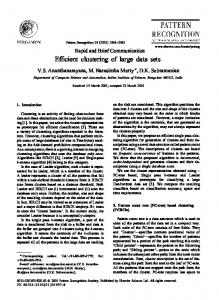
2. If Qmax = 2, sampling the posterior with Q = 2 will render the two clusters. 3. If Qmax > 2, sampling the posterior with Q = 2 will render two clusters that are nonintersecting combinations of the Qmax clusters. Both conjectures imply the hierarchical algorithm presented in Figure 1. The core of the hierarchical algorithm is the sampling algorithm described in Section 4.1. In the first iteration of the hierarchical algorithm it is used to split the whole sample of persons in two clusters. In all subsequent iterations, the sampling algorithm is i. used to split the largest cluster into two clusters, and ii. applied to all current clusters to allow between cluster transitions. If the expected number of persons in each resulting cluster is at least one, a new iteration (Q = Q ÷ 1 in Figure 1) is started. If at least one of the clusters is empty, the current iteration is repeated by splitting the next largest cluster (r = r + 1 in Figure 1). The hierarchical algorithm renders a sample from the global mode of the posterior distribution for Qmax clusters. Two issues deserve further attention: label switching (Stevens, 2000) and local modes (Richardson & Green, 1997). Both papers mainly consider mixtures of one variable. Although the theory in both papers can in principle be applied to model based clustering
d "l
Q=Q+I •
Q=O
r=0
sort the Q clusters from large to small and index them 1 ..... r ..... Q
r=r+l
randomly divide members cluster r over cluster r and Q+I and apply sampling algorithm
apply sampling algorithm to all Q+I clusters
yes
no
FIGURE 1. The hierarchical algorithm.
no
yes
488
PSYCHOMETRIKA
as discussed in this paper, the practical generalization to mixtures of 245 variables might not be easy. Local modes will be discussed in the next section. Interestingly enough, label switching is not a practical problem for mixtures of large numbers of variables. The probabilities computed in step 2 of the Gibss sampler are almost always close to zero or one, and hardly change from iteration to iteration. The implication is that there is only a small amount of between cluster migration across iterations of the Gibbs sampler, and that the majority of persons almost never leave the cluster they were allocated to in the initialization. As far as is known to the authors, the hierarchical algorithm is the first algorithm that is able to deal with outliers. If for response vector xi, P ( x i I ri = q) is small for all clusters, a cluster will be created containing only person i. As will be shown in the sequel, in the data at hand there were two outliers. 5. Determining the Number of Clusters
5.1. Global Modes and Local Modes Conjecture 1 presented in the previous section can be used to define the local modes of the posterior distribution of the cluster model: a local mode consists of Q < Qmax clusters, each corresponding to non-overlapping combinations of the Qmax clusters. Note that this definition implies that there are no local modes for Q = Qmax, and that empty clusters (see the first decision step in Figure 1) are excluded. Stated otherwise, for Q = Qmax a sample from the mode is sufficient for valid parameter estimation and goodness of fit evaluation. However, before analysis of the data the number of clusters in the population is unknown, which makes Q a (discrete) parameter instead of an ancillary statistic. In model based clustering and latent class analysis, it is common to estimate parameters and evaluate goodness of fit conditional upon the estimated value of Q. Although it is not unreasonable to report inferences for the best model, the uncertainty related to the estimation of Q is ignored. The latter is accounted for in the approach proposed by Richardson and Green (1997). In their reversible jump algorithm Q is a parameter that is sampled along with the class weights and class specific parameters. Richardson and Green (1997) illustrate their approach using mixtures of one variable. In their case the density of the variable implied by the mixture of mixtures with different Q can be used to summarize the sample of parameter vectors from the posterior distribution. However, with 245 variables (as is the case in our application) this is no longer possible. Using Conjecture 1, the number of mixtures (local and global maxima of the posterior distribution if Q is considered to be a parameter) can be computed. For Qmax = 4 this number is 14 (1 mixture of 4 clusters, 6 mixtures of 3 clusters in which two of the 4 clusters are combined, 6 mixtures of 2 clusters, and 1 mixture of 1 cluster). Presentation and interpretation of all these mixtures and their posterior weights will be impossible, especially if the number of clusters is large (in our application Qmax will turn out to be 19). This paper will adhere to the tradition in model based clustering and latent class analysis to describe and present the mode of the posterior distribution for an estimate of the number of clusters in the population, where the estimate is usually determined using goodness of fit tests and information criteria. The user's guide for Latent Gold (Vermunt & Magidson, 2000) contains examples of this approach on pages 88-90, 116, and 134-137. As will be elaborated below, in this paper the number of clusters is estimated using Qmax, a pseudo-likelihood ratio test and a Bayesian information criterion.
5.2. Qmax, Relative and Absolute Fit One of the challenges in model based cluster analysis is to determine the number of clusters. According to Conjecture 1 and Conjecture 2, the number of clusters in the data set at hand is equal
HERBERT
HOIJTINK
AND ANNELISE
NOTENBOOM
489
to Qmax. However, this is not necessarily the number of clusters in the population from which the data set is sampled. Determination of the number of clusters for large data sets containing many clusters is an under-explored area of statistics, and clear procedures and guidelines do not exist. For small data sets usually two approaches are combined to estimate the number of clusters in the population: information criteria (Lin & Dayton, 1997; Vermunt & Magidson, 2000, p. 61), and likelihood ratio tests (Everitt, 1988; Vermunt & Magidson, 2000, p. 61). In this paper the following criteria will be used to determine the number of clusters for the large data set at hand: 1. The number of clusters in the sample Qmax is used as the point of departure. 2. A Bayesian information criterion, (see Section 5.3) will be used to avoid over-fitting, that is, choosing a cluster model with too many clusters. If the Bayesian information criterion indicates that Qmax is too large, a smaller number of clusters will be chosen. 3. To avoid a cluster model that is not able to reconstruct the main features of the data set a pseudo-likelihood ratio test will be used (see Section 5.4). It will be computed for the number of clusters chosen using the Bayesian information criterion. Application of these criteria will render a reasonable estimate of the number clusters in the population. Whether or not these criteria can be improved upon is an area for further research. Before a description of the Bayesian information criterion and the pseudo-likelihood ratio test both will shortly be introduced using traditional information criteria and likelihood ratio test as the point of departure. Information criteria penalize the maximum of the likelihood for a specific number of clusters with the size of the cluster model. For AIC (Akaike, 1987) the penalty is a function of the number of parameters in the model, for CAIC (Bozdogan, 1987) and BIC (Congdon, 2001, pp. 472-474) the penalty is a function of the number of parameters and the sample size. Information criteria are relative fit measures. They can be used to determine which of a number of different models (here differing in the number of clusters) is the best. Likelihood ratio tests are absolute fit measures. The main components are the frequency with which each possible response vector x is observed and predicted (by the model at hand). Likelihood ratio tests are useless if the data set contains many items. Had the data been complete, for the data set at hand the number of possible response vectors would have been 2213s241°5537 (21 items had 2 response categories, etc.). It is clear that even with a sample size of N = 3614 this constitutes a very sparse contingency table. In this (complete data) situation the null-distribution of the likelihood ratio test is unclear (see, for example, Agresti, 1990, pp. 246-247). The situation is complicated further by the presence of data that are missing by design.
5.3. Relative Fit via the Marginal Likelihood The marginal likelihood (see Kass & Raftery, 1995, for a comprehensive overview) can be seen as a Bayesian information criterion. The interested reader is referred to Congdon (2001, pp. 4 7 2 4 7 4 ) who derives the BIC from the marginal likelihood assuming a multivariate normal likelihood function and a prior that is worth one observation. The marginal likelihood functions as a fully automatic Occam's razor (Smith & Spiegelhalter, 1980). Stated otherwise, although not directly visible from the formulation of the marginal likelihood (5), it does account for model complexity. For a general discussion, illustration and further references the interested reader is referred to Hoijtink (2001), Berger and Pericchi (2001), and Jefferys and Berger (1992). In the sequel, minus twice the logarithm of the marginal likelihood will be used. This brings it on the same scale as the traditional information criteria ~ 2 ~0 g
f P ( X ] Q, z, M) = - 2 l o g [ g(X ] 0 Q, z,M)h(oQ), J
oQ
(5)
490
PSYCHOMETRIKA
where 0 Q denotes the parameters of a cluster model with Q clusters. Note that the computation of (5) is not hindered by the presence of missing data. However, due to the integral computation is not easy. According to Hoijtink (2001) stable estimates of (5) are obtained using an idea that can be found in Newton and Raftery (1994) and Kass and Raftery (1995). They propose to sample 1 - c~% parameter vectors from the posterior distribution of a cluster model with Q clusters, and to sample c~% from an imaginary distribution where each parameter vector has a density equal to the marginal likelihood. Subsequently, solution of the implicit equation [
_ :
r~,r
g(X I 0 Q, z, M)
'~
renders an estimate - 2 l o g / ; of (5). The interested reader is referred to Hoijtink (2001) for a solution algorithm that converges quickly. The smaller minus twice the logarithm of the marginal likelihood, the better the corresponding number of clusters. The interested reader is referred to Kass and Raftery (1995) who give guidelines for the interpretation of differences in the size of (5) for different models. 5.4. Absolute Fit via the Pseudo-Likelihood Ratio Test 5.4.1. Dealing with Large Data Sets The pseudo-likelihood ratio test (7) is a discrepancy measure (Meng, 1994), that is, a test statistic that is a function of both the data and the unknown model parameters.
kj jC=j: v = l
(e(xj =
-2 [ o,))
w=l
(7) where
E(xj =v,x/=w l Tr,oJ)=~-]zwvjlqzwwjlq( ~
Pq]i).
(8)
'lmij=l,mij/=l Note that N(.) and E(.) denote the observed and expected number of persons responding according to the argument, and that ~ilmij=l,mij/= 1 Pqli denotes the expected number of persons in cluster q responding to both items j and j:. Where the likelihood ratio test evaluates whether the observed frequency of each possible response vector x can be predicted by a model with Q clusters, the pseudo-likelihood ratio test focuses on two-dimensional summaries of expected and observed frequencies of the J-dimensional contingency table. The implication is that it ignores three-way and higher-order interactions among the J items, and that it only evaluates whether main effects and two-way interactions are adequately predicted. It is safe to state that a good cluster model should be able to predict main and two-way interaction effects. Whether this is enough is to a large extent an open question. Simulations by Hoijtink (1998, 2001) indicate for sparse contingency tables that the pseudo-likelihood ratio test has a better performance than the likelihood ratio test.
HERBERT HOIJTINK AND ANNELISE NOTENBOOM
491
5.4.2. Dealing with Missing Data Using Expunction Formal hypothesis testing in the presence of missing data is usually based on multiple imputation (Rubin, 1987; Schafer, 1997; Schafer & Graham, 2002). However, multiple imputation cannot be used to evaluate most goodness of fit tests, that is, tests that address "fixed" properties of a model like normality, linearity and homoscedasticity. The consequence for model based cluster analysis is that multiple imputation cannot straightforwardly be used to deal with questions like "how good is the fit of a model with (2 clusters," and, "how good is the fit of a model assuming conditional independence of the item responses within each cluster." As will be elaborated below, data expunction is a novel idea that can be used to evaluate the pseudo-likelihood ratio goodness of fit test introduced in the previous subsection. However, this can only be done if researchers are willing to develop special purpose software (as was done for this paper) in order to be able to execute the required analyses. Data expunction does not impute the missing values, which makes it suited for goodness-of-fit evaluation. However, further research is needed to determine its usefulness for the evaluation of hypotheses with respect to model parameters. Data expunction evaluates model-fit using only the observed data. The main difference with multiple imputation is the "expunction" of data from matrices X rep replicated from the null population, instead of imputation of missing data in the observed data matrix X. Both for data expunction and multiple imputation it holds that the resulting inferences are only valid if the missing data mechanism is known. In our application the data are missing by design based on the grade of a pupil (see Table 1). This implies that the missing data mechanism is exactly known. The pseudo-likelihood ratio discrepancy measure (7) can be evaluated using posterior predictive p-values (Gelman, Carlin, Stern & Rubin, 2000, pp. 167-173; Meng, 1994) if the missing data mechanism is explicitly accounted for: P ( D ( X rep, z, M, ~, ~o) > D(X, z, M, ~, ~o) I X, z, M),
(9)
where M is an N × J design matrix in which a 0 indicates that an item response is missing by design, and a 1 that an item response is observed. As can be seen, only the observed data (and their replicated counterparts) are used in (9). It is evaluated with respect to the distribution of the three random variables X rep, "tr and ~o: g( xrep, ~, ~ I X, z, M) = g ( X rep I ~, ~ , z, M ) Post(Tr, ~o I X, z, M).
(10)
As can be seen (10) decomposes into two parts that each account for the missing data mechanism represented by M. The density of X rep is defined for the values that are observed as indicated by M. The posterior distribution of 7r and ~o also accounts for M. This posterior is a valid basis for inference, since conditional on grade the data are missing completely at random. A four-step simulation is used to actually compute (9): 1. For t = 1 . . . . . T sample 0t from (4). 2. For t = 1 . . . . . T sample X~ep from (1). This can be done in two sub-steps: (i) sample the complete X~ep, and (ii) use M to delete the entries that are missing by design. 3. For t = 1 . . . . . T compute D(X~ ep, z, M, Ot) and D(X, z, M, Or). 4. Compute the proportion D(X~ ep, z, M, Ot) > D(X, z, M, Or). 6. The Number of Clusters and Developmental Stages The hierarchical algorithm presented in Section 4.2 rendered 19 clusters. Stated otherwise, it was not possible to create 20 clusters such that the expected number of persons in each cluster
492
PSYCHOMETRIKA TABLE 2. Determining the number of clusters
Number of clusters
p-value Pseudo likelihood
- 2 log Marginal likelihood
12 13 14 15 16 17 18 19
.00 .01 .02 .04 .11 .11 .16 .16
539551 538990 538887 538187 537789 537108 535622 535000
was larger than one. A c c o r d i n g to the criteria presented in Section 5.2, the marginal likelihood will be used to avoid over-fitting resulting from the use of (2max = 19 clusters. As can be seen in Table 2, the marginal likelihood is at its m i n i m u m for 19 clusters and thus there is no indication of over-fitting. The p s e u d o - l i k e l i h o o d ratio test is used to ensure that 19 clusters is enough to reconstruct the main features of the data. As can be seen in Table 2, the p - v a l u e of .16 indicates that 19 clusters are sufficient to m o d e l the data. The n u m b e r of pupils per cluster is given in Table 3. For i = 1, . . . , N each pupil was assigned to the cluster for which Pqli was the highest. In order to be able to evaluate the stage m o d e l and the m o d e l of overlapping waves, the clusters h a v e to be ordered along a d e v e l o p m e n t a l d i m e n s i o n representing spelling skills. As can be seen in c o l u m n 2 of Table 3, the average grade
TABLE 3.
For each duster proportion of pupils per grade and total number of pupils Cluster number
Average grade
1
1
1
1.00
2 3 4 5 6 8 7 9 10 11 12 13 14 15 16 17 Outlier 1 Outlier 2
1 1 1 1 1 1.5 1.8 2.1 2.4 3.2 3.5 3.6 4.8 5.3 5.7 5.7 1 6
.99 1.00 1.00 1.00 1.00 .45 .25 .03 .02
Total
Grade 2
3
4
5
6
.01
.55 .70 .88 .61
.05 .09 .34 .82 .47 .53
.03 .18 .52 .37 .39
.01 .08 .43 .73 .34 .29
.02 .18 .27 .66 .71
1.00 1.00 577
657
603
557
615
605
Total 66 91 24 90 82 109 164 96 296 391 51 392 403 477 230 326 324 1 1 3614
HERBERT
HOIJTINK
AND ANNELISE
NOTENBOOM
493
of the cluster members is used to order the clusters. To order clusters 1-6 which all have the same average grade (ignoring 1 pupil in cluster 1 that is a second grader), the proportion of correct responses to items 1-84 is used. As can be seen in Table 3 the order obtained is validated because the distribution of cluster members over the grades shows a nice parallelogram structure with one top per cluster. This structure should appear if the ordering of the clusters represents an ordering with respect to a developmental dimension (spelling skills). The lower cluster numbers contain without exception pupils with a low grade (spelling ability). The higher cluster numbers contain without exception pupils with a high grade (spelling ability). Also clusters 10-13 contain mainly pupils with an average grade. Stated otherwise, each cluster is associated with a homogeneous range of grades. Two of the 19 clusters had only one member. They were outliers, and their response patterns were very different from the rest of the data. For most children, learning irregular sound-letter mappings did not affect their spelling of regular words. This was not true, however, for outlier 1, who spelled regular words in an erratic way. Outlier 2 was a sixth grader with rather low spelling skills. Since there is no overlap in the items given to the first and sixth graders, this child became a cluster by itself: there are no other children responding to about the same subset of items that have about equal spelling skills. 7. Evaluation of Clusters Excluding the outliers, an interpretation of the 17 remaining clusters involves an evaluation of roughly 5 x 17 x 245 ~ 20,000 cluster specific probabilities. To be able to do this the clusters have been ordered using the average grade of the pupils in each cluster, figures will be given for clusters 1-10, and clusters 10-17. The reason for the split is that the overlap of items is too small for a comparison of clusters 1 through 17. Figures 2 and 3, which will be discussed in the next section, will be used to discuss the results for clusters 1-10. Figures 4 and 5 will be used to discuss the results for clusters 10-17. The figures give only a part of the results obtained in this study. In each figure, for each cluster the probability of (some of) the five possible responses to subsets of the items will be given. To give an example, in Figure 2 it can be seen that the proportion of semiphonetic responses to items 1-84 was about .40 in cluster 3. Figures 2 and 4 are used to evaluate the stage model and the model of overlapping waves, and Figures 3 and 5 are added to further illustrate the results. For a complete overview of these (nonstatistical) results and conclusions, the interested reader is referred to Notenboom, Hoijtink, and Reitsma, 2004. Z1. Clusters 1-10
In Figure 2 for items 1-84 the proportion responses given to each of four possible response categories are presented for clusters 1-10. Transitional responses are not possible for these items and are thus not included in Figure 2. The first cluster depicted in Figure 2 has a high proportion of responses indicative of the semiphonetic stage. This proportion decreases rapidly over subsequent clusters, whereas the proportion correct increases concurrently. Responses indicative of the phonetic stage show a typical non-linear pattern. At the beginning of development, children do not know how sounds can be represented by letters; then they master this principle, and subsequently, they learn the irregular forms as well. If the criteria from Section 2 are applied, Figure 2 is more supportive of the model of overlapping waves than for the stage model. Although it is clear that the first two clusters can be characterized by semiphonetic responses and the last two clusters by correct responses, none of the other clusters can be characterized by the use of only one response category. Furthermore, changes among clusters occur gradually, not instantly. Finally, although in the beginning of development semiphonetic responses are dominant, this is later not followed by a dominance of
PSYCHOMETRIKA
494 1.0
Correct
0.8 e.,
©
e., ©
g,
0.6
Semiphonetic
at
0.4
Phonetic
0.2 Other error 0.0
i
i
1
2
i
3
i
i
4
i
5
6
i
i
7
8
i
9
10
Cluster FIGURE 2. Summary of the results for clusters 1-10, for items 1-84.
phonetic responses. A t higher levels of d e v e l o p m e n t there is no p r e f e r e n c e for semiphonetic or phonetic responses. To elaborate and further illustrate these results, in F i g u r e 3 the response curves for the w o r d beste are displayed; the second e of this w o r d is silent. A t the onset of development, children are not able to represent all sounds of the w o r d adequately, resulting in a high proportion of semiphonetic responses. Subsequently, children spell the w o r d either phonetically (e.g., bestu) or semiphonetically, and finally m a i n l y correct responses are given. T h e s e results are along the s a m e lines as the results obtained for all 84 items displayed in F i g u r e 2.
0.8 ©
ca
--
0.6 ." o ° ° , •,
~D ©
Correct •
Semiphonetic
....
Phonetic
0.4
g, 0.2
i
1
i
2
i
3
i
4
i
5
i
" ' ~ ' ' ' ~ ' ' q P "
6
7
8
i
9
10
Cluster FIGURE
3.
Zooming in on the results for clusters 1-10, the spelling of the word beste.
495
HERBERT HOIJTINK AND ANNELISE NOTENBOOM
7.2. Clusters 10-17
Responses indicative of the transitional stage were present for two types of items, administered to the second and higher grades. One type of items involved the application of spelling rules; the other type of items contained irregular letter-combinations. Presented in Figure 4 are response proportions for the response categories of the latter type of items (a total of 46) only. If the criteria from Section 2 are applied, Figure 4 is more supportive of the model of overlapping waves than for the stage model. None of the clusters can be characterized by the consistent occurrence of just one response category. Both the phonetic and transitional response categories are used fairly often, although at higher levels of development mainly correct responses are given. Stated otherwise, there are no clusters that consistently prefer one of the response categories. Furthermore, there is no clear developmental sequence in prevalence of error-types along the continuum. Changes occur gradually, but not smoothly. This is probably a result of the use of grade to order the clusters along a developmental continuum. An ordering based on the proportion of correct responses within each cluster would have rendered smooth curves. However, the parallelogram structure presented in Table 3 would then have been lost. A potential solution for this problem is to restrict the cluster model used to render a one-dimensional ordering of clusters. However, this an area for future research. To elaborate and further illustrate these results, the response curves for a subset of three items including the letter combination eau, administered at the fourth and higher grades, are presented in Figure 5. As can be seen, semiphonetic responses are dominant for cluster 11, whereas phonetic responses, like nivoo for niveau (level), are characteristic for the clusters 10, 12, 13 and 15. For clusters 14 and 16 the proportion of phonetic and transitional responses (like nivau or nivea) are rather similar, and in clusters 11 and 15 phonetic spelling is dominant although transitional spelling is also used. Again, most clusters do not consistently use one response strategy, changes occur gradually, and there is no clear developmental sequence in prevalence of errortypes along the continuum. The results in Figure 4 and 5 provide more support for the model of overlapping waves than for the stage model.
0.8
Correct
©
Semiphonetic
0.6
©
A
Phonetic
....
Transitional
0.4 Other error
0.2
i
10
i
11
i
12
i
13
i
14
i
15
i
16
i
17
Cluster FIGURE 4. Summary of the results for clusters 10-17, for 46 items containing irregular letter combinations.
496
PSYCHOMETRIKA
0.9
Semiphonetic spelling of words with e a u
......
0.8 0.7 ©
Phonetic spelling of words with e a u
0.6 0.5
Transitional spelling of words with e a u
A
0.4 ©
0.3 0.2 0.1 0
i
10
i
11
i
12
i
13
i
14
i
15
i
16
i
17
Cluster FIGURE 5. Zooming in on the results for clusters 10-17, three items containing the letter combination
eau.
8. Research Questions and Answers Stage theory predicted clusters corresponding to the semiphonetic, phonetic, transitional and correct stages specified before. Model based clustering rendered 17 clusters (excluding the two outliers). Most of these clusters could not be characterized by the consistent occurrence of one response category. It could be seen that the dominance of the response categories changed gradually along the developmental spectrum, although the sequence predicted by stage theory was not always clearly visible. In clusters 1-3, responses are mainly inadequate approximations of the sound structure, indicative of the semiphonetic stage. Children in clusters 4-8 produced mainly an adequate (although in the case of irregular words incorrect) rendering of the sound structure of words, characteristic for the phonetic stage. Nevertheless, semiphonetic spellings are still current at a moderate level. Children in clusters 9 and 10 mainly responded correctly to the 84 easiest items of the spelling test. At clusters 10-15 both phonetic and transitional responses are given. In clusters 16 and 17 mainly correct responses are given. Although stage theory provides a rough description of the developmental trajectory presented in Figures 2 to 5, the basic assumptions are untenable. There was no clear succession in error-types found along the developmental continuum. Furthermore, the variety of response strategies found for the clusters, and the gradual changes between the clusters, fit better in the developmental paradigm of overlapping waves. The interested reader is referred to Notenboom, Hoijtink, and Reitsma (2004) for a nonstatistical elaboration of the main results presented here. 9. Discussion This paper presented a model based clustering or latent class approach for the analysis of a large data set of which part was missing by design. A number of problems had to be solved in order to be able to analyze this data set. First of all, an algorithm that is able to handle large data sets and renders only non-degenerate clusters was proposed. Secondly, a pseudo-likelihood ratio test that is not affected by the fact that the number of possible response vectors is by far out-
HERBERT HOIJTINK AND ANNELISE NOTENBOOM
497
weighted by me number of observed response vectors was proposed. Thirdly, a novel approach, "data expunction," that enables the computation of a p-value if the missing data mechanism is known was proposed. The resulting model based clustering approach was applied to data with respect to the development of spelling skills. The conclusion was that the results are more in accordance with the paradigm of overlapping waves than with the stage model. Although this paper shows that the approach proposed is viable, research with respect to the clustering of large data sets is not finished. Possible avenues of further research are: providing a proof for Conjectures 1 and 2; studying the frequency properties of the posterior predictive p-value computed for the pseudo-likelihood ratio test; a further study of the marginal likelihood and its role in determining the number of clusters; extension of the cluster model such that it renders clusters that are located in a low dimensional space; and, a study of simple summaries of the huge amount of information that results from the model based clustering of large data sets. However, each of these will be the topic of separate and future papers. References Agresti, A. (1990). Categorical data analysis. New York: John Wiley. AkaJke, H. (1987). Factor analysis and AIC. Psychometrika, 52, 317-332. Berger, J., & Pericchi, L. (2001). Objective Bayesian methods for model selection: Introduction and comparison [with discussion]. In: P. Lahiri (Ed.), Model selection, Lecture Notes Monograph Series Volume 38 (pp. 135-207). Beachwood, OH: Institute of Mathematical Statistics. Bear, D.R. & Templeton, S. (1998). Explorations in developmental spelling: Foundations for learning and teaching phonics, spelling and vocabulary. The Reading Teacher, 52, 222-242. Bowman, M., & Treiman, R. (2002). Relating print and speech: The effects of letter names and word position on reading and spelling performance. Journal of Experimental Child Psychology, 82, 305-340. Bozdogan, H. (1987). Model selection and AkaJke's information criterion (AIC): The general theory and its analytical extensions. Psychometrika, 52, 345-370. Congdon, R (2001). Bayesian statistical modelling. New York: John Wiley. Ehri, L. (1986). Sources of difficulty in learning to spell and read. In: M.L. Wolraich and D. Routh (Eds.), Advances in developmental and behavioralpediatrics, Vol. 7 (pp. 121-195). Greenwich, CT: JAI Press. Everitt, B.S. (1988). A Monte Carlo investigation of the likelihood ratio test for number of classes in latent class analysis. Multivariate Behavioral Research, 23, 531-538. Frith, U. (1980). Unexpected spelling problems. In: U. Frith (Ed.), Cognitive processes in spelling (pp. 495-515). London: Academic Press. Frith, U. (1985). Beneath the surface of developmental dyslexia. In: K.E. Patterson, J.C. Marshall, and M. Coltheart (Eds.), Surface dyslexia (pp. 301-326). London: Routledge and Kegan-Paul. Geelhoed, J., & Reitsma, R (1999). PI-dictee. Lisse: Swets and Zeitlinger. Gelman, A., Carlin, J.B., Stern, H.S., & Rubin, D.B. (2000). Bayesian data analysis. London: Chapman and Hall. Gentry, J.R. (1982). An analysis of developmental spelling in GNYS AT WRK. The Reading Teacher, 36, 192-200. Henderson, E.H., & Templeton, S. (1986). A developmental perspective of formal spelling instruction through alphabet, pattern and meaning. The Elementary School Journal, 86, 305-316. Hoijtink, H. (1998). Constrained latent class analysis using the Gibbs sampler and posterior predictive p-values: Applications to educational testing. Statistica Sinica, 8, 691-711. Hoijtink, H. (2001). Confirmatory latent class analysis: Model selection using Bayes factors and (Pseudo) likelihood ratio statistics. Multivariate Behavioral Research, 36, 563-588. Hoskens, M., & de Boeck, E (1995). Componential IRT models for polytomous items. Journal of Educational Measurement, 32,364-384. Hoskens, M., & de Boeck, E (1997). A parametric model for local dependence among test items. Psychological Methods, 2, 261-277. Jefferys, W., & Berger, J. (1992). Ockham's razor and Bayesian analysis. American Scientist, 80, 64-72. Kass, R.E., & Raftery, A.E. (1995). Bayes factors. Journal of the American Statistical Association, 90, 773-795. Lin, T.H., & Dayton, C.M. (1997). Model selection information criteria for non-nested latent class models. Journal of Educational and Behavioral Statistics, 22, 249-264. Meng, X.L. (1994). Posterior predictive p-values. The Annals of Statistics, 22, 1142-1160. Morris, D., Nelson, L., & Perney, J. (1986). Exploring the concept of "spelling instructional level" through the analysis of error-types. The Elementary School Journal, 87, 181-200. Newton, M.A., & Raftery, A.E. (1994). Approximate Bayesian inference with the weighted likelihood bootstrap. Journal of the Royal Statistical Society, B, 56, 3-48. Notenboom, A., Hoijtink, H., & Reitsma, E (2004). Modeling the development of Dutch spelling ability by Latent Class Analysis. Manuscript submitted for publication.
498
PSYCHOMETRIKA
Richardson, S., & Green, EJ. (1997). On Bayesian analysis of mixtures with an unknown number of components. Journal of the Royal Statistical Society, B, 59, 731-792. Rittle-Johnson, B., & Siegler, R.S. (1999). Learning to spell: Variability, choice and change in children's strategy use. Child Development, 70, 332-348. Rubin, D.B. (1987). Multiple imputation for nonresponse in surveys. New York: John Wiley. Scha£er, J.L. (1997). Analysis of incomplete multivariate data. London: Chapman and Hall. Scha£er, J.L., & Graham, J.W. (2002). Missing data: Our view of the state of the art. Psychological Methods, 7, 147-177. Siegler, R.S. (1995). How change does occur: A microgenetic study of number conservation. Cognitive Psychology, 28, 225-273. Siegler, R.S. (1996). Emerging minds: The process of change in children's thinking. New York: Oxford University Press. Siegler, R.S. (2000). The rebirth of children's learning. Child Development, 71, 26-35. Siegler, R.S., &Chen, Z. (1998). Developmental differences in rule learning: A microgenetic analysis. Cognitive Psychology, 36, 273-310. Siegler, R.S., & Stern, E. (1998). Conscious and unconscious strategy discoveries: a microgenetic analysis. Journal of Experimental Psychology: General, 127, 377-397. Smith, A.F.M., & Spiegelhalter, D.J. (1980). Bayes factors and choice criteria for linear models. Journal of the Royal Statistical Society, Series B, 42, 213-220. Steffler, D.J., Varnhagen, C.K., Treiman, R., & Friesen, C.K. (1998). There's more to children's spelling than the errors they make: Strategic and automatic processes for one-syllable words. Journal of Educational Psychology, 90, 492505. Stevens, M. (2000). Dealing with label switching in mixture models. Journal of the Royal Statistical Society, Series B, 62,795-810. Treiman, R., & Bourassa, D.C. (2000). The development of spelling skill. Topics in Language Disorders, 20, 1-18. Varnhagen, C.K., McCallum, M., & Burstow, M. (1997). Is children's spelling naturally stage-like? Reading and Writing: An Interdisciplinary Journal, 9, 451-481. Vermunt, J.K., & Magidson J. (2000). Latent Gold. Belmont: Statistical Innovations Inc. Zeger, S.L., & Karim, M.R. (1991). Generalized linear models with random effects: A Gibbs sampling approach. Journal of the American Statistical Association, 86, 79-86.
Manuscript received 11 APR 2004 Final version received 14 SEP 2004