Thus the gain term doesn't contain the Laplace variable s. ... the last 1-junction for rope dynamics (connected to bonds 9,10 and 11) is modeled .... Let us define only one observed output as the velocity of the hung-mass, or the variable f8. ... rolling (without slip) and further neglect the rolling friction with the ground. The.
Chapter 3
Model-based Control
3.1 Introduction A control system refers to a set of devices used to manipulate the output of a system by altering its inputs, called commands. There are two types of control systems: manual and automatic. We will devote our discussion to the latter in this chapter. The desired or prescribed system output is called the reference. A controller manipulates the inputs to a system to obtain the desired effect on one or more outputs of the system, which are speci ed as different references. As an example, consider the speed control of an electric automobile in cruise mode. In this case, the reference behavior is speci ed as a constant vehicle speed. The input variable is the armature current of the drive motor, which regulates the driving torque. As we have discussed before, the electric current and mechanical torque are represented by a GY element in bond graphs, which also relates the motor speed to the back emf. The motor speed changes depending on the roughness and elevation (upward or downward slope) of the road as well as other external factors such as tail wind, tyre pressure, ambient temperature, etc. This means that during motion the vehicle will not be able to move at constant speed without changing its torque output, which consequently means without altering armature current of the motor. For this purpose, one needs to take note of the vehicle's velocity and modify the armature current accordingly. Such a system requires simultaneous use of sensors, controllers and actuators, and is called a closed-loop feedback control system. The controller monitors the vehicle's speed and appropriately adjusts the armature current to maintain the desired speed. The feedback compensates for disturbances to the system, such as changes in slope of the ground, road roughness, wind speed, etc. A control system needs to be robust, i.e. it should be responsive to commands whereas it should not be affected by minor changes in system parameters and external disturbances. A robust controller should achieve its objective (reference tracking) even if the mathematical model used to design it is little imperfect. This is because no real physical system would truly behave according to its behavioral model (the set of differential equations). Moreover, controller design is usually based on re-
81
82
3 Model-based Control
duced order system models; the simpli cation of mathematical models is necessary for arriving at simpler and implementable control laws as well as for fast computation (in computer or microprocessor based digital control). Furthermore, even when a perfect mathematical model of a system is used to design its controller, the numerical parameter values cannot be determined with absolute precision, i.e. there will always be some measurement or estimation error. Therefore, a robust controller will have to behave correctly even when the connected physical system's parameter values are marginally different from their corresponding nominal parameter values used in the controller synthesis. An adaptive control strategy uses on-line system identi cation and estimation of the process parameters, or modi cation of controller gains, so that strong robustness properties are obtained. The advantages of closed-loop controllers over manual and open-loop controllers may be summarized as follows: 1. Disturbance rejection 2. Robustness with respect to process and measurement uncertainties, low sensitivity to process parameter changes 3. Stability of the processes 4. Better trajectory or reference behavior tracking Some control systems implement simultaneous closed-loop and open-loop (feedforward) control, where the open-loop control helps improve the reference tracking performance. One commonly used closed-loop controller is the PID (proportional-integral and derivative) controller. If the PID controller parameters, i.e. the proportional, integral and derivative gains, are improperly chosen, then the controlled process may become unstable or show steady/unsteady utter behavior. Therefore, one needs to adjust optimally the controller gains, either statically or dynamically, to obtain the desired system response. Such adjustments are called tuning of the control loop. Improperly tuned controllers are inef cient, inaccurate, and often dangerous. Some controllers implement automatic tuning, e.g. a self-tuning PID controller. The tuning speci cations may change from system to system depending upon its response time; while guarantying stability of the system without oscillations. Some process may require that there will be no overshoot above the setpoint while some other process may require minimizing the time or energy spent in reaching the setpoint. In process engineering systems, which are generally non-linear, PID controller gains need to be adjusted all along the start up and shut down process as well as when the setpoint changes. One of the of ine tuning method of a PID control loop involves experimentally cataloguing step response of the system at different operating conditions with different gain combinations and using a database to store this information, which would be later used during online process operation. Two of the well known online methods are Ziegler-Nichols method and Cohen-Coon method. Sometimes feedback systems are constructed as subsystems and then they can be combined in many ways. This way of design offers exibility of choice as well as the exibility of switching between controllers. One example is the series connection
3.1 Introduction
83
of two controllers, referred to as cascaded control, where one control loop tries to maintain a setpoint, but then its output becomes a setpoint to another controller instead of becoming an actuating signal to an actuator. The second controller may have another setpoint and then it may act on the actuator. This way, usually two or more dynamically related process variables (e.g. temperature and pressure) are simultaneously controlled. In process engineering, one has to control many process outputs and most often some of them are strongly coupled. The class of control strategies followed in this case is called a multivariable control. Model predictive control, or MPC, is one of the multivariable control methods. Many chemical process plants, power plants and oil re neries use MPC. One of the requirements of designing an MPC system is the availability of a well developed process model, which may be either analytical or empirical (e.g. by system identi cation, statistical analysis or training of a neural network model). These models are used to predict the process behavior and output with respect to the changes in the input process parameters. As an example, the weld bead geometry and strength of the welded joint may be the output parameters while pulse frequency, pulse voltage, background voltage, wire feed rate, table feed rate, and inert gas pressure, etc. may be the input parameters in an automated pulsed metal inert gas (PMIG) welding system. In chemical batch production processes, input parameters are generally setpoints of controllers actuating various valves (valve positioners) and heating and stirring elements, while the output variables are generally the process constraints, maximum productivity, product quality, safe operation limits.. Obviously, MPC has to be developed from optimality principles. An MPC system uses the process model and measurements from different sensors to precalculate the required changes in the setpoints such that operational constraints are satis ed. To summarize, an MPC algorithm is an iterative nite horizon optimization of a plant model. At every sampling time, a numerical optimization algorithm computes the commands for a very short time span. The rst step of this calculated command is then implemented and the output is sampled to be used again in the optimization algorithm. This way, the prediction horizon keeps on shifting forward. Therefore, MPC is also called receding horizon control. Because of the fact that MPC algorithms are executed at every sampling step, they must be very fast; i.e. they should be able to converge before the next sampling step. Creating such software for real time implementation is a specialized task. Honeywell, AspenTech, and Emerson are some of the well-known MPC software vendors; they also customize their software for the speci c process. One of the basic objectives of a control system is to ensure stability of the closedloop behavior at all times. In linear systems, this may be achieved through direct feedback control or pole placement. However, non-linear systems pose great degree of dif culty in controller design because they may have multiple equilibriums (stable/unstable nodes, foci and saddle points), they may exhibit limit cycle, bifurcation and chaos behavior, their response may contain several sub and super harmonics of the input frequency and nally, they do not respect the principle of superposition. Stability of non-linear systems is often de ned by Lyapunov's stability criterion,
84
3 Model-based Control
which tests the asymptotic stability of the output while disregarding the internal system dynamics. However, every process has some constraints on its internal variables. It is sometimes possible to linearize piece-wise a non-linear system's model and then apply linear control techniques, such as gain scheduling control and adaptive control. Some control systems introduce auxiliary non-linear feedback in such a way that the system can be treated as linear for purposes of controller design, e.g. feedback linearization control. However, in many cases, speci c control strategies are developed for speci c non-linear systems. Such control strategies usually try to achieve stability in the Lyapunov sense, e.g. back-stepping control and sliding mode control. From the preceding discussions, we understand that a well-developed model is a prerequisite for development of its control system. In this chapter, we will illustrate some of the physical model based control strategies. Moreover, we will emphasize the structural properties of systems which can aid in the preliminary design of control strategies and to foresee some of the problems in implementing the control algorithm. These theories establish certain thumb-rules to design quickly the required instrumentation architecture for speci c control systems.
3.2 Classical Model-based Control 3.2.1 Conversion of Bond Graph Models to Signal Flow Graph Models Bond graphs for linear systems can be easily converted to signal ow graphs (SFG) and transfer functions between inputs and outputs can be obtained for further analysis with linear control theory. The procedure for such conversion is laid out here. 3.2.1.1 Nodes of SFG (Junction Laws) A signal ow graph is constituted of nodes connected by a set of directed lines called branches or edges. Each branch has an associated gain and each node signi es an algebraic sum. Unlike bond graphs, SFGs do not have any power direction (the coordinate system is represented by gains +1 and 1), but causality is portrayed by the direction of the edges. Therefore, an SFG is a linear causal graph. The branches in an SFG simply specify traversal path and are associated with only one signal. Each bond in a bond graph is thus represented by two nodes in an SFG (effort and ow node). Activated or signal bonds are represented by only one node.
3.2 Classical Model-based Control
85
All bonds connected to a 1-junction have the same ow and are thus represented by a single ow node. Similarly, all bonds connected to a 0-junction are represented by a single effort node. The nomenclature for a ow node representing ows in bonds of a 1-junction is fi; j;k , where i; j; k,... are the bond numbers of bonds connected to that junction. A common effort node for bonds at a 0-junction is similarly represented by ei; j;k;::: . All bonds connected to a 1-junction contribute separate effort nodes (viz, ei , e j ,... where i; j;.. are bond numbers) leaving apart those which have been already represented in SFG. Similarly, All bonds connected to a 0-junction contribute separate ow nodes (viz, fi ; f j ... where i; j; ::: are bond numbers) except those which have been already represented in SFG. 3.2.1.2 Branches and Gains (Constitutive Relations) R
For an I-element in integral causality, the equation is f = m 1 edt + f0 : Because of the fact that initial conditions cannot be considered in the frequency domain, the term f0 is neglected. Taking the Laplace transform, f (s) = e(s)=(ms) or f (s)=e(s) = 1=(ms). Thus the gain associated with an integrally causalled I1 element is ms while the branch is directed from the effort to the ow node (cause to effect). Similarly, for a differentially causalled I-element, the gain is ms and the branch is directed from the ow to the effort node. Cause Rand effect relation for an integrally causalled C-element is given by e = K f dt + e0 . Taking the Laplace transform of both sides, e(s) = Ke(s)=s or e(s)= f (s) = K=s. Thus the gain associated with an integrally causalled C1 element is K=s (or Cs ) while the branch is directed from the ow to the effort node (cause to effect). For a differentially causalled C-element, the gain is s=K and the branch is directed from the effort to the ow node. The relationship between the cause and the effect for R-elements is not described by differentiation or integration. Thus the gain term doesn't contain the Laplace variable s. The gain for the R-element in resistive causality is e(s)= f (s) = R whereas, for conductive causality, it is f (s)=e(s) = 1=R. Similar relationships can be established for two-ports TF and GY. The bond graph elements in different causalities and their corresponding signal ow graph representations are shown in Table 3.1.
3.2.1.3 Receptors (Junction Algebra) The 1-junction is a ow equalizing and effort sum junction. The strong bond for the 1-junction is the bond that has causality away from the junction. This strong bond thus provides information of ow to the junction. The weak variables of the 1-junction are efforts. The effort equation for the 1-junction is written for the weak variables (efforts), where the effort in the strong bond is expressed as
86
3 Model-based Control
Table 3.1 Signal ow graph of bond graph elements Bond graph
Signal ow graph
signed sum of efforts in other bonds. This weak effort variable of the strong bond is called the receptor of the junction. For the 1-junction shown in Figure 3.1 the junction algebra equation is e2 = e1 e3 . The signal ow graph representation is shown to the right of Figure 3.1.
Fig. 3.1 SFG representation of 1-junction
3.2 Classical Model-based Control
87
Bond number 2 is the strong bond and the weak variable e2 is the receptor node. Signals from other nodes for weak variables are added to this node. The gain for all branches in SFG corresponding to bonds that are power directed in opposite direction as compared to the strong bond (i.e. counter-oriented) is 1. Otherwise, i.e. for all co-oriented bonds (bonds having same power orientation as the strong bond as seen from the junction), the gain is 1. The receptor for a 0-junction is the weak ow variable of the strong bond (the bond that decides effort of the 0-junction, i.e. causalled near the junction). For the 0-junction shown in Figure 3.2, the junction algebra can be represented at the receptor node f2 as shown to the right of Figure 3.2.
Fig. 3.2 SFG representation of 0-junction
3.2.1.4 Example Let us consider an electromechanical system whose schematic diagram and bond graph model are shown in Figure 3.3. In the rst step, the left-most 1-junction and elements connected to it in the bond graph model are considered. Node e1 represents the input source. The part SFG is shown in Figure 3.4.
(a) Fig. 3.3 A DC motor driven rotor
(b)
88
3 Model-based Control
Fig. 3.4 First step in SFG construction
The next junction considered is the 1-junction for disk's angular velocity connected to bonds 4, 5 and 6. The resulting part SFG is shown in Figure 3.5.
Fig. 3.5 Second step in SFG construction
The gyrator between the two 1-junctions is then represented in SFG (Figure 3.6).
Fig. 3.6 Third step in SFG construction
In Figure 3.7, the next junction in the bond graph model (0-junction connected to bonds 7, 8 and 9) is represented in the SFG. The transformer representing rotational to linear velocity transform is then represented in the SFG in Figure 3.8. Thereafter, the last 1-junction for rope dynamics (connected to bonds 9,10 and 11) is modeled in SFG as shown in Figure 3.9. Now the system has been completely represented as a signal ow graph. All available effort and ow nodes have been added. Signal from any ow node can be
Fig. 3.7 Fourth step in SFG construction
3.2 Classical Model-based Control
89
Fig. 3.8 Fifth step in SFG construction
Fig. 3.9 Signal ow graph model of the example system
integrated (gain = 1=s) to represent a displacement node as shown in Figure 3.10. Similarly, effort signal may be integrated to get the momentum node, ow signal may be differentiated (gain = s) to get the acceleration node, etc.
Fig. 3.10 Signal ow graph with modi ed output port
Let us now try to derive transfer function between the voltage source (node e1 ) and the displacement of the mass (node Q8 ). Lumping the loops in a way very similar to that used with block-diagrams can reduce the above SFG. The transfer function from input to output can be derived using Mason's gain rule as follows:
90
3 Model-based Control
G(s) = Σi Pi ∆i =∆ ;
(3.1)
where Pi = gain of the i-th forward path, the graph determinant ∆ = 1 Σ all individual loop gains +Σ all possible gain products of two non-touching loops Σ all possible gain products of three non-touching loops +::: and ∆ i = the ∆ for the part of the SFG which does not touch i-th forward path. The path from node e1 to node f9 is in the forward path, which then follows two paths: one via e10 and the other via e11 to the terminating node Q8 . Thus the number of forward paths is 2. The number of loops in the SFG is ve: (1) e2 ! f1;2;3 ! e4 ! e5 ! f4;5;6 ! e3 ! e2 , (2) e5 ! f4;5;6 ! f7 ! f9 ! e11 ! e7;8;9 ! e6 ! e5 , (3) e5 ! f4;5;6 ! f7 ! f9 ! e10 ! e7;8;9 ! e6 ! e5 , (4) f8 ! f9 ! e11 ! e7;8;9 ! f8 , and (5) f8 ! f9 ! e10 ! e7;8;9 ! f8 , having corresponding loop gains L1 to L5 . These loop gains are µ 2 =(RJs); r2 Rr = (Js) ; r2 Kr = Js2 ; Rr = (ms) ; Kr = ms2 :
(3.2)
P1 = µrRr =(RJms3 ); P2 = µrKr =(RJms4 ):
(3.3)
L1 L2 L3 L4 L5
= = = = =
The forward path gains are
Both forward paths touch all loops and hence ∆ 1 = ∆ 2 = 1. Gain products of two non-touching loops are L1 L4 and L1 L5 . There are no three or more non-touching loops. Thus the numerator of the transfer function is (µrRr s + µrKr )=(RJms4 ). The denominator is 1 + µ 2 = (RJs) + r2 Rr = (Js) + r2 Kr = Js2 + Rr = (ms) +Kr = ms2 + µ 2 = (RJs) Rr = (ms) + µ 2 = (RJs) Kr = ms2 . Multiplying both numerator and denominator by RJms4 , the transfer function is obtained as Q8 (s) µ r Rr s + µ r Kr = : e1 (s) RJms4 + (µ 2 m + r2 Rr R m + Rr R J)s3 + (r2 Kr R m + Kr R J + µ 2 Rr )s2 + µ 2 Kr s
(3.4)
Once the transfer function is obtained with symbolic coef cients, one may apply Routh's criteria to obtain the stability conditions for both the open and closed loop systems. Symbolic algebra can be performed manually or by using software
3.2 Classical Model-based Control
91
like Reduce R , Mathematica R , etc. Assigning parameter values reduces the transfer function to a ratio of two polynomials in s with numeric coef cients and usual control theoretical approaches can be used both in frequency domain (Bode, Nyquist plots etc.) and time domain (through inverse Laplace transform). Root loci analysis for stability analysis may be conducted. The transfer function can be converted to digital domain by taking z-transforms and then digital control system analysis can be performed.
3.2.2 Transfer Function from State-space Models The state-space model for a linear system is easily obtained from the state equations derived from a bond graph model. The state-space description of a dynamic system is given in the form (3.5)
x = Ax + Bu; y = Cx + Du;
where x is the vector of states (Ps and Qs), n is the number of states, A is n n square matrix, B is n m matrix, m is the number of sources, u is the vector of sources (Ses and Sfs), y is the vector of outputs, l is the number of such outputs, C is l n matrix and D is l m matrix. Taking Laplace transform of Equation 3.5, Ix(s) = Asx(s) + Bu(s) or (sI
A) x(s) = Bu(s);
y(s) = Cx(s) + Du(s); or y(s) = C (sI
A)
1
(3.6)
Bu(s) + Du(s);
where I is n n identity matrix. The transfer function matrix G(s) between input vector(s) u(s) and output vector(s) y(s), satisfying y(s) = G(s)u(s), is given by G(s) = C (sI A) 1 B + D C Adjoint (sI A) B + D = jsI Aj N(s) = ; D(s)
(3.7)
where N(s) is matrix of the numerator polynomials and the denominator polynomial D(s) = jsI Aj. The poles of the system are, thus, the eigenvalues of matrix A. Symbolically deriving transfer functions of higher order systems is resource and time intensive. However, if numeric parameter values are assigned, the transfer function matrix can be easily obtained from numeric A, B, C and D matrices. Let us con-
92
3 Model-based Control
sider the system and its bond graph model used in the earlier example (Figure 3.3). The state equations for the model are P8 = Rr (rP5 =J P8 =m) + Kr Q11 ; P5 = µ=R(SE1 µP5 =J) r(Rr (rP5 =J Q11 = rP5 =J P8 =m;
P8 =m) + Kr Q11 ); (3.8)
T
where the state vector x = P8 P5 Q11 . Let us de ne only one observed output as the velocity of the hung-mass, or the variable f8 . From equations, f8 = P8 =m: Thus, the matrices in the state space quadruple are 2
Rr =m A = 4 Rr r=m 1=m
C = 1=m 0 0
Thus, sI
3 2 3 Rr r=J Kr 0 µ 2 =RJ r2 Rr =J rKr 5 ; B = 4 µ=R 5 ; 0 r=J 0
(3.9)
and D = 0:
2
3 s + Rr =m Rr r=J Kr A = 4 Rr r=m s + µ 2 =RJ + r2 Rr =J rKr 5 1=m r=J s
(3.10)
and the characteristic polynomial is jsI
Aj = (s + Rr =m) (s (s + µ 2 = (RJ) + r2 Rr =J) +r2 Kr =J) Rr r=J (s Rr r=m + rKr =m) Kr (Rr r2 = (mJ) (s + µ 2 = (RJ) + r2 Rr =J)=m); D(s) = s3 + +
µ 2 r2 Rr Rr + + RJ J m Kr µ 2 mRJ
s2 +
Kr r2 Kr µ 2 Rr + + m J mRJ
:
s (3.11)
The term in the rst row and second column of the adjoint matrix of sI A is Kr =J + (Rr r=J)s. Other terms of the matrix are not relevant since both matrices C and B are sparse. So the numerator polynomial is (1=m)(Kr =J + (Rr r=J)s)(µ=R). After multiplying both numerator and denominator by mRJ, the transfer function obtained is µ r Rr s + µ r Kr y(s) = : 3 u(s) RJms + (µ 2 m + r2 Rr R m + Rr R J)s2 + (r2 Kr R m + Kr R J + µ 2 Rr )s + µ 2 Kr
(3.12)
3.2 Classical Model-based Control
93
This transfer function, from the input excitation to the velocity of the hung mass, can be integrated (by multiplying with 1=s) to obtain the transfer function up to the displacement of the mass. The integrated transfer function is the same as that obtained through signal ow graph method. However, state-space models can be used for advanced control theoretical analysis, whereas transfer function models from SFG can be used for frequency domain analysis only. Note that initial conditions cannot be included in the time domain analysis by using transfer function models. Transfer function models can be realized in many possible state-space forms.
3.2.3 Conversion of Bond Graph Models to Block Diagram Models Bond graph models may be directly converted into corresponding block diagram form, as has been discussed in the previous chapter. For linear systems, the bond graph model may as well be converted into a block diagram form by using a signal ow graph representation as an intermediate step. Each node of an SFG having more than one input represents a sum block in a block diagram. The branch gains in an SFG are represented as blocks in the block diagram form. Thus, conversion to a block diagram form is straightforward and can be easily algorithmized. However, SFG representation is limited to linear systems only. A block diagram representation is more general in the sense that it allows representation of non-linear constitutive relations. However, these two forms of representation are at a mathematical level and they have no relation to the structural or physical level of the system, as portrayed clearly in a bond graph model.
3.2.4 Example I: Physical Model-based Control Consider an articulated electrical vehicle shown in Figure 3.11. We assume pure rolling (without slip) and further neglect the rolling friction with the ground. The velocity of the front wagon is measured and we want to control it through an actuator (a current controlled electric motor) at the rear wagon. The objective is to determine a suitable feedback gain. The torque produced at the driving wheel is proportional to the armature current, where the constant of proportionality is µ m . This is modeled as a bond graph GY element. Furthermore, the driving force times wheel radius (r) is the torque, which is modeled as a bond graph TF element. The consecutive GY and TF elements reduce to an equivalent GY element with modulus µ = µ m =r, as given in the bond graph model of the system (Figure 3.12). To determine the feedback gain, we consider the open-loop system and represent it as an SFG in Figure 3.13. This SFG can be further reduced to a form shown in Figure 3.14 where the input and output nodes are clearly mentioned.
94
3 Model-based Control
Fig. 3.11 An articulated vehicle
Fig. 3.12 Bond graph model of articulated vehicle
Fig. 3.13 Signal ow graph model of articulated vehicle
Considering the two loops in Figure 3.14 and no non-touching loops, the inputoutput transfer function is derived as G(s) =
y(s) µRs + µK = : 3 u(s) m1 m2 s + (m1 + m2 )Rs2 + (m1 + m2 )Ks
(3.13)
Now one may construct the Routh array for the characteristic polynomial Φ(s) = m1 m2 s3 + (m1 + m2 )Rs2 + ((m1 + m2 )K + α µR) s + α µK
(3.14)
3.2 Classical Model-based Control
95
Fig. 3.14 Simpli ed SFG model of articulated vehicle
as s3 : m1 m2 s2 : (m1 + m2 )R s1 : (m1 + m2 )K + α µR s0 :
m1 m2 α µK (m1 + m2 )R
(m1 + m2 )K + α µR α µK 0
0 0 :
(3.15)
α µK
From the second row, we nd that one of the necessary conditions to stabilize this system is R > 0. From the fourth row, we observe that α > 0 is required and nally considering the third row, the overall stability domain is given by R > 0 and 0 < α