Model-Based Evaluation of Long-Range Resource Allocation Plans

Model- Based Evaluation of Long-Range Resource Allocation Plans Ben P. Wise and Donald W. Kosy

CMU-RI-TR-85-22

Intelligent Systems Laboratory The Robotics Institute Carnegie-Mellon University Pittsburgh, Pennsylvania 15213

December 1985

Copyright @ 1985 Carnegie-Mellon University To appear in Artificial Intelligence in Economics and Alanagemenl, L. F. Pau (ed.), North-Holland Publishing Co. (in press). Support for this research was provided by The Robotics Institute and the Eastern Electronics Systems Company.

i

Table of Contents 1. INTRODUCTION 2. EVALUATING RESOURCE PLANS

1 1

3. A MANUFACTURING RESOURCE UTILIZATION MODEL 4. QUANTITATIVE REASONING 5. THE REMUS EVALUATION PROCEDURE 6. CONCLUSIONS REFERENCES

3 5 7 10 11

ii

Abstract When corporate planning is decentralized, the plans produced by each suborganization must be reviewed and evaluated to make sure they are reasonable and acceptable to the organization as a whole. In this paper we consider three ways of automating the evaluation task: two based on rules combined with qualitative arithmetic, and one based on a microeconomic model combined with quantitative reasoning and a search procedure. We argue that the knowledge encoded in the rules can be represented better using the model and that the search strategy implicit in the rule representation can be duplicated by the procedure. Moreover, quantitative reasoning can deal with reinforcing and counteracting effects, while qualitative arithmetic cannot. This approach has been used as the basis for the REMUS module in the ROME system.

1

1. INTRODUCTION In many large firms, the task of estimating future resource needs is decomposed into a hierarchy of subtasks corresponding to the different levels of the organizational hierarchy. As estimates at lower levels are generated, they are reviewed and then consolidated into estimates for the parent level. If approved at the parent level, these estimates become plans which guide future resource allocation decisions. While considerable attention has been given to methods for generatinq resource plans (for example, mathematical programming), not much has been given to methods for reviewing or approving them. Traditionally, these activities have been performed by planning managers who are held accountable for the consistency, completeness, and overall acceptability of plans made for their organizational units. We were asked to develop a knowledge-basedsystem to assist in the plan review activity; this paper describes what we learned from that project and what resulted from it. The most interesting result was that it was possible to recast the knowledge initially expressed to us in a large number of if-then rules into a general procedure plus a declarative model based on economic production functions. Using this knowledge in conjunction with a fairly general evaluation strategy was sufficient to reproduce most of the expert behavior we observed.

2. EVALUATING RESOURCE PLANS To develop an appropriate algorithm and knowledge representation, we began with verbal protocols elicited from a manufacturing plant planning manager as he reviewed several resource plans. The plans were displayed as spreadsheets of numbers where the columns specified planning periods (fiscal years) and the rows shoved the projections for each type of resource for each period. There were also rows containing projections of output levels, inventory levels, breakdowns of shipments by type of customer, etc. (see [5] for details). During the course of the reviews, the manager described what features of the plans caught his eye, which seemed odd, what he had expected to find, how he explained away some oddities, and so forth.

His overall goal in this activity was to evaluate a plan against three basic criteria. The first was credibility: projected requirements should be consistent with known relationships and limits. For example, an increase in output with no corresponding increase in raw material purchase implies something strange is going on. The second was resDonsiveneQ: projected performance measures should meet goals. E.g., a shortfall in desired productivity level means that either the goal is unattainable or someone did not pay enough attention to it. The third was ~ g z qall resource : needs should be properly included in the plan. For example, an increase in projected productivity without some projected expenditure on process improvement almost certainly implies somebody forgot to include it in the plan. In short, every effect should have a cause, the effects should be those desired, and all effects of a particular cause should be accounted for.' For each item in the plan, the manager's evaluation proceeded as follows. First, ifthere were any corporate goals for the item, he would check the values shown against the goals, since this was the easiest criteria to apply. If a goal was not met, he would note it and continue. Often, however, there would be no specific goal for an item. He would then check whether the values seemed "reasonable" relative to values of other items.

'In addition, if the basic criteria were met, the manager was also interested in what the projections implied about resource acquisitionor disposal. We will not be concerned here with this aspect of the review.

2

To do that, he would first characterize the given item by various properties, such as whether the values seemed high or low, or whether the trend was increasing or decreasing. From this, he would hypothesize properties that other items should have to be consistent with this one. Finally, he would check the other items to see whether they in fact had such properties.

If all expected properties were found, then the manager would conclude that the original item was probably alright and move on. If one were absent, however, he would then begin checking the assumptions implicit in his initial hypothesis. These assumptions typically involved items not shown in the plan, such as proportionality coefficients and minor terms in an aggregate sum. The usual assumption was that these had remained constant. For example, if Output rose, then he would expect the number of production-employees to also rise, assuming that the two would maintain a constant ratio. If that expectation failed, he would then check the assumption by looking for an expenditure on process improvement, which would account for how the output per person ratio could have increased. If, in turn, that failed, the original item was taken to be problematic and was placed on a list of concerns to be taken up with the planner responsible. The links between properties were originally classified as two separate rules of the form if X, then Z and if X and not-Z, then Y . In practice, X, Y, and Z were conjunctions, as in the rule if productionemployees rose and output rose, then expect material-spending up and inventory up. (He expected inventory to rise because of a policy that inventory was to be held at approximately one fifth of output.) Noting this pattern of pairs of rules, we were led to adopt Doyle's formalism of if X, unless Y , then 2 rules, rather than the usual if X, then 2 rules [4]. Sixtythree such rules were found, enough to reproduce the observed behavior. Doyle's formalism differs from if (X and not-Y), then Z in that the latter must explicitly, and perhaps slowiy, verify that Y is false. The former checks only whether Y has already been proven false. Only ifZ turns out to be false will a thorough check of Y's truth or falsity be undertaken. If Y is chosen carefully, this not only allows non-monotonicreasoning, as Doyle explains, but can also be faster. This rule-set had three severeand related-problems: 0

it was far too small to cover the space of expectations that are possible; the knowledge expressed did not seem to be the "basic" knowledge involved; its reliance on qualitative, rather than quantitative, description rendered it quite weak.

First, in a rule like i f X, unless Y , then 2,each variable in X, Y, and Z could be either positive, zero, or negative ( + ,O,-), and either rising, constant, or falling (r,c,f). Clearly, the number of possible combinations of signs and slopes, each with its own rule, climbs exponentially. Although our set of sixty-threewas enough to reproduce observed behavior, it was only a tiny fraction of those that might be needed to evaluate plans beyond the ones considered in the protocols. Second, the rules did not seem to represent empirical correlations, as in a system like MYCIN [3], or situation-action pairs, as in R1 [9]. Rather, every rule seemed to have a "deeper" justification in terms of known relationships among manufacturing resource variables. For instance, the justification for the rule if Output rose, expect production-employees up would be that the quantity of factor-inputs to a production process should be roughly proportional to the quantity of output produced. So, if output is projected to rise, projections of labor should rise also. Thus the rules as stated do not stand on their own as fundamental facts.

3 Finally, the rules could not properly handle many situations which a human reviewer could handle easily. For example, i f three items in a plan were related by A = B t C, it is clear that if both B and C rise, then A will also rise. In this case, qualitative arithmetic (to be abbreviated henceforth as QA) is unambiguous: (r) + (r) = (r). But if B rises and C falls, then A could do anything: (r) + (f) = (?), where (?) means ’unknown’. Thus, any extended chain of reasoning with QA may rapidly be dominated by (?)Is. However, our planning manager could easily see that if B rose by 20, and C fell by 1, then A should rise, and he would rely on this inference subsequently. Hence, we began working directly with numbers and quantitative equations. The use of equations solves the three problems just mentioned. First, since the relationships are fully spelled out, almost all the permutations of the qualitative rules can be automatically subsumed by ordinary arithmetic. Second, since equations are essentially statements of facts about the activities represented by the variables in them, .they constitute the “deeper” knowledge that motivated the original rules. Third, the effects of differences in magnitudes can readily be propagated along a chain of equations, again, by arithmetic. However, using equations introduces three new problems related to knowledge acquisition: (1) what functional forms do these equations have? (2) what are their parameter values? and (3) aren’t equations too precise to reproduce the kind of reasoning people use? Our solutions to these problems are presented in the next two sections.

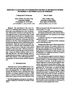
3.A MANUFACTURING RESOURCE UTILIZATION MODEL Our first step was to divide the activities in a manufacturing plant into three generic subactivities: manufacture of commodities, acquisition of new capital, and technical improvements to existing capital, as in the figure below. These subactivities were each represented as linear relations between quantities of inputs and of output, i.e. as Leontief production functions [8]. While fairly simple, these Leontief functions were sufficient to reproduce our planning manager’s reasoning. The most important process is the manufacture of final product. The elements of the input vector, IQ, are machine-hours, floor-space-hours, materials-spending and man-hours; they are linearly related to output, Q, subject to capacity constraint, C, by the relations of equation 1, where a is the vector of resource-per-unitrequirements.

I, = a * Q , Q < C

(11

Growth and technical change are represented as‘two separate processes, outside the production process, for two reasons. First, they are not necessary for output; a factory can produce products without process improvements, but not without raw materials. Second, they produce not material outputs but changes in the parameters of the production process. Technical change alters the a-vector; growth alters the capacity constraint. Below is the equation for technical change. It is linear in the percent improvement, and in the amount of equipment improved: la = # *I (C * Aai/ai) (2) In the equation for capital growth, AC is the change in capacity, and ICis a vector with elements of indirect labor for design and installation, and direct capital costs:

(3) I, = y * (AC) Equations were also added for cost-accounting, measuring performance, and miscellaneousrelations

4

The manufacturing, growth, and change models like volume discounting of purchases, increased pay for overtime, the learning-curve effects on productivity, and so on. In effect, these were a financial scaffolding built on top of a three-part physical model. The above three equations bring up a difficult, fundamental question: since the parameter values did not explicitly appear in'the plans, how could we get numerical values for the parameter vectors a, 8, y? Our answer comes from the observation that these values embody expertise in mlich the same sense that rule-strengthsembody expertise in rule-based expert systems. This analogy suggests that they might be elicited directly. Or, they might be estimated statistically from data, such as past history or the current plan. Estimation from historical data might reveal, for example, that the current plan assumes unusual productivity over its entire span. Estimation from the current plan might reveal outliers. In our case, however, the estimation process was trivial. Taking a cue from our human reviewer, we simply used values of parameters taken from current plant operations, which were readily available. Of course these would be quite unsuitable ifwe tried to use them to generate resource projections, since they would not take into account the characteristics of the products and manufacturing process being projected. However, for purposes of comparison, they provided the kinds of ballpark estimates that human reviewers used.

5

4. QUA NTlTATl VE REASON ING Given the set of equations and parameter values just described, the linkage between properties initially represented by rules can now be made by arithmetic operations on variables. In particular, it is now possible to determine the influence of variables on each other by tracing through the graph of relationships induced by the equations. However, since the human reviewer was only concerned with the most significant influences, it is important to be able to disregard "insignificant" effects during the reasoning process. To do that, we have developed a numeric influence measure called E which tells how much a set of variables effects a given variable, in the change between two contexts. If A = F(B,C),and the two contexts are 1 and 2, with A, = F(B,,C,) and A, = F(B,,C,), then 6's effect on A is defined by equation 4.

-

&(A,@)) = F(B,,c,) F(B,,C,) Likewise, the effect of both variables, (8C}, is defined by equation 5:

(4)

(5) E(A,{B C>)= F(B,,C.J - F(B,,C,) The two contexts could be two different years of a plan, or actual versus goal, or any other pair of contexts for which the variables were all related by the same F. To drop insignificant effects, and also allow for competing effects, we did not require a perfect match between E and the the change in A, AA. Rather, we said that a set X accounted for A A if inequality (6) held, where 7 was empirically set at 0.8. 1/7 > &(A,X)/AA > 7 (6) Unlike correlation coefficients, this measure is still accurate for nonlinear functional relationships. Unlike partial derivatives, it does not presume that other variables remain constant in determining the influence of a given variable. The slack in (6) also allows minor estimation inaccuracies to pass unnoticed. Further details may be found in Kosy & Wise [6].

A procedure for using this measure that matches the planning manager's review strategy can be stated as follows. Given a property of one variable, start tracing back, breadth first, via all equations involving that variable, collecting the influences that account for the property, until an "adequate cause" is found. If the tracing requires checking a variable whose value is not shown on the plan, find a suitable surrogate, and check it, where a surrogate is a variable whose value is shown that is functionally related to the missing variable. If a cause is found, but the relevant variable is not shown on the plan, check to make sure that its other expected effects, beside the initial property, are present.

One additional kind of knowledge must be included in a model in order to use this procedure to find an "adequate cause" of observed properties. A list of equations is not inherently directional, but causality is. Hence it is necessary to provide an ordering on the variables that indicates their precedence. This precedence was implemented by labeling equations as 'aggregation', 'definition', 'policy', or 'physical constraint'. An example aggregation would be the relation between total productivity and the various factor productivities, or between total labor and each sub-type of labor. An example definition would be that total productivity is the amount of output over the total value of all inputs. An example policy would be that inventory should be 20% of the yearly output, or that productivity should improve according to a learning curve with a pre-planned rate of improvement. Each of the three basic manufacturing plant processes are 'physical constraints'. The 'aggregation' and 'definition' labels serve as flags to make sure that the superordinate variable is explained in terms of the subordinate variables, not vice versa. If a variable is connected to a 'policy' equation, there is

6 no need to go beyond, because one or another of the variables in such an equation must be controllable (in order that the policy be implementable), and hence can be stopped at. Finally, to identify the end of a causal chain, certain variables were labeled as exogenous. No attempt is made to find causes for properties of these variables since they are taken to be outside the system being modeled. As a very simple illustration of how this procedure reproduces the planning manager's reasoning, consider the rule if employee-hours up, then expect material-spending u p and output up. Once "employee-hours up" has been noticed, that is traced to the exogenous variable, Q. However, no variable in the plan shows the value of Q in terms of volume of output produced. Rather, what is shown is the dollar volume of output, which is related to Q by price. Hence, the procedure checks the dollar output variable and, as a double-check, the other inputs (e.g., material-spending) required to produce plant output are also checked. A more complex example is if total-space up, employee-hours constanf, and distribution-space constant, then expect production-space up, output up, and capital-for-operafions-improvement positive. First, since total-space is defined as the sum of production-space and distribution-space,

then the total rising with distribution-spaceconstant requires production-spaceto rise. Second, while one input factor (space) rose, others (employee-hours) have stayed constant, hence the a-vector must have changed, and so the trace would proceed to examine inputs to the technical change process. In the original rule-set, the presence or absence of countering effects had been reflected by using multiple rules, one for each combination of missing and countering effects. These were later incorporated into the "unless.." clauses. For example, if oufput rose, increases in each input were expected. If output rose and an input did not rise, then a change in the a-vector was sought, because that is the only remaining term in ai'Q = li. Because a's were not listed in the plan, expenditure for capital improvements was checked, because that was a reliable surrogate, and hence a good check for whether the expected countering effect was actually present. Thus, the elicited rule actually embodies two distinct analyses, which the above procedure reproduces in sequence. Clearly the graph-searchingstrategy can trace whatever combinations are present, without needing a special rule for each one. However, one should note that this procedure is not exactly the same thing as what the manager described. That is, when asked how he reviewed resource plans, he gave many specific rules. Our general procedure traces influences, and mentions in sequence those variables that appear on the plan as it encounters them in the equational model. These turn out to be the same variables that the planning manager mentions in his rules. Our quantitative approach to explaining numerical results contrasts strongly, and instructively, with that of Bouwman [1,2]. Bouwman's domain was also quantitative data about a manufacturing concern, but the reasoning was performed.entirely in QA. His system basically scans the data, and, for each equation in the model, forms an expectation about the term it defines. For example, if A = B + C, B rose, and C rose, then A is expected to rise also. These expectations were then fitted together into chains, and those confirmed by the data were cited as explanations, discarding those contradicted by the data or simply not addressed by it. Our approach differs in that it begins at a variable and works out from there, rather than doing a complete scan before putting the pieces together. More importantly, Bouwman did not include cases where QA gives ambiguous results. While this strategy does prevent domination by (?)Is, it also rules out more accurate analyses when

7 the numbers are available. For example, if A depends mainly on B and C, but only slightly on D, then our significance test will detect that and not follow D.Q A would consider D to be just as important as 8 and C, unless D were omitted from the equation entirely. But then, it would be misled in those cases where D actually was important. Thus, Bouwman's approach is more dependent on a powerful and parsimonious model of a firm than is ours. It relies on the significant factors to have already been picked out when the model was specified, as it has no means of picking them out on a case-by-case basis. In the resource plans we examined, however, the relative magnitudes of the variables were crucial in deciding which lower level variables to explore next. In summary, we discovered that the original sixty-odd highly specific rules could be generated by general knowledge about arithmetic applied repeatedly, in different ways, to a more or less generic model of how resource variables are related in a manufacturing plant, as expressed by simple equations. This is in marked contrast to a system like MYCIN, where rules express empirical correlation but are not linked to a model. The use of arithmetic contrasts with a system like Bouwman's, which reasons purely qualitatively, not quantitatively.

5. THE REMUS EVALUATION PROCEDURE A version of the model and reasoning procedure just described has been adapted for use in the REMUS module of the ROME system[7]. ROME is an experimentaldecision support system generator that allows specification of planning models in terms of variables and algebraic formulas. Models may be executed and the results displayed in spreadsheet form. The purpose of REMUS is to Review and -Evaluate a Model's Underlying Structure by comparing results to evaluation criteria. Generic models-such as the one for manufacturing resource utilizatiorr-and quantitative reasoning are used to support the evaluation process.

Two sorts of evaluation criteria may be declared: norms and goals. A norm is a relationship among variables that "should" hold true under "normal" circumstances according to experts in the domain of the model. A goal is a statment of an organizational objective or policy that is likewise expressible in terms of model variables. Norms and goals are declared in ROME by expect and want statements, respectively. To illustrate, the three production functions in the manufacturing model are relationships that should hold true in a manufacturing plant. Expanding out the vectors in equation 1, and using somewhat more mnemonic variable names, yields the following set of norms: Expect Expect Expect Expect Expect

D i r e c t Labor Hours t o e q u a l Labor H o u r s I U n i t Q-produced T o t a l M a t e r i a l s Cost t o e q u a l M a t e r i a l $ / U n i t Q-produced T o t a l Floorspace Hours t o equal Floorspace H o u r s I U n i t Q-produced Q-produced T o t a l Machine Hours t o e q u a l Machine Hours/Unit Q-produced t o be no more t h a n P l a n t C a p a c i t y

Equation 2 has two components which may be expressed as follows: Expect abs(Xchange(Lab0r H o u r s / U n i t ( y ) ) ) t o equal P r o j e c t Hours(y-1) / Plant Capacity(y) Labor Hours p e r U n i t P r o d u c t i v i t y Change(y-1) Expect Xchange(Labor H o u r s / U n i t ( y ) ) t o equal Addon C a p i t a l Expense ( y - 1 ) / P l a n t C a p a c i t y ( y ) * C a p i t a l Cost p e r U n i t P r o d u c t i v i t y Change(y-1)

Equation 3 may be expressed similarly. Regarding goals, there may of course be many for a particular plant at a particular time. However,

8 there are two that tend to apply generically to manufacturing resource plans. The first is that new products should be manufactured more'efficientty than comparable current products, or at least no less efficiently. This goal, applied to labor efficiency, may be expressed to ROME as: D e c l a r e comparable p r o d u c t t o be an anchor v a r i a b l e D e c l a r e c u r r e n t year t o be a column v a r i a b l e We want Labor Hours/Unit t o be no more than Labor Hours/Unit f o r a comparable p r o d u c t i n t h e c u r r e n t year

The second goal is that productivity should improve at a desired rate as a function of the amount of production experience that has accumulated for a given product. This relationship is known as a 'learning curve', and one way to state the goal is: D e f i n e Cumulated-Q(y) t o be Cumulated-Q(y-1) + Q-produced(y) D e f i n e Cumulated D i r e c t Labor Hours(y) t o be Cumulated D i r e c t Labor Hours(y-1) + D i r e c t Labor Hours(y) D e c l a r e y l t o be a column v a r i a b l e Define y l t o be t h e f i r s t y e a r o f p r o d u c t i o n o f t h e product L e t Cumulated-Q(y1-1) = 0 L e t Cumulated D i r e c t Labor Hours(y1-1) = 0 D e f i n e % A d d i t i o n a l - Q ( y ) t o be Cumulated-Q(y) / Q-produced(y1) D e f i n e LCRF t o be t h e d e s i r e d l e a r n i n g curve c o s t r e d u c t i o n f a c t o r D e f i n e Alpha t o be logZ(LCRF) We want D i r e c t Labor Hours(y) t o be no more t h a n % A d d i t i o n a l - Q ( y ) ? Alpha Labor H o u r s / U n i t ( y l ) Cumulated-Q(y) - Cumulated D i r e c t Labor Hours(y-1)

To actually check these goals, their parameter values (e.g., comparable product, current year, LCRF) must be set. We will do this in a moment. The main steps in the REMUS evaluation procedure that applies the above criteria are shown below. To evaluate a variable v: 1. If there are criteria for the values of v , apply them and state conclusions.

Check equalities before inequalities. 2. Find variables that explain the trend in v using the formula for v given in the planning model. If there is no formula but there is an equality norm in the generic model, use that. Call this set of variables S. 3. If there are other variables in the formula which have evaluation criteria but are not in SI add them to S. 4. Recursively evaluate the variables in S. 5. Ifthere is no formula for v (S is empty), go on the the next variable to be evaluated. This procedure may be continued until it reaches exogenous variables. The main conclusions that may be drawn are as follows: 1. If criteria are met, say so. 2. If a goal is not met, conclude that Y is 'problematic'. 3. If there is a moderate difference (< 30%) between a value and a norm, conclude that v is 'OK' with respect to that norm. 4. If there is a large (> 30%) difference between a value and a goal, it is 'extraordinary'. If there is a large deviation from a norm, it is 'odd'. 5. If the effect on v of a large deviation in a lower level variable can be determined, suggest that v may be 'too high' or 'too low'.

The boundary between moderate and large differences is taken from Bouwman [l].

9 This procedure differs from the one described in the previous section in several respects. First, criteria are applied whenever possible. This tends to focus attention on every issue that may affect the top level variable being evaluated. Second, all explanatory variables are found at once, using the E measure and test 6. This contrasts with the hypothesize / check assumptions / find countering factor strategy. Moreover, explanation paths are pursued depth first, rather than breadth first. Both of these make it easier to express each step of the evaluation in words. Finally, REMUS makes no default assumptions about the values of variables not shown on a plan. Rather, these assumptions must be stated explicitly, if needed. The reason for this is to make sure the user knows what assumptions are being used, and to sidestep the problem of choosing good surrogate variables. One thing remains to be done before we can use this procedure to evaluate a specific resource plan and that is to link the criteria to the particular variables in that plan. Consider the portion of a resource plan shown below:

- -_--------__----_redWood===:==:==== -

1985===t1986====1987==:=1988====1989====1990

p r o d u c t i o n spending 1.40 0.0 mfg d l S other dl $ 1.37 mfg employee-hours 0.0 o t h e r employee-hours 31.40 labor r a t e 44.47 process improvement h r s 0 . 0 c a p i t a l f o r improvement 0 . 0 o u t p u t SM 0.0 avg p r i c e

4.87 2.49 2.38 44.40 42.50 56.00 0.0 0.0 36.75 .25

4.79 4.08 .71 73.60 12.80 55.44 0.0 0.0 62.16 .21

3.45 2.86 .58 50.79 10.30 56.38 0.0 0.0 52.06 .19

4.73 3.90 .82 62.68 13.20 62.27 0.0 0.0 65.36 .19

5.85 4.94 .92 77.21 14.40 64.02 0.0 0.0 81.13 .19

--_--_-------------_-----_------- -----

----_-----------_--_c____________

"Redwood" is the name of a new product that is to be introduced in 1986. The relationships in the planning model that generated these results are as follows: D e f i n e p r o d u c t i o n spending t o b e mfg d l $ + o t h e r d l S E s t i m a t e mfg d l $ t o be mfg employee-hours l a b o r r a t e / 1000 E s t i m a t e o t h e r d l $ t o be o t h e r employee-hours * l a b o r r a t e / 1000

All the other values are input. Dollar values are expressed in millions except for labor rate, and labor hours are expressed in thousands.

The variables in this plan may be linked to variables in the generic model given above by declaring them to be "kinds" or "measures" of the corresponding generic variables. The norms and goals from the generic model will then become norms and goals for the planning variables by a process of "inheritance" described in [7]. The ROME statements expressing these correspondences are: D e c l a r e mfg employee-hours t o b e a k i n d of D i r e c t Labor Hours D e c l a r e c a p i t a l f o r improvement t o be a k i n d o f Addon C a p i t a l Expense D e c l a r e process improvement h r s t o be a k i n d of P r o j e c t Hours Assume Q-produced t o e q u a l o u t p u t SM / avg p r i c e D e c l a r e l a b o r r a t e , Labor H o u r s / U n i t and Q-produced t o be exogenous D e f i n e Labor Hours/Unit t o be D i r e c t Labor Hours / Q-produced

Several other facts that bear on the evaluation are also known. The current product being produced in 1985 is called "Hemlock" and the labor needed to manufacture it is 640 hourshnit. For the new product, Redwood, being introduced in 1986, it is desired that productivity improve by 10% for each doubling in cumulative output. The production process for Redwood will be similar to that for Hemlock. This information can be stated as follows: D e f i n e c u r r e n t y e a r t o be 1985 L e t Labor Hours/Unit(hemlock,l985)

= .64

10

L e t comparable product(redwood) = hemlock D e f i n e yl(redwood) t o be 1986 We want LCRF(redwood) t o be . 9 L e t Labor Hours per U n i t P r o d u c t i v i t y Change(redwood) = Labor Hours per U n i t P r o d u c t i v i t y Change(hem1ock) L e t C a p i t a l Cost p e r U n i t P r o d u c t i v i t y Change(redwood) = C a p i t a l Cost per U n i t P r o d u c t i v i t y Change(hem1ock) L e t P l a n t Capacity(redwood) = P l a n t Capacity(hem1ock)

We are now in a position to evaluate several variables in the plan. However, we will only show the evaluation for one -- production spending -- since the others will be evaluated along the way:

> E v a l u a t e p r o d u c t i o n spending(redwood) f o r 1989 There are no e v a l u a t i o n c r i t e r i a f o r p r o d u c t i o n spending(redwood) i n 1989. However, redwood p r o d u c t i o n spending goes up i n 1989 because mfg d l $ and o t h e r d l $ b o t h go up and p r o d u c t i o n spending mfg d l $ + o t h e r d l $ . The i n c r e a s e i n p r o d u c t i o n spending was due p r i m a r i l y t o t h e i n c r e a s e i n mfg d l $. Would you l i k e me t o continue? Y Redwood m f g d l $ goes up i n 1989 because mfg employee-hours and l a b o r r a t e b o t h go up l a b o r r a t e / 1000. The i n c r e a s e i n mfg d l $ was and mfg d l $ = mfg employee-hours due p r i m a r i l y t o t h e i n c r e a s e i n mfg employee-hours. Would you l i k e me t o c o n t i n u e ? Y By norm 1, we expect redwood mfg employee-hours t o equal Labor H o u r s / U n i t Q-produced. Assuming Q-produced = o u t p u t $M / avg p r i c e , t h i s appears t o be so i n 1989. By g o a l 2 , we want redwood mfg employee-hours t o be no more than Cumulated-Q(y) % A d d i t i o n a l - Q ( y ) t Alpha Labor H o u r s / U n i t ( y l ) Cumulated D i r e c t Labor Hours(y-1). T h i s appears t o be so i n 1989. B u t we a l s o f i n d redwood mfg employee-hours t o be much l e s s than t h a t v a l u e i n t h a t y e a r . T h i s seems e x t r a o r d i n a r y . So redwood mfg employee-hours may be t o o low i n 1989. which means mfg d l $ may be t o o low. which means p r o d u c t i o n spending may be t o o low. Would you l i k e me t o c o n t i n u e ? Y

-

By norm 6, we expect abs(%change(redwood Labor H o u r s / U n i t ( y ) ) ) t o equal process improvement h r s ( y - 1 ) / P l a n t C a p a c i t y ( y ) * Labor Hours p e r U n i t P r o d u c t i v i t y Change(y-1). T h i s seems t o be OK i n 1989. By norm 7 . we expect Xchange(redwood Labor H o u r s / U n i t ( y ) ) t o equal c a p i t a l f o r C a p i t a l Cost p e r U n i t P r o d u c t i v i t y Change(y-1). improvement(y-1) / P l a n t C a p a c i t y ( y ) T h i s seems t o be OK i n 1989. By g o a l 1, we want redwood Labor H o u r s / U n i t t.0 be no more t h a n Labor Hours/Unlt (hemlock.1985). T h i s appears t o be so i n 1989. B u t we a l s o f i n d redwood Labor H o u r s / U n i t t o be much l e s s t h a n t h a t v a l u e i n t h a t y e a r . T h i s seems e x t r a o r d i n a r y . So, again, mfg employee-hours may be t o o l o w i n 1989, which means mfg d l $ may be t o o low, which means p r o d u c t i o n spending may be t o o l o w . Would you l i k e me t o c o n t i n u e ?

The procedure would now go on to evaluate Q-produced, labor rate, and other dl $. It can be seen from the above, however, that the 1989 projection for mfg employee-hours is quite optimistic. This, in turn, diminishes the credibility of the mfg dl $ and production spending values that depend on it.

6. CONCLUSIONS Evaluating a resource plan may be viewed as a process by which a reviewer compares what he knows or believes to what he is told by the numbers in a plan. For a computer program to perform such comparisons, it must use some representation of a reviewer’s knowledge and beliefs. While our initial representation of this knowledge was in terms of if-then rules, we discovered that relatively simple linear-equation models could be used to encode the same information at a more fundamental, structural level. We also developed an algorithm for exploring equational models, and the influence measure necessary to make quantitative, but still approximate, inferences from them.

11

Although, in this paper, we have confined our attention to evaluating resource plans, the issues involved are very much related to the 'general problem of model validation. Hence, it may not be surprising that parts of the evaluation strategy we induced from a human reviewer's protocols are similar to more formal model validation techniques. For example, in hypothesizing variables that should change when a change is observed in a given variable, a human reviewer is performing a kind of sensitivity test. In comparing the value of a variable against what that value would be for current plant operations, he is essentially trying to verify that the planning model would produce correct results for a known test case. Finally, the entire strategy rests on the principle that values can best be judged by comparing them to other values that have independent justification. The chief strength of the REMUS procedure is that it allows evaluation of a result even if there are no criteria directly applicable to it. By descending to subordinate variables that affect a given variable, this procedure conducts a search for criteria that may be relevant based on functional relationships. Moreover, because the variables in a given planning model can be linked to expected relationships, a given set of criteria can be transferred to other models in the same domain. Together, these mechanisms provide a means of using relatively general, structural models to make judgments about specific cases.

REFERENCES Bouwman, M.J., Financial Diagnosis: A Cognitive Model of the Processes Involved, PhD Thesis, Graduate School of Industrial Administration, Carnegie-Mellon University, 1978. Bouwman, M.J., "Human Diagnostic Reasoning by Computer: An Illustration from Financial Analysis," Management Science, V. 29,No. 6,pp. 653-672, June 1983. Davis, R., Applications of Meta Level Knowledge to the Construction. Maintenance and Use of Large Knowledge Bases, PhD Thesis, Computer Science Department, Stanford University, July

1976. Doyle, J., "Methodological Simplicity in Expert System Construction: Judgments and Reasoned Assumptions," The AI Magazine, V. 4, No. 2, pp. 39-43, Summer 1983. Kosy, D.W., and Dahr, V., "Knowledge-Based Support Systems for Long Range Planning," The Robotics Institute, Carnegie-MellonUniversity, 1983. Kosy, D.W., and Wise, B.P., "Self-Explanatory Financial Planning Models," Proceedings of AAAI-84, pp. 176-181, August 1984.

Kosy, D.W., and Wise, B.P., "Overview of ROME: A Reason-Oriented Modeling Environment," The Robotics Institute, Carnegie-MellonUniversity, 1985. Leontief, W., et al., Studies in the Structure of the American Economy, New York: Oxford University Press, 1954. McDermott, J., "Rl: A Rule-Based Configurer of Computer Systems," Artifial Intelligence, V. 19,

No. 1 , pp. 39-88,September 1982.