Model-Based Geostatistics the Easy Way - Journal of Statistical Software

JSS

Journal of Statistical Software January 2015, Volume 63, Issue 12.

http://www.jstatsoft.org/

Model-Based Geostatistics the Easy Way Patrick E. Brown Cancer Care Ontario and University of Toronto

Abstract This paper briefly describes geostatistical models for Gaussian and non-Gaussian data and demonstrates the geostatsp and dieasemapping packages for performing inference using these models. Making use of R’s spatial data types, and raster objects in particular, makes spatial analyses using geostatistical models simple and convenient. Examples using real data are shown for Gaussian spatial data, binomially distributed spatial data, a logGaussian Cox process, and an area-level model for case counts.

Keywords: spatial statistics, geostatistics, R, INLA, Bayesian inference, kriging.

1. Introduction In the past two decades spatial statistics has gradually become a mature and established branch of statistics with a suite of well defined models and proven inference methodologies capable of addressing a wide range of practical problems. The capability of R (R Core Team 2014) to store, manipulate, and display spatial data has similarly improved, and as a result spatial methodologies which were formerly only accessible to the specialist are available to the wider statistical community. This paper demonstrates model fitting for Gaussian, nonGaussian, and point process data using the geostatsp and diseasemapping packages, with R’s spatial data classes being used to make spatial data analysis simple and the software intuitive.

1.1. Models and methods Models and theory for Gaussian spatial data were first espoused by Matheron (1962) and popularized by Cressie (1993). Writing U (s) as the value of a Gaussian random field U at location s, the basic (stationary) geostatistical model is characterized by the joint multivariate normal distribution [U (s1 ) . . . U (sN )]> ∼ MVN(0, Σ).

2

Model-Based Geostatistics the Easy Way

The entries of the covariance matrix Σ are determined by a spatial correlation function ρ with Σij = cov[U (si ), U (sj )] = σ 2 ρ[(si − sj )/φ, θ]. Here φ is a scale parameter controlling the rate at which correlation decays with distance, and θ is a vector of possible additional parameters (controlling directional effects, for example). An isotropic process has correlation being a function of distance with ρ[(si −sj )/φ] = ρ0 (||si − sj ||/φ). Various parametric functions have been used for ρ, and Stein (1999) makes a compelling case for the Mat´ern correlation function described in Appendix A. An isotropic process with a Mat´ern correlation has a single additional parameter κ controlling the differentiability of the process. Two additional covariance parameters commonly used refer to geometric anisotropy, and comprise an angle of rotation indicating a preferred direction and a ratio parameter giving the ratio of the ranges on the two axes. The parametrisation of the Mat´ern is different in each of the geoR (Ribeiro and Diggle 2001), RandomFields (Schlather, Malinowski, Menck, Oesting, and Strokorb 2015) and geostatsp packages. The specification of the Mat´ern in Appendix A, and in use in the geostatsp package, has the property that when varying κ the correlation at a distance φ stays fairly close to 0.14, or ρ[(0, φ)/φ, κ] ≈ 0.14. A Mat´ern with κ = ∞ is a Gaussian density with φ being two standard deviations. The term ‘practical range’ is used at times to describe φ as defined here, interpreting φ as a distance beyond which correlation is ‘small’ is a manner analogous to interpreting the Gaussian density as being ‘small’ beyond two standard deviations. The anisotropy angle refers to rotation of the coordinates anti-clockwise by the specified amount prior to calculating distances, which has the effect that the contours of the correlation function appear rotated clockwise by this amount. The anisotropy ratio is the amount the Y coordinates are divided by by following rotation, with large values making the Y coordinates smaller and increasing the correlation in the Y direction (of the rotated coordinates).

Gaussian data Data Yi observed at location si with covariates X(si ) is often modelled with the linear geostatistical model (LGM): Yi |U (si ) ∼N(λ(si ), τ 2 ) λ(si ) =µ + βX(si ) + U (si ).

(1)

Although method-of-moments estimation of the covariance parameters φ, σ and τ is still common, Stein (1999) makes a thorough argument for using maximum likelihood estimates (MLEs). Writing ψ = (µ, β, σ, τ, φ), the MLEs ψˆ are the quantities which maximize the likelihood pr(Y1 . . . YN ; ψ). The Yi are jointly multivariate normal and the likelihood is tractable, albeit requiring the inversion of an N by N matrix, and numerical optimizers such as the ˆ optim function can be used to find ψ. Spatial prediction usually involves covering the study region with a large number of reg¯ = [U (g1 ) . . . U (gL )] or ularly spaced points g` ; ` = 1 . . . L and mapping estimates of U ¯ ¯ |Y ] λ = [λ(g1 ) . . . λ(gL )]. As the model is linear and Gaussian, the conditional distribution [U is multivariate normal with closed form expressions for the conditional mean and variance. The MLEs ψˆ are used to calculate these expressions, hence the uncertainty in these parameter estimates is ignored (see Diggle and Ribeiro 2006).

Journal of Statistical Software

3

Non-Gaussian data When the observed data Yi are non-Gaussian, the model above is extended to the generalized linear geostatistical model (GLGM) used by Diggle, Moyeed, and Tawn (1998) and further described in Diggle and Ribeiro (2006). Consider a distribution f (i.e., Binomial or Weibull) with a mean parameter λ and possibly additional parameters ν. Writing g(·) as a link function (i.e., log or logit), the GLGM takes the form Yi |U (si ) ∼f [λ(si ), ν] g[λ(si )] =µ + βX(si ) + U (si )

(2)

cov[U (si ), U (sj )] =σ 2 ρ[(si − sj )/φ, θ]. The combination of non-Gaussian data and an unobserved latent variable make the likelihood function intractable and computing the MLEs difficult. Bayesian inference using Markov chain Monte Carlo (MCMC) algorithms has become the most common method for making statistical inference with GLGMs, as was done in Diggle et al. (1998). Bayesian inference requires specifying prior distributions for the model parameters µ, β, σ and φ, with the posterior distributions π(φ|Y ) and π[U (s)|Y ] forming the basis of inference. The integrated nested Laplace approximation (INLA) algorithm of Rue, Martino, and Chopin (2009) is an alternative to MCMC for performing Bayesian with latent Gaussian models. MCMC’s principal drawback is the requirement that chains of posterior samples must be monitored and assessed for convergence and mixing, and obtaining a set of reliable posterior samples from a MCMC algorithm can be difficult and require a specialized skill set to accomplish. INLA is much easier to use in this regard, and although it’s maximisation step and numerical integration can sometimes require judicious choices of starting values and tuning parameters it is in general less labor-intensive to use than MCMC. An additional recent development which has facilitated the implementation of the GLGM is the Markov random field approximation to the Mat´ern correlation function developed by Lindgren, Rue, and Lindstr¨ om (2011). When the number of spatial locations N is large, inverting the variance matrix Σ can be time consuming or numerically unstable. Lindgren et al. (2011) use Gaussian Markov random fields (GMRF’s) to derive a simple expression for Σ−1 for Mat´ern correlations using various forms of stochastic partial differential equations. The geostatsp package makes use of the Mat´ern approximation of GMRF’s on grids of square cells with κ = 1 or 2. Although real datasets will rarely be sampled on a square lattice, the continuous surface U (s) can be well approximated by superimposing a fine lattice over the study region and assigning each data point to a cell. The fact that many (or most) of the cells will not have data observed in them is not problematic for INLA. This combination of INLA with the Markov random field approximation has been to estimate spatial variation in risk for Lupus in the city of Toronto, Canada from case incident locations by Li, Brown, Rue, al Maini, and Fortin (2012), and for assessing the effect of cancer risk of ambient radiation near a nuclear power facility using time-to-event data from a retrospective cohort in Jiang, Brown, Rue, and Shimakura (2014). Lindgren et al. (2011) derive a GMRF approximation for the Mat´ern using an irregular lattice with triangular basis functions, which has a number of advantages over the grid cell approach. This approximation is implemented in the INLA software, and incorporation of this feature into geostatsp is work in progress.

4

Model-Based Geostatistics the Easy Way

1.2. Spatial statistics and R The sp package (see Bivand, Pebesma, and G´omez-Rubio 2013) and raster package (Hijmans 2014) provide an excellent set of facilities for storing, manipulating, and visualising spatial data. The sp package provides SpatialPointsDataFrame and SpatialPolygonsDataFrame objects for storing point and polygon data respectively, and are compatible with many of the standard data formats most geographical information systems (GIS) uses. The raster package provides similar tools for raster data, which are pixelated images or rectangular lattices. The rgdal (Bivand, Keitt, and Rowlingson 2014) package provides a set of tools for reading spatial data from various formats into R, such as ESRI shapefiles for point and polygon data, and GeoTIFF files for raster data. These three packages (along with spdep, Bivand 2014, and others) have made R fully compatible with GIS software and R fulfils many of the criteria for it to be called a GIS in its own right. The venerable geoR package (see Diggle and Ribeiro 2006) has provided tools for likelihoodbased inference since 2000, and is one of the very few software packages for spatial analysis which accommodates all of: the Mat´ern correlation function; covariates; Maximum Likelihood Estimation; geometric anisotropy; and the Box-Cox transform. Since geoR predates the sp and raster packages, it has its own spatial data types. For Bayesian inference, the excellent INLA (Rue, Martino, Lindgren, Simpson, and Riebler 2013) package developed by the authors of Rue et al. (2009) and Lindgren et al. (2011) implements INLA for a wide variety of models, including spatial Gaussian Markov random field models. INLA has been designed with flexibility of model specification being a priority, a job INLA accomplishes to an astonishing degree albeit at the cost rendering some tasks relatively complex in comparison to other packages. One such example is specifying a Mat´ern correlation function, with spatial locations being specified as grid cell indexes rather than coordinates. A considerable amount of code can sometimes be necessary for converting INLA results from a spatial model into a format which can be mapped. The geostatsp package provides a set of user-friendly functions for Gaussian spatial models and an easy interface to INLA for fitting non-Gaussian models, resulting in a powerful set of tools for model-based geostatistical analyses in R. Response variables and covariates are specified with formulas, with data provided as Raster or SpatialPointsDataFrame objects. The interface to INLA has more complex set of routines underlying it, with observations being allocated to cells in a Markov random field and linear combinations of parameters and latent variables for predicted spatial surfaces being defined. The spatial predictions obtained from these packages are raster objects, making them easy to display and overlay on background maps.

2. Model-based geostatistics through examples The geostatsp and diseasemapping packages described in this paper are available from the Comprehensive R Archive Network at http://CRAN.R-project.org/ and R-Forge at http: //R-Forge.R-project.org/R/?group_id=312. They both depend on the INLA package obtainable from http://R-INLA.org/.

Journal of Statistical Software

5 rain(mm)

●●

● ● ● ● ● ● ●

● ●

●

●

●●

●

●● ● ● ● ●● ● ●● ● ● ● ● ● ● ● ●● ● ● ● ● ● ● ● ● ● ● ● ● ● ● ● ● ● ● ● ● ● ● ● ● ● ● ●● ● ● ● ● ● ●● ● ● ● ● ● ● ● ● ●● ● ● ● ● ● ● ● ● ● ● ● ● ● ●

●

● ●

●

60 30 20 10 0

elevation(m) 5000 4000 3000 2000 1000 0

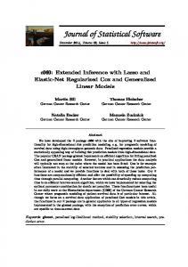
Figure 1: Swiss rainfall data (colored blue points and top legend) with elevation (background colors and bottom legend).

2.1. Maximum likelihood estimation and kriging The Swiss rainfall dataset (see Diggle and Ribeiro 2006, 5.4.7) is a classic case study in Gaussian geostatistics. Loading of the geostatsp package and executing data("swissRain") makes available the following objects: a SpatialPointsDataFrame named swissRain of rain values at a number of points, a SpatialPolygonsDataFrame named swissBorder of the border of Switzerland; and a Raster object swissAltitude containing elevation values for Switzerland. These three objects are plotted in Figure 1. Using the linear geostatistical model in (1) with these data would have the rainfall measurements being the Yi , elevation values being X(s), and λ(s) as the unknown true rainfall surface. Either Bayesian or Frequentist inference could be used to fit the model, with the former possible in a manner similar to the example in the subsequent section. Frequentist inference is accomplished with the lgm function in the geostatsp package, which in turn calls likfitLgm for estimating the model parameters and krige for computing conditional means and variances of U (s) and λ(s). The Swiss rainfall data is fit with the code below. R> names(swissRain) [1] "ID"

"rain"

R> names(swissAltitude) [1] "CHE_alt" R> swissFit names(swissFit)

6

Model-Based Geostatistics the Easy Way

(Intercept) Elev’n per 1000m range, km sdNugget anisoAngleDegrees anisoRatio shape boxcox sdSpatial

Estimate 4.86 0.28 0.06 0.95 37.00 7.48 1.00 0.50 2.97

Std. error 1.29 0.37

CI 0.025 2.32 −0.45 0.03 0.73 31.74 3.94

CI 0.975 7.39 1.01 0.11 1.24 42.27 14.19

1.89

4.68

Estimated true true true true true true false false true

Table 1: Swiss rainfall parameter estimates, standard errors and confidence intervals obtained from a linear geostatistical model and the lgm function. [1] "predict" [5] "data"

"param" "model"

"varParam" "optim" "summary"

The data and covariates arguments contain the data required for fitting the model, with the fixed effects βX(s) specified by formula. The variables listed in formula refer to names in either the swissRain or swissAltitude objects, and are not the names of the objects themselves. Variables in the right hand side of formula can refer to either: the name of a vector of values contained in the data argument; the name of a layer in a Raster object (a single layer, brick or stack) passed as covariates; or the name of one of the elements if covariates is a list of Raster objects. The latter is useful when covariate rasters have different resolutions and projections. If a covariate is a column in data, it will not be included in the predicted values for λ(s). The argument grid = 120 specifies that spatial prediction should be done on a raster with 120 cells in the X dimension, with this raster having square cells covering the bounding box of swissRain. The grid argument can alternatively be supplied as a Raster object. A Mat´ern spatial correlation function with shape parameter fixed at 1 and a Box-Cox transform with parameter fixed at 0.5 (a square-root transform) are used. The aniso = TRUE argument allows for geometric anisotropy in the correlation function. Additional function arguments are param and parscale, starting values and parameter scaling values passed from lgm to likfitLgm and ultimately the numerical optimizer optim. The Swiss data has spatial locations expressed in a UTM projection, with coordinates in metres and consequently a spatial range parameter likely to be in the hundreds of thousands. The default scaling of 1 in optim would be ineffective and arguments on the order of param = c(range = 10^5) and parscale = c(range = 10^4) are in order. The default starting value and scale which likfitLgm sets for the range parameter are 1/20 and 1/200 of the diagonal distance of the bounding box of data. The swissFit object produced by lgm is a list with elements including predict, a RasterStack of spatial predictions and standard errors, and summary, a table of parameter estimates and confidence intervals. Table 1 shows the summary component, with the range parameter converted to kilometres. The standard deviation parameters σ and τ are displayed in the sdSpatial and sdNugget rows respectively. Confidence intervals for the covariance parameters are derived from the observed information matrix, and will be missing if any of the

Journal of Statistical Software

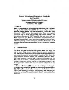
(a) Predicted rainfall E(λ(s)|Y )

7

(b) Exceedance probabilities pr(λ(s) > 30|Y )

Figure 2: Conditional expectations and probabilities obtaind from fitting a linear geostatistical model to the Swiss rainfall using the lgm function. estimated parameters are on a boundary. Notice the ‘Estimated’ column indicating that the Mat´ern shape parameter and Box-Cox transformation parameter were not estimated from the data. Spatial predictions of the rainfall surface λ(s) and the spatial random effect U (s) are contained in the RasterStack element of swissFit$predict, which has the following layers: R> names(swissFit$predict) [1] "space" [4] "krigeSd"

"random" "predict"

"predict.boxcox"

Using the notation in (1), these layes are (in the order given above): the predicted fixed effects ˆ µ ˆ + βX(s); the kriged random effects E[U (s)|Y ]; the predicted rainfall surface E[λ(s)|Y ] on the Box-Cox transformed scale; the prediction standard deviation sd[U (s)|Y ]; and predicted rainfall on the natural scale E{[αλ(s) + 1]1/α |Y } with α being the Box-Cox transformation parameter. Figure 2a shows the predicted rainfall values (on the natural scale), and results from the command plot(swissFit$predict[["predict"]]). Notice the strong directionality is consistent with an angle of rotation of 37◦ and a ratio of the major to minor axes of 7.5. Figure 2b shows the conditional probabilities that rainfall exceeds 30mm, computed with R> exc30 oneSim R> R> R> R> + + + +

swissRain$alt R> R> R> + R>

library("geoRglm") loaNoMissing R> R>

library("diseasemapping") data("kentucky") larynxRates R> R> + + + +

library("spdep") kAdjMat library("R2OpenBUGS") R> kResult + R> + R> + R>

covariates + R> R> +

Npoints