Model Based Macro-Editing Approach to State and Area Estimates ...

Model Based Macro-Editing Approach to State and Area Estimates from the Current Employment Statistics Survey1 Julie Gershunskaya U.S. Bureau of Labor Statistics, 2 Massachusetts Ave NE, Suite 4985, Washington, DC, 20212

Abstract Estimates of employment from the Current Employment Statistics (CES) survey are published every month for a large number of cells defined at various detailed industrial and geographic levels. Before the estimates are released for publication, they need to be reviewed. The purpose of the review is to isolate cells that may contain erroneously reported and influential records not captured during the editing procedure. The traditional approach to the macro-editing is to compare the current estimates to the historical data and mark any significant deviation as suspicious. However, it may happen that estimates deviate from the historical records for legitimate reasons (for example, due to a changing economic pattern). We propose to use a model based approach leading to a more effective screening. The model considered in this paper is the area-level Fay-Herriot model, where we apply a robust method for estimating the model parameters. A standardized difference between the sample based estimate and the synthetic part of the model predictor is used as the basis for screening. While the general CES policy is to rely on the purely sample based estimates when the sample is moderately large, a possibly useful by-product of the proposed screening procedure is the set of the robust modelbased estimates that can be used to replace the direct sample estimates in a limited number of extreme cases.

Key Words: statistical data editing, macro-editing, outlier, robust small area estimation

1. Introduction Before survey estimates produced by statistical agencies are released for publication, they need to be reviewed. Usually, the estimates are compared to analogous quantities from past years of the same survey. Large deviations from these quantities are deemed suspicious and are subjected to further analysis. A procedure for identifying unusual estimates is called the aggregation form of macro-editing. See more discussion in De Waal (2009). There are several drawbacks in the traditional aggregation method of macro screening: past quantities may deviate from the current estimates for legitimate reasons; the allowed amount of deviation from past quantities is somewhat arbitrary. The procedure may lead to biased estimates; “bending” current estimates in the direction of past years’ values may result in missed “turning points.”

1

Any opinions expressed in this paper are those of the author and do not constitute policy of the Bureau of Labor Statistics.

In this paper, we formalize the aggregation method of macro-editing in terms of a statistical model. This allows for the opportunity to apply standard methods of model fitting and checking in exploring deviations from the assumed model. The proposed method is based on the well-known Fay-Herriot model (Fay and Herriot 1979), which belongs to the area-level model variety employed in small area estimation (SAE). A distinguished characteristic of area-level models is that the area-level summary statistics (e.g., direct sample estimates) enter into a model as observed data. Auxiliary variables used in the model, as well, carry information at the area level. This makes arealevel models suitable for application for the aggregate type of macro-editing. The traditional past years’ quantities are now used as auxiliary variables in the model. Let Yˆi denote the sample based estimate in area i and let Di be its sampling variance.



Suppose a vector Xi  X i1 ,..., X ip



T

of auxiliary information is available for each area.

The Fay-Herriot model is given by conditions (1) and (2) below. For each area i  1,..., M ,

Yˆi ~ N Yi , Di  ,

(1)

Yi ~ N  XTi β, A  ,

(2)

ind

ind

where a p - dimensional vector of coefficients β and variance A are unknown parameters of the model, Yi is the unknown true population parameter, which is the target of the estimation. Variance Di is assumed to be known. In practice, some form of a generalized variance function is used to approximate variances. Suppose for a moment that parameters β and A are known. The screening idea is simple. Form standardized values

ri 

Yˆi  XTi β . Di  A

(3)

If the model holds, then ri ’s are independent standard normal variables: iid

ri ~ N  0,1

(4)

Then, for a pre-specified threshold h , the values Yˆi for which ri exceeds the threshold in absolute value ( ri  h ), are marked as outliers. There are two general reasons for extreme values in direct estimates. It may happen that a direct estimate does not estimate the finite population parameter well; for example, it may be due to a non-sampling error or it could be caused by gross errors in micro records. We call such an estimate a “real” outlier. We might say that assumption (1) does not hold for such an area. Another possibility is that, although Yˆi may be a reasonable estimate of the truth, assumption (2) does not hold for the true population parameter in area i . In such a

case, we would “falsely” mark the estimate Yˆi as an outlier. Thus, a follow up analysis of the screened estimates is important.

2. Robust estimation of the model parameters Existence of outliers points to a model failure. In other words, it contradicts the assumption that the model holds for all observations. Thus, we regard statements (1) and (2) as the working model, assuming it holds for the bulk of the data while allowing the possibility for extreme values in a handful of Yˆi ’s. Since parameters β and A are unknown, they have to be estimated from the data. To protect estimates of the model parameters from the effects caused by extreme values in

Yˆi ’s, we use a robust method of estimation based on bounded Huber functions. To estimate the parameters, Fay and Herriot (1979) solve simultaneously the following equations (5) and (6): M



Yˆ  X β  X Di  A

i 1

M



T i

i

Yˆ  X β  T i

i

Di  A

i 1

i

 0,

(5)

 M  p.

(6)

2

Instead of (5) and (6), let us solve corresponding robustified system of equations: M

 i 1

1  b  ri  Xi  0, Di  A

M

  r    M  p  E i 1

where ri 

Yˆi  XTi β Di  A

2 b

i



 b2  r   ,

(7)

(8)

and  b  ri  is a bounded function; E  b2  r   is expectation of

 b2  r  under standard normality of random variable r . The above equations are in analogy to Huber’s Proposal 2 (Huber 1964; see also Hampel et al. 1986, page 234.) If  b  ri  is the Huber function

 b  ri   min  b, max  b, ri   ,

(9)

for a predetermined fixed 0  b   , then

E  b2  r    2    b   1 1  b2   1  2b  b  ,

(10)

where    is the standard normal cumulative distribution function and and    is the standard normal probability density function. For example, if b  1.345 then

E  b2  r    0.7102 and if b  2 then E  b2  r    0.9205. In what follows, we denote E  b2  r   by letter c . To solve (7) and (8), we apply the Newton-Raphson algorithm and find zeros of the following functions f1  β  and f 2  A : M

1  b  ri  Xi , Di  A

(11)

f 2  A    b2  ri    M  p  c.

(12)

f1  β    i 1

M

i 1

The corresponding derivatives are

f1  β  M  b  ri  1  XTi , β β Di  A i 1

(13)

M f 2  A    r   2 b  ri  b i . A A i 1

(14)

The derivatives of  b  ri  are

 b  ri   b  ri  1  Xi , β Di  A ri

(15)

 b  ri   b  ri  1 1 ,  ri 2  Di  A  A ri

(16)

where, for the Huber function (9), we have

 b  ri  0,  I  ri  b   ri  1

ri  b ri  b

.

(17)

Thus, at the k-th step of the Newton-Raphson algorithm, we find M

 b  ri ,k 1  Xi Di  Ak 1 β k  β k 1  M , 1 T Xi Xi I ri ,k 1  b  i 1 Di  Ak 1



1

i 1





(18)

M

Ak  Ak 1 

  r    M  p  c m 1

2 b

i , k 1



M



1  b  ri ,k 1  ri ,k 1 I ri ,k 1  b  i 1  Di  Ak 1 

where ri , k 1 

Yˆi  XTi β k 1 Di  Ak 1

,

(19)

and subscripts k  1 and k signify estimated parameter

values at the respective steps of the algorithm.

3. Application to CES data 3.1 Previously used screening method and the proposed CES model Each month, CES sample reports are used to estimate relative change in employment for the continuous part of the population of businesses (that is, the set of establishments that have positive employment in both previous and current months). For estimation cell i at month t , this estimate is obtained as the ratio of two survey weighted sums

Rˆi ,t 

 

jSi ,t

jSi ,t

w j y j ,t

w j y j ,t 1

,

(20)

where y j ,t and y j ,t 1 are employment levels reported by a unit j at months t and t  1 ;

S j ,t is a set of reporting units that have positive employment in both adjacent months. To obtain the current month estimate of the level of employment in cell i , the estimate of the relative change Rˆi ,t is applied to the previous month estimated level of employment

Yˆi ,t 1 and a model-based net births-deaths factor, Nˆ i ,t , is added to the result: Yˆi ,t  Yˆi ,t 1 Rˆi ,t  Nˆ i ,t .

(21)

Adjustment Nˆ i ,t is a projected net difference of employment added by births and lost from deaths of businesses in cell i (see BLS Handbook of Methods 2004). The recursive scheme (21) originates once a year from a known level Yi ,t  0 that is available on a lagged basis from the quarterly census of employment. Let

Yˆ Tˆi ,t  i ,t Yˆi ,t 1

(22)

be the estimated relative change in employment level. It has long been observed that monthly changes in employment have a pronounced seasonal pattern, as well as industry and geography specific character. The assumption that current sample based estimates of the monthly changes should not substantially differ

from the corresponding historical values has always been used to screen for suspicious large deviations. The method considered in this paper is built on a similar belief. Namely, we assume that historical data correlate with the current estimates. The model based approach formalizes, refines and quantifies the old screening procedure. Auxiliary variable X i ,t is the relative change in employment at month t in cell i, as forecasted from the historical data. It is assumed that X i ,t is a good predictor of the true change Ti ,t . Consider a set of estimation cells i  1,..., M . For example, this may be a set of States within an industrial division. (In what follows, we call the elements of this set “areas”, as is customary in the SAE field.) Modeling assumptions (1) and (2) can be written as

Tˆi ,t ~ N Ti ,t , Di ,t  ,

(23)

Ti ,t ~ N   X i ,t , At  .

(24)

ind

We refer to the above model as Model 1. There is a certain belief that the monthly trends have a limited tendency to change from one year to another, for the same month of a year. We consider regression through the origin. Coefficient  can be viewed as an adjustment factor that “corrects” area specific historical information (represented by X i ,t ) based on the current tendency across all areas. It is expected to be close to 1 and we choose  0  1 as a starting point in the Newton-Raphson algorithm. Alternatively, we could take into account the variance of X i ,t by using the following variation of assumption (24):

Ti ,t ~ N   X i ,t , atVi ,t  , where

(25)

Vi ,t is the variance of time series prediction X i ,t and at is an unknown

parameter. This is Model 2. It is important to check that the model holds for a majority of the data. For this purpose, we employ weighted normal plots considered by Dempster and Ryan (1985). We also check that the estimate of  is reasonably close to 1. In our experience, the model usually holds. However, in the tight timeline of the CES monthly estimation, we need a backup plan for screening. In case the model fails, we think that extreme deviations from X i ,t still need to be scrutinized. Thus, although there may be no clear linear relationship between Ti ,t and X i ,t , we suppose each individual

Ti ,t to be reasonably close to X i ,t . Consider  i ,t  Tˆi ,t  X i ,t and note that the variance of

 i ,t is Di ,t  Vi ,t . Thus, we look for extreme Z i ,t 

Tˆi ,t  X i ,t Di ,t  Vi ,t

.

(26)

The corresponding model can be formulated as follows:

Tˆi ,t ~ N Ti ,t , Di ,t  ,

(27)

X i ,t ~ N Ti ,t ,Vi ,t  ,

(28)

ind

ind

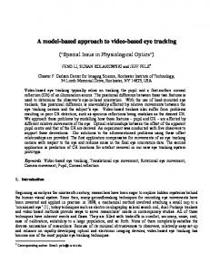
i.e., assume Tˆi ,t and X i ,t are unbiased and mutually independent estimators of Ti ,t , having variances Di ,t and Vi ,t , respectively. We refer to (27)-(28) as Model 3. Perhaps the assumption that X i ,t is an unbiased estimate of the truth is overly strong. On the other hand, it replaces assumptions of Model 1 or Model 2 about similarity of the areas included in the model. When there is evidence that Models 1 or 2 fail, Model 3 may be a viable alternative for screening. 3.2 Screening results examples We now show two examples of application of Models 1-3. Consider estimates of relative changes Ti ,t in September 2011. Models were defined separately by industries, thus the subscript for industry is omitted. Index i represents State, t stands for September 2011. The parameters of Models 1 and 2 are estimated based on combined estimates from all States within industry. Example 1. Statewide estimates of relative change, Business Services (NAICS Sectors 54, 55, 56). a.

b.

Figure 1. Weighted normal plots for Business services, for (a) Model 1 and (b) Model 2 In Figure 1, we show weighted normal plots for Model 1 and Model 2 based standardized residuals, along with the 95% pointwise critical regions (based on Dempster and Ryan 1985). The dashed horizontal lines are drawn at -2.5 and 2.5 levels chosen as cutoffs for “suspicious” values of the standardized residuals. These are the thresholds h that we alluded to in Section 1. According to the plots, both models provide reasonable fit. According to Model 1, in one State (Michigan, i  26 ), the estimate may need further

investigation (here, r26,t  3.5 .) Note that according to the Model 2 results, there is no values outside (-2.5,2.5) interval. This happened because the value of variance V26,t for

X 26,t in Michigan is relatively large, thus reducing our “trust” in

X 26,t (here,

r26,t  1.83 .)

Figure 2. Weighted normal plots for Business services, Model 3 The Model 3 residuals are somewhat above the reference line (see Figure 2). This confirms the fact that having the adjustment factor  greater than 1 would be an improvement. Example 2. Statewide estimates of relative change in Information (NAICS Sector 51). a.

b.

Figure 3. Weighted normal plots for Information, for (a) Model 1 and (b) Model 2 This is an example of model failure (see Figure 3). Apparently, forecasted values X i ,t cannot be uniformly “adjusted” using a single factor  across all States in this industry.

The Model 3 plot (see Figure 4) also shows that a number of States does not fit the assumption that   1 . There is the tendency in a group of States to be higher than corresponding values of X i ,t , rather confirming that the forecasts based on history are not good estimates of the current employment in these States and, in a sense, supporting validity of the sample based estimates.

Figure 4. Weighted normal plots for Business services, Model 3

4. Summary In this paper, we proposed a method of screening direct sample based estimates before their release for publication. The method is easy to use and it may become a convenient tool for the analysts. It is important to keep in mind that the method (as, in truth, would be any screening procedure) is based on assumptions. As with any model, the assumptions may fail. In fact, an important advantage of the proposed approach is that it makes explicit assumptions. Model checking, for example, using the normal plots, is essential. The plots also provide analysts with additional graphical tool to aid in their decisions.

References Bureau of Labor Statistics (2004), Chapter 2, “Employment, hours, and earnings from the Establishment survey,” BLS Handbook of Methods. Washington, DC: U.S. Department of Labor. http://www.bls.gov/opub/hom/pdf/homch2.pdf Dempster, A. P. and Ryan, L. M. (1985). Weighted normal plots. Journal of the American Statistical Association, 80 845-850. De Waal, T. (2009). Statistical Data Editing, Handbook of Statistics, Sample Surveys: Design, Methods and Applications, Eds. D. Pfeffermann and C.R. Rao, Amsterdam:Elsevier BV. Vol. 29A, Ch. 9 Fay, R.E. and Herriot, (1979). Estimates of Income for Small Places: an Application of James-Stein Procedure to Census Data, Journal of American Statistical Association, 74, 269-277

Hampel, F.R., Ronchetti, E.M., Rousseeuw, P.J. and Stahel, W.A. (1986). Robust Statistics: the Approach Based on Influence Functions. New-York, John Wiley & Sns, Inc. Huber, P. J. (1964). Robust estimation of a location parameter, Ann. Math. Statist. 35: 73–101.