Model--based Motion Estimation of Elastic Surfaces for Minimally ...

Model-based Motion Estimation of Elastic Surfaces for Minimally Invasive Cardiac Surgery Thomas Bader, Alexander Wiedemann, Kathrin Roberts, and Uwe D. Hanebeck Abstract— In order to assist surgeons during surgery on moving organs, e.g. minimally invasive beating heart bypass surgery, a master-slave system which synchronizes surgical instruments with the organ’s motion is desired. This synchronization requires reliable estimation of the organ’s motion. In this paper, we present a new approach to motion estimation based on a state motion model for a partition of the heart’s surface. Its motion behavior is described by a partial differential equation whose input function is assumed to be periodic. An estimator is used on one hand to predict future model states based on reconstruction of the input function and on the other hand to incorporate noisy spatially discrete measurements in order to improve state estimation. The model-based motion estimation is evaluated using a simple heart simulator. Measurements are obtained by reconstructing 3D position of markers on a pulsating membrane by means of a stereo camera system.

image processing

View on the stagnant heart

View on the beating heart estimation of heart motion

head mounted display

camera system

manipulator

haptical interface

Fig. 1.

manipulator control

Overview of the system architecture.

I. I NTRODUCTION During open or minimally invasive beating heart bypass surgery, the area of interest is mechanically stabilized. However, significant residual motion in this area remains [1] and the surgeon has to follow this motion, which demands high concentration. In order to assist surgeons while operating on the beating heart, an active system, e.g. a robot that follows the heart’s motion based on motion estimation, is desired. The surgeon controls the robotic system while referring to a still image of the intervention area on a monitor, thus gaining the impression of operating on the motionless organ. An overview of this concept, first introduced in [2], is shown in Fig. 1. A promising approach to generate a still image of a moving surface using real-time binocular eye tracking is proposed in [3]. Master-slave robotic systems like ZEUS and da Vinci are already used, but do not offer active autonomous motion synchronization with the beating heart. For this synchronization a method for exact motion prediction , based on measurements of heart motion, for each point of interest (POI) on the organ’s surface is necessary. In earlier studies, several motion compensation algorithms and measurement methods were discussed. In order to predict the heart’s motion at a POI in one direction, a displacement model with weighted Fourier series is used [4]. The POIdeflection is measured by a fibre-optic laser sensor. In [2], 2D-motion of a POI is estimated with an autoregressive model based on 2D prior position measurements by a single camera. An approach for 3D-recovery of soft tissue deformation is proposed in [5]. Image rectification combined T. Bader, A. Wiedemann, K. Roberts, and U. D. Hanebeck are with the Intelligent Sensor-Actuator-Systems Laboratory, Institute of Computer Science and Engineering, Universit¨at Karlsruhe (TH), Germany. {thomas.bader|wiedemann}@ira.uka.de, {kathrin.roberts|uwe.hanebeck}@ieee.org

with constrained disparity registration is used to gain 3D information about the surface directly from a stereo image pair. This approach offers no possibility for estimating the position of occluded surface parts, which can be caused for example by surgical instruments. In [6], natural landmarks on the heart surface are tracked by a single camera. They propose a method for predicting motion of surface points based on their x- and y-trajectories, respiration pressure signal, and ECG signal observed in the past. Those features are tracked robustly even with short-time occlusions. A predictive-control approach on filtering the heart motion is presented in [7] and [8]. In [7], a 6 DOF robot is set up, which is synchronized with an oscillating target using visual servoing techniques and a modified generalized predictive controller to learn and predict the organ’s motion. The modelbased predictive controller described in [8] is based on a motion model containing sonomicrometry measurements of the POI-trajectory out of the past heart beat cycle. Additionally, in [8] the prediction is improved by detecting changes of heart beat period in the ECG signal. The above mentioned methods do not describe the connections between the measurable or occluded POI and other measurable points by means of a surface model. Such a model could, however, include the distributed motion and facilitate the POI reconstruction. In this paper, we present a fundamental model-based approach for reconstructing the position of any arbitrary POI and for predicting the heart’s surface motion in the intervention area. The key idea of our approach is that a partition of the heart surface is represented by a pulsating membrane model. The motion behavior of the membrane is described using a partial differential equation (PDE) whose input function is assumed to be periodic. An estimator is used for predicting future model states based on reconstruction

of the input function (similar to [4]) and to improve state estimation by incorporating noisy spatially discrete measurements from a real system. The advantage of this approach is that state estimation can be used to reconstruct the whole surface of the partition based on discrete measurements. The model-based motion estimator is evaluated using an experimental setup, where markers attached to a pulsating membrane are tracked by a stereo camera system (see Fig. 2). Model-based prediction is used to identify markers in consecutive image frames. The remainder of this paper is organized as follows. Section II gives a general problem formulation for motion estimation of elastic surfaces. In Section III model equations are derived and the estimator used is presented. Section IV describes the experimental setup and software of the testbed. In Section V results of model-based motion estimation for the pulsating membrane are shown. II. P ROBLEM F ORMULATION As already mentioned in the previous section, modelbased surface reconstruction and estimation opens up new possibilities for motion compensation in minimally invasive surgery, particularly for beating heart bypass surgery. In this section, the problem of motion estimation of an organ’s surface is formulated in a general manner. Then, by making certain assumptions, these problems are restricted to the special case of a circular partition of an organ’s surface with linear elastic material behavior. In general, the problem of model-based motion estimation of an organ’s surface can be separated into two subproblems. The first one consists of mathematically describing the motion behavior of the surface as a distributed phenomenon. The surface motion model is usually formulated as a distributed parameter system, which has to consider specific material properties as well as muscle contraction or external forces that affect and deform the surface. In order to estimate the system’s state, it has to be converted into a lumped parameter system. The behavior of a discrete-time lumped parameter system can be described by the system equation, which can either be linear, such as xk+1 = Ak xk + Bk (uk + wk )

Pulsating membrane and tracking system.

means of the stochastic system equation as well as a filter step to improve estimation of the system state with noisy measurement. The choice of an estimator initially depends on whether system and measurement equations are linear or nonlinear. While a Kalman Filter [9] can be used for the linear case, nonlinear filters such as Extended Kalman Filter or Progressive Bayes [10] can be used for the nonlinear case. Regarding the problem of reconstructing the surface and estimating the motion of a partition of a beating heart, some assumptions can be made. The shape of the partition and boundary conditions are determined by the stabilizer, which is used for stabilizing the heart. In this paper, the partition is assumed to be of circular shape with fixed boundary conditions. The elasticity of the organ’s material is assumed to be linear and the organ moves periodically. With these assumptions the motion model can be designed, which finally leads to the system equation. For obtaining measurements, a binocular system is used, which enables 3D-tracking of markers attached to the surface as shown in Fig. 2. In order to track particular markers, they need to be uniquely identified in consecutive image frames. The model-based predictions for marker positions can be used in order to recover the corresponding marker in the next image frame and to restrict the search area.

(1)

or nonlinear. In (1), xk and xk+1 are chronologically consecutive system states related to each other by Ak . Matrix Bk relates the control input uk , which can either be muscle contraction or external forces, to state xk+1 and wk describes process noise. The second subproblem is concerned with estimation of the real system state based on system description and measurements. For this purpose, the system state xk has to be related to measurements y k . This measurement equation can either be linear, such as y k = Hk xk + v k

Fig. 2.

(2)

or nonlinear. In (2), v k is the measurement uncertainty. Furthermore, an appropriate estimator has to be chosen, which contains a predictor for estimation of future states by

III. A M ODEL FOR S URFACE E STIMATION OF A C IRCULAR M EMBRANE In order to describe and predict the behavior of a circular partition of an organ’s surface, the state system model is derived by means of a membrane model (III-A), the measurement equation is derived and the state estimator has to be chosen (III-B). In [11], approaches for reconstruction and prediction of stochastic distributed linear system are proposed. As the motion behavior of the membrane is described by a linear PDE, an approach from [11] is basically used. In [11], the control input uk is known and predefined. The novelty in this paper in contrast to [11] is that the input function is represented by a Fourier series and its parameters are adapted during data processing to reconstruct a real periodic input function.

A. System Equation In this section, the linear PDE describing the motion behavior of the system is first derived. Then it is converted into a system equation as in (1) using the two-step process similar as described in [11]. The starting point for deriving a mathematical description for motion behavior of a circular membrane with isotropic elastic material are the Lam´e differential equations. They are denoted with j = 1, 2, 3 as follows for the three-dimensional case (λ + μ)(

3  ∂ 2 ui ∂ 2 uj ) + μ∇2 uj + (fj − ρ 2 ) = 0 . (3) ∂xj ∂xi ∂t i=1

λ and μ are the so-called Lam´e moduli describing the elastic properties of the medium. ui = ui (x1 , x2 , x3 , t) describes the deflection in xi direction at surface point (x1 , x2 , x3 ) and time t. fi is an external force affecting the membrane in xi direction and ∇2 is the Laplace-operator. As a simplifying constraint, the deflection is assumed to only occur in direction x3 , which is perpendicular to the (x1 , x2 )-plane of the membrane as shown in Fig. 2. This leads to ∂2u )=0 , (4) ∂t2 where u := u3 and f := f3 . In order to incorporate the damping, which occurs in the system, a velocity dependent damping term du˙ is added to (4). For easier handling, coordinates are converted from cartesian to polar, whereas r and ϕ denote radius and angle, respectively. This results in 1 ∂u 1 ∂ 2 u ∂2u ∂u ∂2u μ( 2 + 2 + = −f , (5) ) − ρ −d ∂r r ∂r r ∂ϕ2 ∂t2 ∂t μ∇2 u + (f − ρ

with u = u(r, ϕ, t). Boundary conditions, describing the circular shape of the membrane are given by u(a, ϕ, t) = 0 ,

∞ 

ui (r, ϕ, t) ≈

i=1

N EF 

N  2 M   m=1 n=0 i=1

The number of eigenfunctions is NEF = 2M (N + 1). In contrast to [11] in this paper the approximated solution (7) is not transformed into a normalized form and the excitation function f of the inhomogeneous PDE is described in a different way. f is decomposed into spatially and timedependent parts as follows f (r, ϕ, t) ≈

N TE 

Xi (r, ϕ)pi (t) .

(9)

i=1

The time-dependent parts pi of (9) are approximated by the Fourier series pi (t) = ci +

N TP 

aij cos(jωt) + bij sin(jωt) .

(10)

j=1

The spatially dependent parts Xi are assumed to be known. In this paper, pi is assumed to be periodical with constant frequency ω. Therefore ci , aij and bij are the only parameters that need to be determined in (10). Inserting formulas (7) and (9) into the inhomogeneous PDE (5) according to [11] results in μ −ρ

N EF 

1 1 (∂rr + ∂r + 2 ∂ϕϕ )ψi (r, ϕ)αi (t) r r i=1

N EF 

ψi (r, ϕ)¨ αi (t) − d

i=1

=−

N EF 

i=1 N TE 

ψi (r, ϕ)α˙ i (t)

(11)

Xi (r, ϕ)pi (t),

i=1

ψi (r, ϕ)αi (t) .

(7)

i=1

For a circular membrane with boundary conditions (6), this leads to u(r, ϕ, t) =

Umn1 = cos(nϕ)Jn ( ar cmn ) and Umn2 = sin(nϕ)Jn ( ar cmn ) .

(6)

where a denotes the radius of the membrane. In order to convert (5) to an equation of the form (1), the homogeneous part of the linear PDE (5) is considered first. By means of the separation method the solution uH of the homogeneous part is decomposed into a spatially dependent part ψ and a time-dependent part α. Then the particular solution is calculated and adapted to the boundary conditions. In general, this results in several solutions. The solutions are characterized by eigenvalues. Due to the linearity of the PDE, the superposition of all solutions is also a solution of the homogeneous part of equation (5). Finally, the solution is approximated by a finite number NEF of eigenfunctions, which results in u(r, ϕ, t) =

where cmn is the m-th zero point of a Bessel function Jn (t) of first kind and order n. In (8), c = μρ , Umn1 and Umn2 are given by

Amni Umni (r, ϕ) cos(

ccmn t ), (8) a

which has to be satisfied at any arbitrary point. In order to spatially discretize (11), a finite number NCP of collocation points is chosen, where (11) has to be fulfilled. After inserting the collocation points into (11), the equations are summarized to the form μ ψ μ α(t) − d ψ d α(t) ˙ − ρ ψ ρ α(t) ¨ = −Xp(t)

(12)

where ψ d , ψ ρ ∈ IRNCP ×NEF contain spatially dependent eigenfunctions, ψ μ ∈ IRNCP ×NEF contains spatially derivations of the eigenfunctions and X ∈ IRNCP ×NT E contains the predetermined spatially dependent functions Xi of (9). ¨ in (12) are known at time tm , setpoints If α, α˙ and α pSi (tm ) for each pi (tm ) from (10) can be calculated by inverting X in (12). In order to reconstruct ci , aij and bij adequately, the condition ci +

N TP 

!

aij cos(jωtm ) + bij sin(jωtm ) = pSi (tm )

(13)

j=1

has to be satisfied. This equation is under-determined and has an infinite number of solutions. In order to reconstruct the

desired parameters anyway, not only one setpoint is used, but also setpoints for past points in time are considered. Thus, a linear system of equations is obtained from (13) for each setpoint, which can be used to calculate ci , aij and bij . The reconstruction process of the excitation function (9) is included in the filter step of the estimator as discussed in (III-B). The lumped parameter system (12) of order two is reduced with the corresponding matrices E, A, B to the form ˙ = Aβ(t) + B(u(t) + w(t)), Eβ(t)

(14)

T ˙ is defined as the system state. The where β = (α(t), α(t)) term w(t) is an additive noise term with covariance Q and describe the zero mean process noise. In order to obtain an equation as in (1), equation (14) has to be transformed. If E is regular, it can just be inverted. If (14) is over-determined, i.e., NEF < NCP , rank(E) = NEF and rank(Q) = NCP , the least squares method can be used to calculate the pseudoinverse of E. Otherwise, if rank(E) < NEF , (14) is a descriptor system. Literature regarding solutions for that problem can be found in [11]. After the time-discretization of (14), a system equation as in (1) is finally obtained.

B. Measurement- and Kalman Filter Equations In the previous section, the linear stochastic system equation, describing the motion behavior of a circular oscillating membrane, was derived. Because the state β k of the system equation is estimated, one has to improve the estimation of the state by means of measurements of the real system. In this section, the measurement equation is defined and the state estimator used to predict and reconstruct the surface deflection of the membrane is described. If measurements y k at time tk directly refer to membrane deflection u and deflection velocity u˙ in x3 -direction (see Fig. 2) at certain measurement points, a linear mapping of the derived state β k onto measurements y k by means of relation (7) can be derived. For the measurements y k , a zero mean noise value v k with covariance Rk is assumed, so that a linear measurement equation as in (2) is obtained. Thereby Hk contains the spatially dependent eigenfunctions ψ for any measurement points as described in [11]. Because the system and measurement equations are linear, and additive zero-mean process noise and measurement noise is assumed, the well-known Kalman Filter is used for the estimation of the state β k . The estimator consists of two main steps: the filter step and the prediction step. The equations of the filter step are equal to those discussed in [11]. The characteristics of the estimated state are described by its ˆ and its covariance matrix Ck . After expectation value β k improving the estimation of the state β k with measurements y k , the excitation function f as described in Section III˙ α ¨ of (12) A is reconstructed. First of all the values α, α, are estimated and the matrix X is inverted to obtain the setpoints. After this the coefficients of the Fourier series (10) are determined. The obtained Fourier series for p is used to determine the excitation function for the next prediction step. In the prediction step, the state estimation β k is updated to

Fig. 3.

Testbed and enlarged surface section.

β k+1 by means of the state equation obtained by (14). The excitation function is calculated via the reconstructed p of the last filter step. Also the covariance matrix Ck is updated (see [11]). Now the used estimator is described, the only thing that is still missing is the reconstruction of the surface deflection at every point. With the estimation of state β k the deflection at each point can be reconstructed with the approximated ˆ k . The solution function (7) as u(r, ϕ, tk ) ≈ ψ(r, ϕ)T α quality of the model-based estimator derived above will be evaluated in the following section. IV. M ODEL E VALUATION For evaluating the stochastic surface model, a pulsating membrane as shown in Fig. 3 was used. Apart from that, the model-based motion estimator introduced in Section III was implemented and image processing software, to gather measurements, was written. In this section the testbed and implemented software systems are described. A. Experimental Setup In this section, the experimental setup for evaluating the model-based motion estimator derived in III is described. A moving circular partition of a heart’s surface is simulated by a thin elastic membrane bounded by a circular aperture in a metal plate as shown in Fig. 3. The membrane oscillates with a constant frequency, which can be set arbitrarily between about 0.5 and 2.4 Hz. In order to acquire measurements of particular surface points, circular markers are attached to the membrane and are tracked using a stereo camera system and corresponding image processing algorithms. B. Image Processing In order to obtain measurements of the deflection of the membrane at discrete surface points, markers stuck to the membrane’s surface (see Fig. 3) are tracked. In this section, initialization as well as functionality of the image processing system using Intel’s OpenCV library is described. During initialization, the intrinsic and extrinsic camera parameters needed for 3D depth recovery are computed. The fundamental matrix for epipolar matching is calculated.

Then the diameter of the membrane, the coordinates of its center, and the plane containing the margin of the membrane are determined. From an initialization image, which is an arbitrary image from the sequence, measuring points are chosen. Later on, only the distances between these surface points to their projections into the membrane plane serve as measurements. To speed up feature extraction and stereo matching, the size of the landmarks as well as the search areas in each camera image can be specified. Image processing is done in three major steps: Extraction of marker positions, stereo-matching, and reconstruction of 3D coordinates. Features are extracted from both, the left and right camera images independently using the Canny edge detection algorithm and ellipsoid fitting methods supplied by OpenCV. The matching of corresponding features is realized by epipolar matching combined with a relative position constraint to reduce search space along the epipolar line. For each pair of matched features, 3D coordinates are computed. C. Implementation of the Model-based Estimator and Interaction with Image Processing Fig. 4 illustrates the interaction between the model-based estimator and the image processing components. The modelbased estimator was implemented in MATLAB. The MATLAB methods are called from the C++ part using the MATLAB COM-interface. For setting model parameters, the function init(M, N, NCP , NT E , NT P , μ, d, ρ, ω, rm , ϕm ) has to be executed. M , N , NCP , NT E , NT P , μ, d, ρ and ω are declared in Section III. rm and ϕm contain radii and angles of the surface points for which the deflections should later be predicted. Since the real deflection of the membrane is only known at marker positions, only estimations at those points can be evaluated. Therefore, rm and ϕm in this case exclusively contain marker positions. From these marker positions the NCP collocation points are selected randomly. In this evaluation, the measurement points are equated to the collocation points. Besides the initialization routine, the implementation provides two methods: update(u, mask, tm ) and estimate(tk ). update is called to provide new measurements. u contains the measured distances between the collocation points and the membrane plane. mask is used to indicate whether measurements at certain collocation points are available at time tm . Therefore, the model state can be updated even if measurements could not be obtained at all collocation points, for example due to occlusion. During update the filter step of the estimator (see Section III-B) is executed and improves the estimation of β. By calling estimate, the ˆ prediction step is executed. With the received estimation β, the deflections for any arbitrary point can now be computed. The function estimate returns the predicted deflections for the marker positions used by the image processing software to track the markers over subsequent image frames. V. E XPERIMENTS In this section, first experimental results regarding modelbased surface estimation of the circular membrane are discus-

Fig. 4.

Interaction of system components.

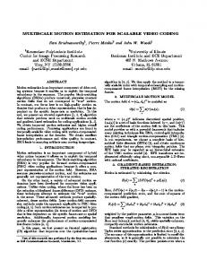
sed. Afterwards, the influence of tracking the markers using the model-based predictions (see Section IV-C) on robustness of estimations is described. Fig. ?? shows measured and predicted deflection of a noncollocation point on the circular membrane. Image series for that experiment were taken with a frame rate of 72 fps while the membrane was oscillating at ω = 0.653 Hz. Resolution of camera images is 320x320 pixels, which corresponds approximately to a ratio of 0.45 mm/pixel. The membrane used has radius a of 6 cm and is shown in Fig. 3. Attached markers have a diameter of 5 mm. The number of collocation points was set to 30 and 21 eigenfunctions were used to model the surface. Results in Fig. ?? show, that deflection of the oscillating surface is predicted quite accurately at a non-collocation point. The comparison of predicted and actual deflection at other surface points of the membrane shows similar results. Prediction error is 1.39 mm in average with a maximum value of 6.8 mm. The maximum occurs only during the fast up- and downward movements of the membrane. This relatively large error originates from a phase shift of the reconstructed excitation function compared to the real excitation. This delay of approximately 0.03 s is probably caused by unexact material parameters, which were empirically adapted to μ = 9.5, d = 0.1 and ρ = 0.08. The error of time shifted predicted deflections for a single point is shown in Fig. 6. Generally, predictions for markers close to borders of the membrane are slightly worse, because boundary condition (6) is not fulfilled exactly by the membrane shown in Fig. 3. For the considered data only an average of 15 out of 30 measurement points was available. This shows the robustness of predictions towards the absence of measurements at single collocation points. Another issue is the robustness of the tracking procedure described in IV-C. Since model-based prediction with accurate material parameters is used to find corresponding markers in consecutive image frames, those markers, which were lost for example due to occlusions or reflections, can be retrieved again. On the other hand, if the material parameters are inaccurate the prediction is also inaccurate and the markers may be tracked wrongly. This inaccuracy leads to predictions

predicted deflection / cm

0.5

1

0.5

0

0

−0.5

measured deflection / cm

measured deflection predicted deflection

1

−0.5

0

1

2

3

4

5

6

7

8

9

time / s

Fig. 5.

Results at non-measurement point p = (0.63, 0.38).

VII. ACKNOWLEDGEMENTS This work was partly supported by the German Research Foundation (DFG) within the Research Training Group GRK 1126 “Development of New Computer-based Methods for the Future Working Environment in Visceral Surgery”. The theoretical basis of this work has been established in the diploma thesis “A Modal Approach for the Prediction of the Motion of Elastic Bodies” by Rainer Misch.

4.5

4

prediction error / mm

3.5

3

2.5

R EFERENCES

2

1.5

1

0.5

0

1

2

3

4

5

6

7

8

9

time / s

Fig. 6.

surface our approach has to be extended. The membrane model has to be formulated for a deflection in all three dimensions. The 3D model-based estimator has to adapt the parameters of the model to each patient’s heart individually. Furthermore, it has to be extended to be robust against irregularities in the excitation function and changing excitation frequencies. If it turns out that the linear model is not sufficient for predicting real heart motion, it has to be extended to the nonlinear case. In this context and to consider more complex boundary conditions, the approach proposed in [12] might be more suitable. In further research work, real-time capability of the system has to be evaluated and assured.

Error for time shifted prediction at point p = (0.63, 0.38).

even worse and to instability in ensuing time steps. VI. C ONCLUSION In this paper, a fundamentally new model-based approach for estimating the motion of a circular partition of an organ surface is proposed. The periodically moving organ surface is represented by a pulsating membrane model which material behavior is assumed to be linear. The deflection behavior of the membrane is described by a linear inhomogeneous PDE. By means of modal analysis and collocation method, the PDE is converted to a lumped parameter system. The unknown periodical input function is represented by a Fourier series. A linear measurement equation, which maps the model state to 3D position measurements of the membrane surface is defined. The derived equations are used together with the Kalman Filter to predict the model state based on the reconstructed input function and in order to reconstruct z-deflection of the surface in any arbitrary point. The state prediction is also used to identify markers attached to the membrane over consecutive image frames. Evaluation using a pulsating membrane instead of a real heart surface showed promising prediction and reconstruction results. In order to use the model-based estimator to synchronize manipulators of a master-slave system with the moving heart

[1] P. Cattin, H. Dave, J. Gr¨unenfelder, G. Szekely, M. Turina, and G. Z¨und. Trajectory of Coronary Motion and its Significance in Robotic Motion Cancellation. In European Journal of Cardio-thoracic Surgery, volume 25, pages 786–790, 2004. [2] Y. Nakamura, K. Kishi, and H. Kawakami. Heartbeat Synchronization for Robotic Cardiac Surgery. In Proceedings of the 2001 IEEE International Conference on Robotics and Automation - ICRA 2001, pages 2014–2019, 2001. [3] G. P. Mylonas, D. Stoyanov, F. Deligianni, A. Darzi, and G.-Z. Yang. Gaze-contingent Soft Tissue Deformation Tracking for Minimally Invasive Robotic Surgery. In Medical Image Computing and ComputerAssisted Intervention - MICCAI 2005, volume 3749 of LNCS, pages 843–850. Springer, 2005. [4] A. Thakral, J. Wallace, D. Tomlin, N. Seth, and N. V. Thakor. Surgical Motion Adaptive Robotic Technology (S.M.A.R.T): Taking the Motion out of Physiological Motion. In Medical Image Computing and Computer-Assisted Intervention - MICCAI 2001, volume 2208 of LNCS, pages 317–325. Springer, 2001. [5] D. Stoyanov, A. Darzi, and G. Z. Yang. Dense 3D Depth Recovery for Soft Tissue Deformation During Robotic Assisted Laparoscopic Surgery. In Medical Image Computing and Computer-Assisted Intervention - MICCAI 2004, volume 3217 of LNCS, pages 41–48. Springer, 2004. [6] T. Ortmaier, M. Gr¨oger, D. H. Boehm, V. Falk, and G. Hirzinger. Motion Estimation in Beating Heart Surgery. In IEEE Transactions on Biomedical Engineering, volume 52, pages 1729–1740, 2005. [7] R. Ginhoux, J. Gangloff, M. de Mathelin, L. Soler, M. M. Arenas Sanchez, and J. Marescaux. Active Filtering of Physiological Motion in Robotized Surgery Using Predictive Control. In IEEE Transactions on Robotics, volume 21, pages 67–79, 2005. [8] O. Bebek and M. C. Cavusoglu. Model Based Control Algorithms for Robotic Assisted Beating Heart Surgery. In IEEE Engineering in Medicine and Biology Society - EMBC 2006, pages 823–828, 2006. [9] D. Simon. Optimal State Estimation, chapter 5. Wiley & Sons, 2006. [10] U. D. Hanebeck, K. Briechle, and A. Rauh. Progressive Bayes: A New Framework for Nonlinear State Estimation. In Proceedings of SPIE, AeroSense Symposium, volume 5099, pages 256–267, 2003. [11] K. Roberts and U. D. Hanebeck. Prediction and Reconstruction of Distributed Dynamic Phenomena Charaterized by Linear Partial Differential Equations. In Proceedings of the 8th International Conference on Information Fusion 2005, Philadelphia, 2005. [12] F. Sawo, K. Roberts, and U. D. Hanebeck. Bayesian Estimation of Distributed Phenomena Using Discretized Representations of Partial Differential Equations. In Proceedings of the 3rd International Conference on Informatics in Control, Automation and Robotics ICINCO 2006, Set´ubal, pages 16–23, 2006.