Model checking probabilistic and stochastic extensions of the Ï-calculus

Author manuscript, published in "IEEE Transactions of Software Engineering 35, 2 (2009) 209--223" IEEE TRANSACTIONS ON SOFTWARE ENGINEERING

1

Model checking probabilistic and stochastic extensions of the π -calculus

inria-00424856, version 1 - 19 Oct 2009

Gethin Norman, Catuscia Palamidessi, David Parker and Peng Wu

Abstract— We present an implementation of model checking for probabilistic and stochastic extensions of the π-calculus, a process algebra which supports modelling of concurrency and mobility. Formal verification techniques for such extensions have clear applications in several domains, including mobile ad-hoc network protocols, probabilistic security protocols and biological pathways. Despite this, no implementation of automated verification exists. Building upon the π-calculus model checker MMC, we first show an automated procedure for constructing the underlying semantic model of a probabilistic or stochastic π-calculus process. This can then be verified using existing probabilistic model checkers such as PRISM. Secondly, we demonstrate how for processes of a specific structure a more efficient, compositional approach is applicable, which uses our extension of MMC on each parallel component of the system and then translates the results into a high-level modular description for the PRISM tool. The feasibility of our techniques is demonstrated through a number of case studies from the π-calculus literature. Index Terms— Verification, Model checking, Markov processes, Stochastic processes

I. I NTRODUCTION

T

HE π-calculus [1] is a process algebra for modelling concurrency and mobility. It has been used to model, for example, communication protocols for dynamic network topologies, security protocols and biological pathways. For each class of systems, probabilistic and stochastic behaviour are often also key ingredients. Mobile ad-hoc network protocols, for example, can exhibit probabilistic behaviour through either communication failures or random back-off procedures. Similarly, randomisation is frequently applied in security protocols, e.g. for anonymity [2] or contract-signing [3]. For biological systems, the times between reactions are of a stochastic nature. Consequently, suitable variants of the π-calculus have been developed: probabilistic versions, for example [4], which extend the original calculus with discrete probabilistic choice, have been proposed as a formalism to model and reason about randomised security protocols [5], [6]; and stochastic extensions, for example [7], which augment the calculus with exponential delays, have been shown to be a suitable formalism for modelling and reasoning about complex biological pathways [8], [9]. The benefits of automatic formal verification and tool support in this context are clear: reasoning correctly about the behaviour of such models, particularly interactions between probabilistic and nondeterministic behaviour, is known to be G. Norman and D. Parker are with the Oxford University Computing ´ Laboratory, C. Palamidessi is with INRIA Saclay and Ecole Polytechnique, and P. Wu is with University College London.

non-trivial. Furthermore, the state spaces of probabilistic or stochastic models of realistic systems have a tendency to grow extremely quickly, making manual verification difficult or infeasible. In this paper, we describe an implementation of probabilistic model checking for models described in two different extensions of the π-calculus. The first, the simple probabilistic π-calculus, is an extension of the π-calculus obtained by introducing a discrete probabilistic choice operator in addition to the existing nondeterministic choice operator. The second, the stochastic π-calculus, extends the original calculus by associating rates (parameters of exponential distributions) with both silent transitions and channels. Our approach is to adapt and reuse existing tools for verification of mobile systems and of probabilistic and stochastic systems. We first developed an extension of the tool MMC [10], a logic-programming-based model checker for the πcalculus. This extension, MMCprob , can derive the semantic model for an arbitrary process in the (finite-control) probabilistic or stochastic π-calculus. The semantic model, which is given by a Markov decision process (MDP) or continuous-time Markov chain (CTMC), can then be analysed using standard tools, such as the probabilistic model checker PRISM [11]. To improve efficiency, when the process has a specific structure, we employ a compositional approach, applying MMCprob to each parallel component of a system, processing the results to produce a high-level modular description in the modelling language of PRISM and then performing probabilistic verification. This avoids a potential blow-up in the size of the intermediate MDP or CTMC representation and allows us to exploit the efficient symbolic model construction and analysis techniques in PRISM. We present experimental results to illustrate the performance of our implementation on a number of case studies. To our knowledge, this paper constitutes the first attempt to implement automated verification in this area. Related work: Various tools exist for automatic verification of the (non-probabilistic) π-calculus. The Mobility Workbench (MWB’99) [12] provides a bisimulation checker and a πµ-calculus model checker. MMC (Mobility Model Checker) [10], a more recently developed tool, also supports the π-µcalculus. The latter places particular emphasis on efficiency and is built using logic programming technology. ProVerif [13] supports verification of the applied π-calculus, a variant of the basic calculus. It is aimed primarily at analysis of cryptographic protocols and is theorem-prover based. Two alternative approaches are the PIPER system [14], which verifies π-calculus processes augmented with type signatures


2

IEEE TRANSACTIONS ON SOFTWARE ENGINEERING

based on an extraction of sound models using types and CCS processes, and [15], [16] which translate a subset of the πcalculus to the language Promela for model checking in the SPIN tool. Static analysis techniques have also been applied to the π-calculus, including abstract interpretation [17] and control flow analysis [18]. A number of existing papers have proposed probabilistic extensions of the π-calculus. The first, [4], extended the asynchronous version of the calculus, which removes the output prefix construct, meaning processes must terminate immediately after sending output. A version was then proposed in [5], considering only silent probabilistic transitions. This variant, which is essentially the same as the one used in this paper, was introduced to specify and reason about randomised security protocols. In [6], the probabilistic π-calculus was used to formalise definitions of anonymity. A stochastic extension of the π-calculus was first considered in [7] in which the action prefix construct was replaced with an action-rate prefix construct. A number of different variants have since been proposed differing in how rates are added to the prefix construct. In this paper, we follow [19] and parameterise silent (τ ) actions with rates and associate a (fixed) rate with each channel. A number of discrete-event simulators for the stochastic π-calculus are available, e.g. BioSpi [9] and SPiM [19], but to our knowledge no model checking tools. Structure: The remainder of this paper is structured as follows. Section II introduces the syntax and semantics for probabilistic and stochastic extensions of the π-calculus. Sections III and IV describe our extension of MMC for evaluating these semantics and show how the result of this extension can be processed into input for the PRISM tool. Section V presents experimental results and Section VI concludes the paper. A preliminary version of this paper (with only the discrete probabilistic case) appeared as [20]. II. T HE π- CALCULUS The π-calculus is a process algebra for modelling concurrency and mobility. Based on value-passing CCS [21], a key distinguishing feature of the calculus is that it uses a single datatype, names, for both channels and values, with the consequence that it is possible to communicate channel names between processes. In this section we present the probabilistic and stochastic extensions of the π-calculus for which we have developed automated model checking procedures. In order to facilitate model checking, we make two simple assumptions. Firstly, we restrict our attention to finite-control π-calculus processes, i.e. where recursion is not permitted within parallel composition. This is necessary to ensure that the resulting models are finitestate and is in fact also imposed by the MMC π-calculus model checker, on which our work relies. Secondly, we require that the systems to which we apply model checking are closed, intuitively meaning that they receive no inputs from their environment and send no outputs to it. This is due to the nature of the properties that are

analysed by probabilistic model checkers such as PRISM. We will discuss this issue further in Section IV-F. Preliminaries: Before describing the probabilistic variants of the π-calculus, we present some preliminary notation and definitions. Throughout the paper we will assume a countable set N of names, ranged over by x, xi , y, etc. A match is an equality test on names from N and a condition M is a finite conjunction of matches, i.e. M is of the form [x1 =y1 ] ∧ · · · ∧ [xn =yn ]. We denote by n(M ) the set of names that appear in M (ignoring any trivial equality tests of the form [x=x]). A substitution σ is a partial mapping from N to N . The simplest substitutions are of the form {y/x} which maps x to y. We let n(σ) denote the set of names that the substitution affects, i.e. n(σ) = {x | ∃y(6=x) ∈ N . σ(x)=y} ∪ {x | ∃y(6=x) ∈ N . σ(y)=x}. A substitution σ satisfies the match [x=y], denoted σ |= [x=y] if σ(x)=σ(y). Satisfaction extends to conjunctions of matches in the obvious way, e.g. σ |= [x1 =y1 ] ∧ [x2 =y2 ] if σ |= [x1 =y1 ] and σ |= [x2 =y2 ]. We will use five different action types for the two extensions of the π-calculus: τ (silent action), r(∈ R) (rate action), x(y) (input), x ¯y (output) and x ¯(y) (bound output). The bound names for an action α, denoted bn(α), are defined as follows: bn(τ ) = bn(r) = bn(¯ xy) = ∅ and bn(x(y)) = bn(¯ x(y)) = {y}. A substitution σ can also be applied to an action α, denoted ασ. The definition of this is: τ σ = τ , rσ = r, (x(y))σ = σ(x)(y) if y 6∈ n(σ), (¯ xy)σ = σ(¯ x) σ(y) and (¯ x(y))σ = σ(¯ x)(y) if y 6∈ n(σ). Note that in the case of input and bound output actions (i.e. those with bound variables), the substitution is only defined when the substitution does not change the bound names. A. The simple probabilistic π-calculus We use a probabilistic extension of the π-calculus called the simple probabilistic π-calculus or πprob , which adds a discrete probabilistic choice operator to the basic calculus. This choice operator is blind, meaning that probabilities are associated only with silent τ actions, and not input or output actions. Syntax: We will let P , Pi range over terms and α range over actions. Using, as above, x, y, yi to range over names, the syntax of the simple probabilistic π-calculus is: α ::= τ x(y) x ¯y P P ◦ P |P P ::= 0 α.P i∈I Pi i∈I pi τ.Pi νx P [x=y]P A(y1 , . . . , yn ) P where I is an index set, pi ∈ (0, 1] with i∈I pi = 1 and A is a process identifier. In the following paragraphs, we provide an informal description of the calculus. The next section presents the formal semantics. The inactive process, denoted 0, can perform no actions. The action-prefixed process α.P can perform action α and then evolve into P , where α is one of three types: x(y) inputs a name on x and stores it in y, x ¯y outputs the name y on x; and τ is the silent action representing internal communication.


NORMAN et al.: MODEL CHECKING PROBABILISTIC AND STOCHASTIC EXTENSIONS OF THE π-CALCULUS

P There are twoPtypes of choice: nondeterministic i∈I Pi and probabilistic ◦ i∈I pi τ.Pi . The former is standard in the πcalculus (and indeed CCS). The latter is the only new operator in this probabilistic extension of the π-calculus. As mentioned above, branches of the probabilistic choice P operator are always prefixed with τ actions. The process ◦ i∈I pi τ.Pi randomly selects an index i ∈ I with probability pi , performs a τ action and then evolves to process Pi . We use p1 τ.P1 ⊕ p2 τ.P2 to denote the binary form of probabilistic choice. The parallel composition P1 | P2 can either proceed asynchronously or interact through matching input/output actions. The restriction νx P localises the scope of x in process P , i.e. x can be considered a new and unique name within P . The match construction [x=y]P can evolve as process P only if the match [x=y] is satisfied, i.e. names x and y are identical. Finally, A(y1 , . . . , yn ) is a recursive call with a corresponding process definition clause of the form A(x1 , . . . , xn ) , P . An occurrence of name y in process P is bound if it is in a subexpression of P of the form x(y) (input-bound) or νy (νbound); otherwise, it is free. The sets of free and bound names of P are denoted by fn(P ) and bn(P ), respectively, and the set of all names is n(P ). Without loss of generality, we also make the assumption that bound names are all distinct from each other and from free names. This can always be achieved through alpha conversion. A process which contains no free names is said to be closed. Symbolic semantics: The operational semantics for probabilistic extensions of the π-calculus are typically expressed in terms of Markov decision processes (MDPs) or, equivalently, probabilistic automata [22], which allow both probabilistic and nondeterministic behaviour. Existing presentations of the semantics (for example [5], which describe a calculus essentially identical to πprob ) are concrete in the sense that the semantic rules directly define the MDP that corresponds to a process term. In this paper, we use a symbolic presentation of the operational semantics [23]. This approach is in fact quite common for the π-calculus and is particularly beneficial in the context of automatic tool support, as is the case here, or for development of bisimulation theories [23], [24]. The main features of the symbolic semantics, which allow one to obtain compact models, are that: • As in the late semantics of the π-calculus, the input variable of input transitions is kept as a name variable (in contrast to the early semantics, where a different transition is generated for every possible name instance) • Analogously to the match rule, in the communication rule the match between the input and the output channel is represented by a constraint (condition). In principle it is possible to define an early version of the symbolic semantics, but such a version would differ from a concrete semantics only because it would contain the free variables of the initial process (and conditions on them). Therefore, such a version would lack the “raison d’être” of the symbolic semantics: efficiently representing the effects of the run-time communications. Consider the simple process a(x) . x ¯b . 0 which inputs a name x on channel a and then uses x as a channel on which

3

to output the name b. A concrete approach to the semantics can establish that this process can accept an input on channel a, but its subsequent behaviour (which is dependent on the input x) can only be captured once it is known which other processes it will be composed with. A symbolic approach allows the semantics of a process to include variables (e.g. x) that can be used in actions (e.g. x ¯b). This allows us to adopt a compositional approach: given a parallel composition of several processes, the semantics of each of them can be computed separately in full, and then composed afterwards. The symbolic semantics of the πprob calculus is expressed in terms of probabilistic symbolic transition graphs (PSTGs). These are a simple probabilistic extension of the symbolic transition graphs of [23], previously used for the (nonprobabilistic) π-calculus [25]–[28] and for CCS [23]. Alternatively, they can be seen as a symbolic extension of Markov decision processes. Let P be a πprob process. The probabilistic symbolic transition graph (PSTG) representing the semantics of the process P is a tuple (S, sinit , Tprob ) where: • S is the set of symbolic states, each of which is a term of the simple probabilistic π-calculus; • sinit ∈ S, the initial state, is the term P ; • Tprob ⊆ S×Cond ×Act×Dist(S) is the probabilistic symbolic transition relation and is the least relation given by the rules in Fig. 1. In the above, • Cond denotes the set of all conditions (finite conjunctions of matches) over N ; • Act is a set of actions of four basic types: τ , x(y), x ¯y and x ¯(y), where x, y ∈ N ; • Dist(S) is the set of probability distributions over S. M,α

We use the notation Q −−−→ {|pi : Qi |}i for the probabilistic P symbolic transition (Q, M, α, µ) ∈ Tprob where µ(R) = Qi =R pi for any πprob term R. For simplicity we abbreviate M,α

M,α

the transition Q −−−→ {|1 : Q0 |} to Q −−−→ Q0 and omit the trivial condition true. We use multi-sets to ensure that processes with duplicate components such as Q = 12 τ.0 ⊕ 21 τ.0 τ have transitions of the form Q − → {| 12 : 0, 12 : 0|} as opposed τ 1 to Q − → { 2 : 0}. Of the four action types in Act, the first three are described in the previous section. The fourth, x ¯(y), denotes output of a bound name and is used by the rules O PEN and C LOSE to extend the scope of the bound name y. A symbolic state Q encodes a set of πprob terms. More specifically, it encodes the set of terms obtained from Q by applying substitutions to its name variables. A substitution σ is applied to a process Q, denoted Qσ, by replacing each action α in Q with ασ. Consider for example the process a(x) Q = a(x).¯ xb.0. We have that Q −−−→ Q0 where Q0 = x ¯b.0. The symbolic state Q0 represents the terms Q0 {z/x} for any name z. M,α A symbolic transition Q −−−→ {|pi : Qi |}i represents the fact, that under any substitution σ satisfying M , the process term Qσ can perform action ασ and then with probability pi evolve to process Qi σ. This is formally stated in Lemma 1

4


M,α

P RE

P ROB

α

α.P − → {|1 : P |}

bn(α) ∩ fn(Q) = ∅

M,α

C OM

P | Q −−−→ {|pi : (Pi | Q)|}i

νxM,α

P −−−−→ {|1 : P 0 |} [x=y]∧M ∧N,τ

M,y(z)

x 6∈ n(α)

C LOSE

νx P −−−−→ {|pi : νx Pi |}i

P −−−−→ {|1 : P 0 |}

P −−−→ {|1 : P 0 |} νxM,¯ y (x)

[x=y]∧M ∧N,τ

M,α

x 6= y

P −−−→ {|pi : Pi |}i

M ATCH

νx P −−−−−−→ {|1 : P 0 |}


P {y1 , . . . , yn /x1 , . . . , xn } −−−→ {|pi : Pi |}i M,α

A(y1 , . . . , yn ) −−−→ {|pi : Pi |}i

Fig. 1.

[x=y]∧M,α

{x, y} ∩ bn(α) = ∅

[x=y]P −−−−−−−→ {|pi : Pi |}i

M,α

I DE

N,¯ x(v)

Q −−−−→ {|1 : Q0 |}

P | Q −−−−−−−−−→ {|1 : νv(P 0 {v/z} | Q0 )|}

M,¯ yx

O PEN

N,¯ xv

Q −−−→ {|1 : Q0 |}

P | Q −−−−−−−−−→ {|1 : P 0 {v/z} | Q0 |}

M,α

P −−−→ {|pi : Pi |}i

R ES

Pj −−−→ {|pjk : Pjk |}jk j∈I M,α P −−→ {|pjk : Pjk |}jk i∈I Pi −

M,y(z)

M,α

P −−−→ {|pi : Pi |}i

PAR

S UM

P τ ( ◦ i pi τ.Pi ) − → {|pi : Pi |}i

A(x1 , . . . , xn ) , P

νx (true) νx [x=x] νx [x=y] νx [y=z] νx (M ∧ N )

= = = = =

true true false (x6=y) [y=z] (x6=y ∧ x6=z) (νx M ) ∧ (νx N )

The symbolic semantics for πprob , including (inset) application of operator νx to conditions

below, which relates the symbolic (PSTG) semantics of πprob , as given in Fig. 1, and the concrete (MDP) semantics, as presented e.g. in [5]. This corresponds to Lemma 2.5 in [27] which discusses symbolic semantics for the (non-probabilistic) π-calculus. In the lemma, σ M indicates that the substitution σ satisfies the condition M of the transition, and the constraint bn(α)∩(fn(P )∪n(σ)) = ∅ corresponds to the fact that bound names are not substituted in order to prevent possible conflicts between bound and free names. Lemma 1: Let P be a πprob term. M,α

(a) If P −−−→ {|pi : Pi |}i , then for any substitution σ such ασ that σ M with bn(α) ∩ (fn(P ) ∪ n(σ)) = ∅, P σ −−→ {|pi : Pi σ|}i . α (b) If P σ − → {|pi : Pi0 |}i and bn(α) ∩ (fn(P ) ∪ n(σ)) = ∅, M,β then P −−−→ {|pi : Pi |}i where σ |= M and (β.Pi )σ = α.Pi0 . Proof: Since the symbolic and concrete semantics of πprob share the same types of actions as the (standard) π-calculus, the proof follows the one for Lemma 2.5 in [27] which is straightforward by transition induction. B. The stochastic π-calculus We now describe a stochastic extension of the π-calculus denoted πstoc , the underlying semantics of which is expressed in terms of continuous-time Markov chains (CTMCs). Each transition will thus be labelled with a rate, representing the parameter of an exponential distribution characterising the delay until the associated transition is enabled. More precisely, for rate r, the probability that the transition is enabled within t time-units is given by 1−e−r·t . As in [19], stochastic behaviour is introduced at the syntactic level by associating a

rate with each channel x, denoted rate(x), and by annotating silent τ actions with the rate r at which they occur, i.e. τr . Syntax: Using P , Pi to range over terms and α to range over actions, the syntax of the stochastic π-calculus is: α ::= τr x(y) x ¯y P P |P P ::= 0 α.P i∈I Pi νx P [x=y]P A(y1 , . . . , yn ) where r ∈ R>0 , I is an index set and A is a process identifier. As in the probabilistic case, the terms 0, P1 | P2 , νx P , [x=y]P and A(y1 , . . . , yn ) denote inactivity, parallel composition, restriction, match and recursive call. The prefix process τP r .P can (internally) evolve to P with rate r. The choice i∈I Pi represents a race condition between the transitions of each Pi : the first of these transitions to become enabled is the one that is taken. Race conditions also arise from parallel composition (P1 | P2 ) between processes. In this case, when two processes synchronise on matching input/output actions on a channel x, the rate of this transition is rate(x). Symbolic semantics: The operational semantics for the stochastic π-calculus is in terms of CTMCs. Usually (as in e.g. [19], on which our syntax is based), a concrete semantics is presented which maps each process term directly to the CTMC it represents. However, as for the probabilistic case (see the discussion in the previous section), in order to adopt a compositional approach we employ a symbolic semantics based on an extension of symbolic transition graphs [23]. Let P be a πstoc process. The stochastic symbolic transition graph (SSTG) representing the semantics for the process P is a tuple (S, sinit , Tstoc ) where: • S is the set of symbolic states, each of which is a term of the stochastic π-calculus;


5

M,α

P REτ

P RE IN

r

τr .P − →P

x(y)

P RE OUT

x ¯y

x ¯y.P −→ P

x(y).P −−−→ P

M,y(z)

M,α

P −−−→ P 0

PAR

bn(α) ∩ fn(Q) = ∅

M,α

C OM

P | Q −−−→ P | Q

P −−−−→ P 0

νxM,α

[x=y]∧M ∧N,rate(x)

M,y(z)

x 6∈ n(α)

P −−−−→ P 0

C LOSE

νx P −−−−→ P 0 P −−−→ P 0 νxM,¯ y (x)

[x=y]∧M ∧N,rate(x)

M,α

x 6= y


[x=y]∧M,α

{x, y} ∩ bn(α) = ∅

[x=y]P −−−−−−−→ P 0

M,α

P {y1 , . . . , yn /x1 , . . . , xn } −−−→ P M,α

A(y1 , . . . , yn ) −−−→ P 0

Fig. 2.

P −−−→ P 0

M ATCH

νx P −−−−−−→ P 0

I DE

N,¯ x(v)

Q −−−−→ Q0

P | Q −−−−−−−−−−−−−→ νv(P 0 {v/z} | Q0 )

M,¯ yx

O PEN

N,¯ xv

Q −−−→ Q0

P | Q −−−−−−−−−−−−−→ P 0 {v/z} | Q0

M,α

P −−−→ P 0

R ES

Pj −−−→ Pj0 M,α 0 j ∈ I P P −−−→ Pj i i∈I

S UM

νx (true) νx [x=x] νx [x=y] νx [y=z] νx (M ∧ N )

0

A(x1 , . . . , xn ) , P

= = = = =

true true false (x6=y) [y=z] (x6=y ∧ x6=z) (νx M ) ∧ (νx N )

The symbolic semantics for πstoc , including (inset) application of operator νx to conditions

sinit ∈ S, the initial state, is the term P ; • Tstoc ⊆ S×Cond ×Act×S is the stochastic symbolic transition multi-relation and is the least multi-relation given by the rules in Fig. 2. In the above, • Cond denotes the set of all conditions (finite conjunctions of matches) over N ; • Act is a set of actions of four basic types: r, x(y), x ¯y and x ¯(y), where r ∈ R>0 and x, y ∈ N . The fact that we have used a multi-relation is standard for stochastic process algebras [29] and ensures that multiple transitions are generated for expressions with identical components, such as τr .P + τr .P . This requirement is because the choice operator is interpreted as a race condition: the first transition to become enabled is the one that is taken. More precisely, since the minimum of two exponential distributions with rates r1 and r2 is an exponential distribution whose rate is the sum r1 +r2 , the behaviour of the process τr .P + τr .P should be the same as that of τ2r .P . This is captured in the semantics by the inclusion of two separate transitions labelled r in the multi-relation Tstoc . Analogously to the case for PSTGs, discussed in the preM,α vious section, a stochastic symbolic transition Q −−−→ Q0 of an SSTG represents the fact that, under any substitution σ satisfying M , the process term Qσ can perform action ασ and then evolve to process Q0 σ. This is formally stated in Lemma 2 below, which relates the symbolic (SSTG) semantics of πstoc , as given in Fig. 2, and the concrete (CTMC) semantics, as found in [19]. Again, this corresponds to Lemma 2.5 in [27] for the standard (non-probabilistic) π-calculus. •

Lemma 2: Let P be a πstoc term. M,α (a) If P −−−→ P 0 , then for any substitution σ such that ασ σ M with bn(α) ∩ (fn(P ) ∪ n(σ)) = ∅, P σ −−→ P 0 σ.

α

(b) If P σ − → Q0 and bn(α) ∩ (fn(P ) ∪ n(σ)) = ∅, then M,β P −−−→ Q where σ |= M and (β.Q)σ = α.Q0 . Proof: Straightforward by transition induction. The details are almost identical in structure to Lemma 2.5 of [27] except that the action τ in the π-calculus is replaced by numerical rates r in πstoc , which do not influence names. Strictly speaking, the concrete semantics used above do not correspond precisely to the usual definition of a CTMC, since transitions can be associated with either rates (for τ actions) or inputs/output actions (which have yet to be matched). Furthermore, multiple transitions can occur between the same pair of states (due to the use of a multi-relation in the definition of an SSTG). In the semantics of a closed πstoc process, however, only rate-labelled transitions remain and multiple transitions between states are simply summed. III. G ENERATING PSTG S AND SSTG S USING MMC In this section we describe the automatic generation of the symbolic transition graph for an arbitrary process expressed in either the simple probabilistic π-calculus or stochastic πcalculus. This is achieved with an extension of the (nonprobabilistic) π-calculus model checker MMC [10], which from this point on we refer to as MMCprob . In the next section we will build upon this, presenting a more efficient, compositional scheme for processes of a specific structure. MMCprob is based on only a subset of MMC’s functionality: essentially the capability to construct the full set of reachable states of a π-calculus process. The restrictions placed on the syntax of the calculus by MMC are the same as we impose in Section II. MMC works by (and derives its efficiency from) exploiting the similarity between the way in which resolution-based


6


% PRE: trans(pref(act, P), [pstep(1, act, P)], true). % PROB: trans(prob_choice(ProbBranches), PSteps, true) :- prob_branch(ProbBranches, PSteps). prob_branch([], []). prob_branch([pref(tau(FirstProb), P)|Others],PSteps) :prob_branch(Others, OtherPSteps), append([pstep(FirstProb, tau, P)], OtherPSteps, PSteps). % SUM: trans(choice(Branches), PSteps, M) :length(Branches, Size), upto(Size, I), ith(I, Branches, Branch), trans(Branch, PSteps, M). % PAR: trans(par(P, Q), PSteps, M) :trans(P, PPSteps, M), set_par_psteps(PPSteps, Q, PSteps, 0). trans(par(P, Q), PSteps, M) :trans(Q, QPSteps, M), set_par_psteps(QPSteps, P, PSteps, 1). set_par_psteps([], _, [], _). set_par_psteps([pstep(Prob, A, P)|Others], Q, PSteps, Which) :set_par_psteps(Others, Q, OtherPSteps, Which), (Which == 0 -> append([pstep(Prob, A, par(P, Q)], OtherPSteps, PSteps)). ; append([pstep(Prob, A, par(Q, P)], OtherPSteps, PSteps))). % RES: trans(nu(Y, P), PSteps, M) :trans(P, PPSteps, M), not_in_any(Y, PPSteps), not_in_constraint(Y, M), set_nu_psteps(PPSteps, Y, PSteps). set_nu_psteps([], _, []). set_nu_psteps([pstep(Prob, A, P1)|Others], Y, PSteps) :set_nu_psteps(Others, Y, OtherPSteps), append([pstep(Prob, A, nu(Y, P1))], OtherPSteps, PSteps). % COM: trans(par(P, Q), [pstep(1, tau, par(P1, Q1))], (M, N, L)) :trans(P, [pstep(1, A, P1)], M), trans(Q, [pstep(1, B, Q1)], N), complement(A, B, L). % OPEN: trans(nu(Y, P), [pstep(1, outbound(X, Z), P1)], M) :trans(P, [pstep(1, out(X, Z), P1)], N, V), Y == Z, Y \== X, not_in_constraint(Y, M). % CLOSE: trans(par(P, Q), [pstep(1, tau, nu(W, par(P1, Q1)))], (M, N, L)) :trans(P, [pstep(1, A, P1)], M), trans(Q, [pstep(1, B, Q1)], N), comp_bound(A, B, W, L). % MATCH: trans(match((X=Y), P), PSteps, M) :- X == Y, trans(P, PSteps, M). trans(match((X=Y), P), PSteps, (X=Y, M)) :- X \== Y, trans(P, PSteps, M). % IDE: trans(proc(PN), PSteps, M) :- def(PN, P), trans(P, PSteps, M).

Fig. 3.

XSB code for the trans predicate encoding the πprob symbolic semantics

logic programming techniques handle variables and the way in which the symbolic semantics of the π-calculus handles names [10]. It is implemented in the logic programming system XSB, which is a dialect of Prolog. π-calculus names are represented by XSB variables. MMC then uses a direct encoding of the symbolic semantics of the calculus into XSB rules, based on the definition of a predicate called trans. This approach has several benefits: firstly it gives a clear and intuitive implementation; secondly, and more importantly, this encoding is provably correct [10]. Our implementation is a direct extension of this approach. We have a straightforward encoding of the syntax of both πprob and πstoc into the language of XSB, with names and process identifiers represented by XSB variables and constants, respectively. We then adapt MMC’s predicate trans to represent the symbolic semantics of each calculus. We first describe the case for the simple probabilistic π-calculus and then discuss the differences in the stochastic case.

The probabilistic case: We begin with the encoding of the syntax of πprob into the language of XSB. Letting X, Y, Yi range over variables, P range over processes and denoting comma→ − delimited lists of processes as P , the syntax of πprob in the input language of MMCprob is given by the following BNF grammar:

act P

::= ::=

tau | in(X, Y) | out(X, Y) zero | pref(act, P) → − | choice( P ) −−−−−−−−−−−→ | prob choice(pref(tau(p), P)) | par(P, P) | nu(X, P) | match((X = Y), P) ¯ 1 , . . . , Yn )) | proc(A(Y

where A¯ is the lower case form of process identifier A, with ¯ 1 , . . . , Xn ), P). the definition clause of the form def(A(X Assuming that ρ is a one-to-one function mapping XSB variables to πprob names, the following function fρ relates the MMCprob representation of the key components of πprob (conditions, actions and processes) into their corresponding πprob notation: Conditions: fρ (true) fρ (X = Y) fρ ((M, N))

= = =

true [ρ(X) = ρ(Y)] fρ (M) ∧ fρ (N)

Actions: fρ (tau) fρ (in(X, Y))

= =

τ ρ(X)(ρ(Y))

fρ (out(X, Y))

=

ρ(X)ρ(Y)

fρ (out bound(X, Y))

=

ρ(X)(ρ(Y))


Processes: fρ (zero) fρ (pref(act, P)) → − fρ (choice( P )) −−−−−−−−−−−→ fρ (prob choice(pref(tau(p), P))) fρ (par(P1 , P2 )) fρ (nu(X, P)) fρ (match((X = Y), P)) ¯ 1 , . . . , Yn ))) fρ (proc(A(Y

= = = = = = = =

0 fρ (act).fρ (P) Pn i=1 fρ (Pi ) Pn i=1 pi τ.fρ (Pi ) fρ (P1 )|fρ (P2 ) νρ(X)fρ (P) [ρ(X) = ρ(Y )]fρ (P) A(ρ(Y1 ), . . . , ρ(Yn ))

where


− → P −−−−−−−−−−−→ pref(tau(p), P)

≡

[P1 , . . . , Pn ]

≡

[pref(tau(p1 ), P1 ), . . . , pref(tau(pn ), Pn )]

and A is defined with A(ρ(X1 ), . . . , ρ(Xn )) , fρ (P). Using the function fρ we can now define the XSB predicate trans, which represents the direct encoding of the symbolic semantics of πprob (see Fig. 1) into XSB. A tuple trans(P, PSteps, M), where PSteps is a list of compound structures psteps(pi , act, Pi ), represents a symbolic probabilistic transition: fρ (M),fρ (act)

fρ (P) −−−−−−−−→ {pi : fρ (Pi )}i

complement(out(X, W), in(Y, complement(out(X, W), in(Y, complement(in(X, W), out(Y, complement(in(X, W), out(Y,

7

W), W), W), W),

comp_bound(outbound(X, W), in(Y, comp_bound(outbound(X, W), in(Y, comp_bound(in(X, W), outbound(Y, comp_bound(in(X, W), outbound(Y,

W, W, W, W,

true) :- X == Y. (X=Y)) :- X \== Y. true) :- X == Y. (X=Y)) :- X \== Y.

W), W), W), W),

W, W, W, W,

true) :- X == Y. (X=Y)) :- X \== Y. true) :- X == Y. (X=Y)) :- X \== Y.

not_in_any(_, []). not_in_any(Z, [pstep(_, A, _)|L]) :not_in(Z, A), not_in_any(Z, L). not_in(_, not_in(Z, not_in(Z, not_in(Z, not_in(Z,

tau). in(X,Y)) :- Z \== X, Z \== Y. out(X,Y)) :- Z \== X, Z \== Y. outbound(X,Y)) :- Z \== X, Z \== Y. outbound1(X,Y)) :- Z \== X, Z \== Y.

not_in_constraint(_, true). not_in_constraint(X, (Y=Z)) :- X \== Y, X \== Z. not_in_constraint(X, (M, N)) :not_in_constraint(X, M), not_in_constraint(X, N). upto(N, N) :- N > 0. upto(N, I) :- N > 0, N1 is N - 1, upto(N1, I).

Fig. 4.

Auxiliary XSB code for the trans predicate

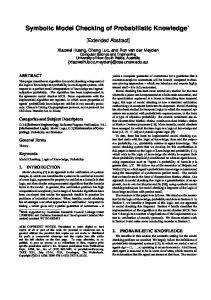
def(toss(X), pref(in(X, Y), prob_choice([pref(tau(p), pref(out(Y, head), zero)), pref(tau(1-p), pref(out(Y, tail), zero))]))). | ?- stg(toss(try)).

The definition of trans is shown in Fig. 3. The predicates prob branch, set par steps and set nu steps are defined to construct the list PSteps according to the operational semantics rules P ROB, PAR and R ES. Other auxiliary predicates used in Fig. 3 are given in Fig. 4. Note the close correspondence between the definitions in Fig. 3 and the rules of the symbolic semantics in Fig. 1. The soundness and completeness of the encoding can be established by induction on the length of derivations of a query answer of trans and a symbolic transition in πprob , respectively. The proof details are similar to Theorems 2 and 3 in [10]. Finally, we add an extra XSB predicate stg(P), which uses query-evaluation on trans to derive the PSTG of process P and output it in a simple textual format. This is done through a depth-first traversal of the graph, followed by an enumeration of all its symbolic states and transitions. The XSB code for this can be found in [30]. Example: Consider the simple πprob process T oss: T oss(x) , x(y). pτ.¯ y head.0 ⊕ (1 − p)τ.¯ y tail.0

which receives a name y on channel x and then sends out, on channel y, either head or tail, with probability p or 1−p, respectively. Fig. 5 shows the application of MMCprob to the process T oss. The first four lines illustrate the encoding of the πprob syntax into XSB. Below that is the output of the tool, i.e. the application of the rule stg. Lines starting #i show the πprob term for the ith state, lines starting ∗j and 0 k enumerate transitions and the individual edges of transitions, respectively. All bound names are given unique names (e.g. h417) and displayed on lines beginning >. All free names used are listed at the end, plus other statistics for the PSTG.

#1: proc(toss(try)) *1: 1 == #2: prob_choice([pref(tau(p),pref(out(_h417,head), zero)),pref(tau(1-p),pref(out(_h417,tail),zero))]) >1: _h417 ’1: -- ’1’:in(try,_h417) --> 2 *2: 2 == #3: pref(out(_h417,head),zero) ’2: -- ’p’:tau --> 3 #4: pref(out(_h417,tail),zero) ’3: -- ’1 - p’:tau --> 4 *3: 3 == #5: zero ’4: -- ’1’:out(_h417,head) --> 5 *4: 4 == ’5: -- ’1’:out(_h417,tail) --> 5 [1: try] [2: head] [3: tail] +++ Statistics of toss(try) +++ Nodes:5, Edges:5, P-Steps:4, Free Names:3, Bound Names:1

Fig. 5.

Sample output from MMCprob

The stochastic case: The generation of the SSTG for a πstoc process proceeds in almost identical fashion. Since the calculus has no probabilistic choice operator, the list PSteps in the representation trans(P, PSteps, M) of each symbolic transition contains only a single item of the form pstep(ri , act, Pi ), where ri now represents a real-valued rate, instead of a probability. The encoding of a rate-labelled prefix process τr .P is treated as a special case of the probabilistic choice operator for πprob with a singleton operand. Input and output actions over a channel x are given dummy rates of 1 which will be replaced with the channel rate rate(x) subsequently. Since MMCprob simply enumerates all matching transitions when evaluating the symbolic semantics (and does not remove any duplicates), no special treatment is required to deal with the multi-relation in the definition of SSTGs.

8



IV. T RANSLATING PSTG S AND SSTG S INTO PRISM We use the probabilistic model checker PRISM (which supports both MDPs and CTMCs) to perform analysis of the semantic models derived from πprob or πstoc processes. The scheme described in the previous section can be used to translate an arbitrary process described in either the simple probabilistic π-calculus or stochastic π-calculus into the probabilistic or stochastic symbolic transition graph representing its semantics. We apply model checking to closed processes (this issue is discussed further in Section IV-F), for which the symbolic (PSTG or SSTG) semantics and concrete (MDP or CTMC) semantics coincide. The list of states and transitions produced by MMCprob , as illustrated by the example in Fig. 5, can hence easily be imported directly into PRISM for analysis. However, for processes of a specific structure, we instead propose to adopt a compositional translation, using the highlevel modelling language supported by PRISM. This results in a much more efficient translation procedure. More specifically, we consider the case where systems are of the form P = νx1 . . . νxk (P1 | · · · | Pn ) and each Pi contains no instances of the ν operator (including inside recursive definitions). The basic idea is to generate the symbolic transition graph for each subprocess Pi (as described in the previous section), map each individual symbolic transition graph to a PRISM module (a component of a PRISM language model), and then use PRISM to construct the semantics of P through the parallel composition of these modules. Note that the compositional nature of this approach is reliant on our use of symbolic semantics. Without this, we would not be able to generate the full semantics of Pi in isolation. The overall process structure we impose (a parallel composition of a set of processes, optionally enclosed inside a restriction of one or more names) is actually fairly typical: systems are generally modelled as a parallel composition of multiple components and, since we assume that P is closed, it is likely that free names used as channels between processes will be restricted in this way. Furthermore, in most cases a process can be rearranged to a structurally congruent process which is of the correct form, by pushing ν operators to the outside. We have, for example, that P1 | νx P2 and νx (P1 | P2 ) are structurally congruent under the assumption that x does not occur in P1 . The only class of processes which cannot be renamed in this way are those that include ν inside recursive definitions. In this case, the process can in principle generate an infinite number of new names. This can be resolved in the context of a parallel composition with other processes, and therefore in such a case we can resort to the basic approach: use MMCprob to construct the symbolic transition graph for the full system and import this directly into PRISM. There are two principal challenges regarding the translation of symbolic transition graphs into PRISM: (1) mapping the name datatype into PRISM’s basic type system; and (2) mapping binary (CCS-style) communication of names over channels to PRISM’s multi-way (CSP-style) synchronisation without value passing. In brief, (1) is handled by enumerating the set of all free names, assigning each an (identically named) integer constant to represent it, and (2) is handled by introduc-

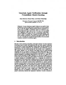
ing an action label for each required combination of process sender/receiver pair, channel and name. Communication of names between processes is handled by including in each receiver process with a bound input variable x, an identically named local (integer) variable which will be used to store the name assigned to x. Before discussing the details of this compositional translation, we give both an overview of the PRISM syntax and semantics and a simple example which illustrates the key aspects of the translation. A. PRISM semantics A PRISM model comprises a set of n modules, the state of each being given by a set of finite-ranging local variables. The global state of the model is determined by the union of all local variables, which we denote V . The behaviour of each module is defined by a set of guarded commands. When modelling MDPs, these commands take the form: [act] guard → p1 : u1 + · · · + pm : um ; where act is an (optional) action label, guard is a predicate over V , pi ∈ (0, 1] and ui are updates of the form: (x01 =ui,1 ) & . . . & (x0k =ui,k ) where ui,j is a function over V . Intuitively, in global state s of the PRISM model, the command is enabled if s satisfies guard . If a command is executed, the module will, with probability pi update its local variables according to the update ui , by setting the value of each local variable xj to ui,j (s). When modelling CTMCs, commands are of the form: [act] guard → r : u; where act is an (optional) action label, guard is a predicate over V , r ∈ R>0 and u is an update (of the form shown above). In this case, when the guard is satisfied, there is a transition with rate r that updates the local variables according to u. When multiple commands with the same update are enabled, the corresponding transitions are combined into a single transition whose rate is the sum of the individual rates. In practice (see for example Fig. 6), we omit probabilities (or rates) equal to one and elements of updates that are of the form (x0 =x). The semantics of the whole PRISM model is the parallel composition of all modules using the standard CSP parallel composition [31] (i.e. modules synchronise over all their common actions). For transitions arising from synchronisation between multiple processes, the associated probability or rate is obtained by multiplying those of each component transition. See [32] for the full semantics of the PRISM language. B. Example Translation Consider the following parallel composition of two processes expressed in the simple probabilistic π-calculus: • Q , νa (Q1 | Q2 ) 1 • Q1 , νc νd 2 τ.¯ ac.c(v).0 ⊕ 21 τ.¯ ad.d(w).0 • Q2 , νb a(x).¯ bx.0 | b(y).¯ y e.0

NORMAN et al.: MODEL CHECKING PROBABILISTIC AND STOCHASTIC EXTENSIONS OF THE π-CALCULUS const int a = 1; const int b = 2; const int c = 3; const int d = 4; const int e = 5; module P1 s1 : [1..6] init 1; v : [0..5] init 0; w : [0..5] init 0; [] (s1 = 1) → 0.5 : (s10 = 2) + 0.5 : (s10 = 3); [a P1 P2 c] (s1 = 2) → (s10 = 4); [a P1 P2 d] (s1 = 3) → (s10 = 5); [c P3 P1 e] (s1 = 4) → (s10 = 6); & (v 0 = e) [d P3 P1 e] (s1 = 5) → (s10 = 6); & (w 0 = e) endmodule module P2 s2 : [1..3] init 1 x : [0..5] init 0; [a P1 P2 c] (s2 = 1) → (s20 = 2) & (x 0 = c); [a P1 P2 d] (s2 = 1) → (s20 = 2) & (x 0 = d); [b P2 P3 x ] (s2 = 2) → (s20 = 3); endmodule module P3 s3 : [1..2] init 1 y : [0..5] init 0; [b P2 P3 x ] (s3 = 1) → (s30 = 2) & (y 0 = x ); [c P3 P1 e] (s3 = 2) & (y = c) → (s30 = 3); [d P3 P1 e] (s3 = 2) & (y = d) → (s30 = 3); endmodule

1. 2. 3. 4. 5. 6. 7. 8. 9. 10. 11. 12. 13. 14. 15. 16. 17. 18. 19. 20. 21. 22. 23. 24. 25. 26.


Fig. 6.

PRISM code for the example

Process Q1 includes two names c and d, available only within the scope of Q1 , representing private channels. It makes a random choice, outputting with equal probability either the name c or d on channel a. It then attempts to receive an input on the corresponding channel (c or d, respectively) and terminates. Process Q2 is the parallel composition of two subprocesses which communicate over a channel b. The first subprocess inputs a name on channel a (which will be one of the two private channels from Q1 ) and re-outputs it on channel b. The second subprocess inputs on channel b and then outputs e on whichever channel it received. Noting that c and d do not occur in Q2 and that b does not occur in Q1 , we can rewrite Q as the structurally congruent process P , defined as follows: • P , νa νb νc νd (P1 | P2 | P3 ) 1 ac.c(v).0 ⊕ 21 τ.¯ ad.d(w).0 • P1 , 2 τ.¯ • P2 , a(x).¯ bx.0 • P3 , b(y).¯ y e.0 and the corresponding PSTGs are given by: •

τ

a ¯c

c(v)

P1 : Q11 − → {| 12 :Q12 , 12 :Q13 |}, Q12 −→ Q14 −−→ Q16 and a ¯d

d(w)

Q13 −→ Q15 −−−→ Q16 •

¯ bx

a(x)

P2 : Q21 −−−→ Q22 −→ Q23 b(y) Q31 −−→

y¯e Q32 −→

P3 : Q33 In the above, we omit probabilities that are 1 and conditions true. The PSTGs for P1 , P2 and P3 have the sets of bound names {v, w}, {x} and {y}, respectively, and the combined set of free names is {a, b, c, d, e}. The resulting PRISM model is shown in Fig. 6. This example will be referred to in the full explanation of the translation given below. •

9

For clarity, we will retain wherever possible identical notation between the π-calculus terms and the resulting PRISM language description. Thus, each of the n subprocesses (or symbolic transition graphs) Pi becomes a PRISM module Pi and the (finite) set of terms Si = {Qi1 , . . . , Qiki } that constitute states of the symbolic transition graph of Pi becomes a set of integer indices Qi1 , . . . , Qiki uniquely representing each one. Module Pi has |Nibn | + 1 local variables: its local state (i.e. the state of the corresponding symbolic transition graph) is represented by variable si , with range Qi1 , . . . , Qiki , and each bound name xij ∈ Nibn has a corresponding variable xij with range 0, . . . , |N fn |. The model also includes |N fn | integer constants, one for each free name, which are assigned (in some arbitrary order) distinct, consecutive non-zero values. If the value of variable xij is equal to one of the these constants, then the corresponding bound name has been assigned the appropriate free name (by an input action). If xij =0, no input to the bound name has occurred yet. In this way, the conditions which label transitions of the symbolic transition graph can be translated directly into PRISM. For example, if condition M equals [x=a]∧[y=b] where x, y are bound names and a, b free names, then the translation of M into PRISM is identical: (x=a)&(y=b), where x, y are integer variables and a, b integer constants. In addition, when translating stochastic π-calculus processes, for each free name x we add to the PRISM description a constant rate x whose value is equal to rate(x), i.e. the rate associated with the channel x. For each transition in the symbolic transition graph for Pi , we will include a set of corresponding PRISM commands in the module Pi . We consider each type of transition separately below. Note that, if Pi is a simple probabilistic π-calculus term, then from the semantics (see Fig. 1) the only transitions which can include multiple probabilistic choices are internal, therefore the remaining types of transitions (input and M,α output) can be written in the simplified form Qi −−−→ Ri . For the stochastic case, since PRISM multiplies the rates of synchronising transitions and synchronisation in the π-calculus is always binary, we associate rates (e.g. rate x for channel x) with the “output” transitions and set the rates for “input” transitions to 1 (which is the default so can be omitted). Case 1 (probabilistic internal transition). For a transition: M,τ

i Qi −−−→ {|p1 : R1i , . . . , pm : Rm |}

we add the command: i [] (si =Qi ) & M → p1 :(si0 =R1i ) + · · · + pm :(si0 =Rm );

See Fig. 6 line 7 for an example. Case 2 (stochastic internal transition). For a transition: M,r

Qi −−→ Ri C. Formal translation We assume that the set of all names in the system is N , which is partitioned into disjoint subsets: N fn , the set of all free names appearing in processes P1 , . . . , Pn , and N1bn , . . . , Nnbn , the sets of input-bound names for processes P1 , . . . , P n .

we add the command: [] (si =Qi ) & M → r : (si0 =Ri ); Case 3 (output on free name). For a transition: M,¯ xy

Qi −−−→ Ri where x ∈ N fn

10


when translating simple probabilistic π-calculus processes we add, for each j ∈ {1, ..., n}\{i}, the command: [x Pi Pj y] (si =Qi ) & M → (si0 =Ri ); while for stochastic π-calculus processes we add, for each j ∈ {1, ..., n}\{i}: [x Pi Pj y] (si =Qi ) & M → rate x : (si0 =Ri ); The channel x, sender Pi , receiver Pj and sent name y are all encoded in the action label. See Fig. 6 lines 8 and 18 for examples of sending free and bound names y, respectively. Case 4 (output on bound name). For a transition: M,¯ xy

Qi −−−→ Ri where x ∈ Nibn in the probabilistic case we add, for each a ∈ N fn and j ∈ {1, ..., n}\{i}:


[a Pi Pj y] (si =Qi ) & M & (x=a) → (si0 =Ri ); while, in the stochastic case, for each a ∈ N fn and j ∈ {1, ..., n}\{i} the command: [a Pi Pj y] (si =Qi ) & M & (x=a) → rate a : (si0 =Ri ); is added. This is similar to Case 3 except that we include a command for each possible value a of x. See for example lines 24 and 25 of Fig. 6. Case 5 (input on free name). For a transition: M,x(z)

Qi −−−−→ Ri where x ∈ N fn in both cases we add, for each y ∈ N \Nibn and j ∈ {1, ..., n}\{i}, the command: [x Pj Pi y] (si =Qi ) & M → (si0 =Ri ) & (z 0 =y); For input actions, we add a line for each possible received name y. The assignment (z 0 =y) models the update of the bound name z to y. See for example lines 16 and 17 of Fig. 6 which match the output commands from lines 8 and 9. Notice that this translation also works in the case where y is a bound name in another process Pj (see for example line 23 of Fig. 6). Case 6 (input on bound name). For a transition: M,x(z)

Qi −−−−→ Ri where x ∈ Nibn when translating both simple probabilistic and stochastic processes, we add for each a ∈ N fn , y ∈ N \Nibn and j ∈ {1, ..., n}\{i} the command: [a Pj Pi y] (si =Qi ) & M & (x=a) → (si0 =Ri ) & (z 0 =y); This case combines elements of Cases 4 and 5: we add a command for each possible pairing of channel a that x may represent and name y that may be received. Finally, we need to remove some spurious commands added in Cases 5 and 6, since they correspond to input actions which will never occur. More precisely, for each module Pj we identify labels x Pi Pj y which appear on a command of Pj but which do not appear in any of the commands in module Pi . Commands with such action labels are removed from Pj .

For example, in Fig. 6 since process P1 only outputs c or d on channel a, there is no label of the form a P1 P2 e in module P1 , and therefore commands with this label have been removed from module P2 . D. Correctness of the translation By assumption, the term being translated is finite control, is closed and of the form P = νx1 . . . νxk (P1 | · · · | Pn ). The first step in the proof is to show that any term in the derivation tree of P is of the form νx1 . . . νxk (Q1 σ1 | · · · | Qn σn ) where, for any 1≤j≤n, Qj is a state of the symbolic transition graph for the process Pj and σj is a substitution from the bound names of Pj to the free names of P1 , . . . , Pn . The proof is by induction on the (concrete) transition rules using Lemma 1 or Lemma 2, depending on whether we are considering πprob or πstoc . Using this result, we now show that the translation is correct by constructing a mapping between these terms and the states of the PRISM model and demonstrating that, for any term in the derivation tree of P , there is a transition in the (concrete) semantics if and only if the corresponding PRISM state has a matching transition. For any term νx1 . . . νxk (Q1 σ1 | · · · | Qn σn ) the state in the PRISM model is constructed as follows: for any 1 ≤ j ≤ n, the values of the variables of module Pj are given by sj =Qj , xj1 =ij1 , . . . , xjkj =ijkj where if σ(xjl )=z ∈ N fn , then ijl is the integer constant corresponding to the free variable z and otherwise (i.e. σ(xjl )=xjl ) ijl equals 0. The remainder of the proof is dependent on whether we are in the probabilistic or stochastic setting. 1) Probabilistic case: Consider any πprob term Q in the derivation tree, where Q = νx1 . . . νxk (Q1 σ1 | · · · | Qn σn ) τ and the transition Q − → {|pm : Rm |}m . From the transition rules and the conditions we have imposed on the structure of πprob terms, there are the following two cases to consider. τ

0

j |}m and → {|pm : Rm Internal transition. Qj σj − j0 Rm = νx1 . . . νxk (Q1 σ1 | · · · | Rm | · · · | Qn σn ). From Mj ,τ

j Lemma 1(b), we have Qj −−−→ {|pm : Rm |} where σj |= Mj j j0 and Rm σj = Rm . Hence, by construction in the module Pj there is a command of the form: j [] (sj =Qj ) & Mj → p1 :(sj0 =R1j ) + · · · + pm :(sj0 =Rm );

Finally, since σj |= Mj and by definition of the mapping between πprob terms and PRISM, it follows that the PRISM state corresponding to Q satisfies the guard (sj =Qj ) & Mj and that the transition is preserved in the translation. x(z)

x ¯y

Communication. Qj σj −−−→ Rj0 , Ql σl −→ Rl0 , j 6= l, and {|pm : Rm |}m = {|1 : R|} where R = νx1 . . . νxk (Q1 σ1 | · · · | Rj0 {y/z} | · · · | Rl0 | · · · | Qn σn ). From Lemma 2(b), assuming without loss of generality that z is fresh: Mj ,xj (zj ) • Qj −−−−−−→ Rj where σj |=Mj and (xj (zj ).Rj )σj = x(z).Rj0 ; •

Ml ,¯ xl yl

Ql −−−−−→ Rl where σl |=Ml and (¯ xl yl .Rl )σl = x ¯y.Rl0 .


Now, since z is fresh, it follows that z=zj and, because σl is a substitution from bound to free names of P1 , . . . , Pn , it follows that y ∈ N \Njbn . In addition, since σj is a substitution from bound to free names, either xj is free and equals x, and hence in module Pj we have the command: [x Pl Pj y] (sj =Qj ) & Mj → (sj0 =Rj ) & (zj0 =y); or xj is bound and, since xj σj = x, it follows that x is free, and therefore the command: [x Pl Pj y] (sj =Qj ) & Mj & (xj =x) → (sj0 =Rj ) & (zj0 =y); appears in module Pj . Employing similar arguments, if xl is free, then xl = x and the command: [x Pl Pj y] (sl =Ql ) & Ml → (sl0 =Rl ); appears in module Pl . While, if xl is bound, then module Pl includes the command:


[x Pl Pj y] (sl =Ql ) & Ml & (xl =x) → (sl0 =Rl ); Since σj |= Mj , σl |= Ml , xj σj = x and xl σl = x, it follows that the guards (sj =Qj ) & Mj , (sj =Qj ) & Mj & (xj =x), (sl =Ql ) & Ml and (sl =Ql ) & Ml & (xl =x) hold in the PRISM state encoding Q. Finally, since the encoding of Rj0 {y/z} can be obtained from the encoding of Rj σj by setting the variable z to value y, it follows that the transition is preserved by the translation. To complete the proof it remains to show that for any transition of the PRISM model there is a matching transition in the corresponding πprob term. The result follows in a similar manner to the above using Lemma 1(a) instead of Lemma 1(b). 2) Stochastic case: Consider any πstoc term Q in the derivation tree, where Q = νx1 . . . νxk (Q1 σ1 | · · · | Qn σn ) and the r transition Q − → νx1 . . . νxk R. From the transition rules and the conditions we have imposed on the structure of πstoc terms, there are the following two cases to consider. r

= Internal transition. Qj σj − → Rj0 and R 0 Q1 σ1 | · · · | Rj | · · · | Qn σn . From Lemma 2(b), we have Mj ,r

Qj −−−→ Rj where σj |= Mj and Rj σj = Rj0 . Hence, by construction in the module Pj there is a command of the form: [] (sj =Qj ) & Mj → r : (sj0 =Rj ); Finally, since σj |= Mj and by definition of the mapping between πstoc terms and PRISM, it follows that the PRISM state corresponding to Q satisfies the guard (sj =Qj ) & Mj and that the transition is preserved in the translation. x(z)

x ¯y

Communication. Qj σj −−−→ Rj0 , Ql σl −→ Rl0 , j 6= l, R = Q1 σ1 | · · · | Rj0 {y/z} | · · · | Rl0 | · · · | Qn σn and rate(x) = r. From Lemma 2(b), assuming without loss of generality that z is fresh: •

•

Mj ,xj (zj )

Qj −−−−−−→ Rj where σj |=Mj and (xj (zj ).Rj )σj = x(z).Rj0 ; Ml ,¯ xl yl

Ql −−−−−→ Rl where σl |=Ml and (¯ xl yl .Rl )σl = x ¯y.Rl0 .

11

We employ the same arguments used in the probabilistic case. If xj is free, module Pj contains the command: [x Pl Pj y] (sj =Qj ) & Mj → (sj0 =Rj ) & (zj0 =y); while if xj is bound, it contains the command: [x Pl Pj y] (sj =Qj ) & Mj & (xj =x) → (sj0 =Rj ) & (zj0 =y); Similarly, if xl is free, the command: [x Pl Pj y] (sl =Ql ) & Ml → rate x : (sl0 =Rl ); appears in module Pl and, if xl is bound, then the command: [x Pl Pj y] (sl =Ql ) & Ml & (xl =x) → rate x : (sl0 =Rl ); appears in module Pl . The remaining arguments are the same as in the probabilistic case, using additionally the fact that the PRISM constant rate x has been given the value rate(x). E. Optimisations The translation from symbolic transition graphs to PRISM code described in this section can be optimised to reduce the size of the generated code and the resulting model. The basic idea is to compute an over-approximation of the possible values that each symbolic transition graph’s bound name can take and, thus, the channels it can send out on and the values that can be sent on those channels. With this information, we can decrease the range of the PRISM local variables corresponding to each bound name and remove unnecessary commands corresponding to combinations of channel, value and processes that can never occur. The over-approximation is computed iteratively, starting with an empty set of possible values for each bound name, and at each step adding any name that can be received upon any channel that can be used to assign to the bound name. The iterations required is bounded by the number of processes n. For clarity of presentation, the example in Fig. 6 has in fact been optimised in this way. This optimisation could be improved by employing more complex techniques based on those developed in [18] which use control flow analysis to establish an over-approximation of the set of channels a name may be bound to and the set of names that may be sent along a given channel. F. Properties For probabilistic model checking of MDPs and CTMCs, properties are typically specified using the temporal logics PCTL [33], [34] and CSL [35], [36], the key components of which are timed and untimed probabilistic reachability. Examples of expressible properties include the maximum probability of a failure occurring (Pmax=? [F failure]), the minimum probability of a process successfully completing (Pmin=? [F success]), the probability that a message is delivered by time t(∈ R) (P=? [F≤t delivered ]) and the probability of a reaction occurring in the time interval [t1 , t2 ](⊆ R) (P=? [F[t1 ,t2 ] reaction]). In practice, a wide range of useful properties can be expressed in this way.


12


Most probabilistic model checking tools, including PRISM, use state-based property specifications, i.e. the atomic propositions (failure, delivered , etc.) in the examples above are quantifier-free predicates identifying a set of states in the model. Also, the models that are checked are closed: there are no inputs/outputs between the model and its environment, only between components included within the model. This is our reason for only performing probabilistic model checking on closed π-calculus processes. In terms of the translation from π-calculus description to PRISM model, we simply need to be able to identify the particular set of target states specified in the reachability property. This is done through the MMCprob translator when it constructs a PSTG or SSTG: either by identifying which symbolic states correspond to a particular process term; or those in which a particular action is available (in the latter case, such actions can be added purely for the purposes of identifying states, and then removed through restriction). For example, consider a distributed randomised algorithm executed between n parallel components, P1 , . . . , Pn . A typical property to be checked is that algorithm always terminates with probability 1 (for any possible scheduling of the n components). In this case, we would identify the term in the π-calculus description of each process Pi that corresponds to that process finishing its execution of the algorithm. From the output of the MMCprob translator, we can identify the corresponding local state Qi of the process. We would then compute (in PRISM) the (minimum probability) of reaching the state s1 = Q1 ∧ · · · ∧ sn = Qn . Although not considered in the case studies used in this paper, our implementation could also be extended to allow for the computation of cost- or reward-based properties, which are also supported by PRISM. This allows expression of properties such as the “maximum expected number of messages sent before termination” or “the minimum expected power consumption within t time units”. Typically the cost/reward information needed for these properties is added to the model (MDP or CTMC) by annotating either transitions labelled with particular actions (for example the action-label which corresponds to a message being sent between two components) or states with real values. Since our translation of the probabilistic or stochastic π-calculus to PRISM preserves both information about the state and channel communications of a process, information of this kind could be incorporated into the translation in a relatively straightforward fashion. More general temporal properties, for example that a certain sequence of actions is performed, could be encoded through the addition of a test/watchdog process [37]. Model checking for specification formalisms more specifically tailored to the mobile aspects of the π-calculus, such as spatial logic [38], will be an area of future work. V. I MPLEMENTATION AND RESULTS Our implementation of model checking for the simple probabilistic π-calculus and stochastic π-calculus is fully automated and comprises three parts: (1) MMCprob , an extension of MMC (as described in Section III), which constructs the sym-

bolic transition graphs for a simple probabilistic or stochastic π-calculus process, (2) the translator from the symbolic transition graph to PRISM code (as described in Section IV), implemented in Java, and (3) the probabilistic model checker PRISM [11] which builds the MDP/CTMC from part (2) and performs verification of PCTL/CSL properties. We based our implementation on MMC 1.0 and PRISM 3.1.1. Firstly, we consider the dining cryptographers protocol (DCP) [39], Chaum’s randomised solution to the classic anonymity problem in which a group of N parties collectively establish whether either one of the group or an independent party has to make a payment. If the former, this is achieved without any of the N −1 non-paying parties knowing the identity of the paying one. This was previously modelled in the probabilistic π-calculus in [6]. To check anonymity, we compute the probability of reaching each of the possible outcomes of the protocol (from the point of view of an individual party) and establish that they are identical. Secondly, we study the partial secret exchange (PSE) algorithm of [3] for anonymous contract signing between two parties. A probabilistic π-calculus model of PSE was given in [5]. The protocol was independently analysed in PRISM [40], where a potential flaw of the protocol was identified, in that one party always has an advantage over the other. Several modifications to the protocol were proposed and shown to have a lower probability of this occurring. We used a πprob model of both the original and a modified version to demonstrate the same flaw. Thirdly, we constructed both a probabilistic and stochastic model of a mobile communication network (MCN), based on the (non-probabilistic) π-calculus model in [41]. The system comprises N base stations with fixed communication links to a mobile switching centre and a mobile station which can be connected to each of the base stations via radio links. The mobile station roams between the base stations. When it changes base station, the mobile communication network acts as an intermediate party, controlling the handover protocol and exchange of communication links between stations. This case study was analysed using MMC in [10]. In both this and the original paper, though, the occurrence of a failure during the handover protocol was modelled as a nondeterministic choice. In the probabilistic version we are able to correctly model this as a random event. For the stochastic model, we used the adapted version of [42]. This allows both correct modelling of the failure event and also timing characteristics of the network. We check the probability of a handover operation completing successfully, within a given number of communications (for the probabilistic case) or within a fixed time deadline (for the stochastic case). Our final case study is a CTMC model of the Fibroblast Growth Factor (FGF) signalling pathway. We consider a slightly simplified version of the model from [43], comprising interactions between a mixture of FGF ligands and receptors. In the πstoc formulation, the ν operator is used to give each FGF ligand a unique channel name. The binding between a particular FGF ligand and receptor is modelled by this name being passed between the two. Unbinding occurs through a communication over this private channel. We check the


13

TABLE I P ERFORMANCE OF THE PROBABILISTIC MODEL CHECKING PROCESS


Case study

N States

Model size Transitions

MTBDD size (nodes)

Construction time (sec.) PSTGs/ PRISM MDP/ SSTGs code CTMC

Model checking in PRISM (sec.)

DCP

5 6 7 8 9

160,543 1,475,401 13,221,889 116,192,457 1,005,495,499

592,397 6,520,558 68,121,834 683,937,352 6,657,256,911

58,448 100,122 154,074 220,043 298,285

2.20 2.50 2.95 3.31 3.62

0.27 0.27 0.31 0.31 0.36

0.93 1.98 3.10 4.23 6.26

5.21 15.1 39.4 90.8 316.2

PSE

3 4 5

9,321 89,025 837,361

32,052 419,172 5,028,700

17,999 43,120 88,074

1.63 2.12 2.60

0.21 0.27 0.31

0.43 0.95 1.89

0.31 1.23 2.96

PSEmod

3 4 5

9,328 89,040 837,392

32,059 419,187 5,028,731

18,184 43,388 89,309

1.57 1.99 2.49

0.22 0.26 0.31

0.41 0.89 1.96

0.86 3.45 14.3

MCN (probabilistic)

2 3

609 3,611

950 5,811

58,430 216,477

1.38 1.60

0.31 0.46

2.61 12.0

0.34 6.06

MCN (stochastic)

2 3

565 3,295

854 5,079

32,898 119,197

1.44 1.59

0.38 0.44

2.13 7.05

1.18 2.76

3 4 5 6

13,081 87,109 453,593 2,011,729

43,330 315,436 1,763,842 8,318,684

8,667 28,725 108,354 304,464

1.00 1.08 1.21 1.39

0.11 0.12 0.12 0.16

0.25 1.34 8.62 32.3

2.22 24.1 156.6 999.3

FGF

probability that all FGF receptors have relocated (are no longer active) by a certain time bound. Table I shows the performance of our implementation on the case studies. Experiments were run on a 2 GHz PC with 2 GB RAM running Linux. For each case study, we analysed several models of increasing size by varying a parameter N . For the DCP model, N represents the number of parties; for PSE (we consider two variants: the original protocol EGL and the modified version EGL3 from [40]) N is the size of contract; for the MCN models, N represents the number of base stations; and for FGF, N is the number of FGF ligands (the number of receptors remains fixed). The table shows the size of the resulting MDPs/CTMCs (number of states/transitions) and corresponding storage in PRISM (MTBDD nodes, where 1 node uses 20 bytes). We also give the time required for each stage of the process, i.e. constructing: the PSTGs (using MMCprob ); the PRISM code (using the translator); and the MDP or CTMC model (using PRISM). Finally, we give the time to check a single (quantitative) PCTL/CSL property for each using PRISM (with the fastest available engine). The results are very encouraging. We see that our techniques are scalable to the construction and analysis of πprob and πstoc models with extremely large state spaces and that the times required for all stages of the process are relatively small. Furthermore, the compositional approach to the translation proved to be essential. On the FGF model (N =3), for example, constructing the full model in MMCprob took more than 100 times as long as the compositional technique. For larger parameter values, it was not feasible to directly construct the full model. The MCN case study, although smallest in terms of state space, is a particularly good example of the applicability of this implementation since it fully exploits all mobile aspects of the calculus. The most obvious area for improvement in

our results concerns MTBDD sizes. As is often the case with automatically generated code, the PRISM models resulting from our technique do not always exhibit the kind of structure and regularity that can be exploited by PRISM’s symbolic implementation. We are confident that performance can be improved in this area.

VI. C ONCLUSIONS In this paper we have demonstrated the feasibility of implementing model checking for probabilistic and stochastic extensions of the π-calculus. Furthermore we have shown, through its application to several large examples, the efficiency of the approach. The probabilistic version of the π-calculus we used (with only blind probabilistic choice) has proved to be expressive enough for the appropriate application domains (probabilistic algorithms for security and dynamic communication protocols with failures and/or randomisation) and yet amenable to analysis with extensions and adaptions of existing verification tools. Similarly, the version of the stochastic πcalculus we used (with rates assigned to τ transitions and to channels) is both a natural formalism for modelling biological systems and well suited for the model checking techniques we have proposed. We would like to extend this work in several directions. For convenience of modelling, we plan to add support for polyadic communication over channels. We also hope to add support for more flexible property specifications using watchdog processes. Finally, we will investigate ways to further improve the efficiency of our implementation, in particular, with regards to the automatically generated PRISM code. Possibilities include optimisations to reduce the resulting symbolic (MTBDD) storage in PRISM and bisimulation minimisation techniques.

14


ACKNOWLEDGMENTS Authors Norman and Parker were in the School of Computer Science at the University of Birmingham and Wu was at CNRS and LIX when parts of this work were first carried out. Norman and Parker are supported in part by EPSRC grants GR/S11107 and GR/S46727 and Microsoft Research Cambridge contract MRL 2005-44 and Palamidessi and Wu were supported in part by the INRIA/ARC project ProNoBis. We thank the anonymous referees for their valuable comments.


R EFERENCES [1] R. Milner, J. Parrow, and D. Walker, “A calculus of mobile processes, I,” Information and Computation, vol. 100, pp. 1–40, 1992. [2] M. Reiter and A. Rubin, “Crowds: Anonymity for web transactions,” ACM Transactions on Information and System Security, vol. 1, no. 1, pp. 66–92, 1998. [3] S. Even, O. Goldreich, and A. Lempel, “A randomized protocol for signing contracts,” Communications of the ACM, vol. 28, no. 6, pp. 637–647, 1985. [4] O. Herescu and C. Palamidessi, “Probabilistic asynchronous π-calculus,” in Proc. 3rd Int. Conf. Foundations of Software Science and Computation Structures (FOSSACS’00), ser. Lecture Notes in Computer Science, J. Tiuryn, Ed., vol. 1784. Springer, 2000, pp. 146–160. [5] K. Chatzikokolakis and C. Palamidessi, “A framework to analyze probabilistic protocols and its application to the partial secrets exchange,” in Proc. Int. Symp. Trustworthy Global Computing (TGC’05), ser. Lecture Notes in Computer Science, R. D. Nicola and D. Sangiorgi, Eds., vol. 3705. Springer, 2005, pp. 146–162. [6] M. Bhargava and C. Palamidessi, “Probabilistic anonymity,” in Proc. 16th Int. Conf. Concurrency Theory (CONCUR’05), ser. Lecture Notes in Computer Science, M. Abadi and L. de Alfaro, Eds., vol. 3653. Springer, 2005, pp. 171–185. [7] C. Priami, “Stochastic π-calculus,” The Computer Journal, vol. 38, no. 7, pp. 578–589, 1995. [8] A. Regev, W. Silverman, and E. Shapiro, “Representation and simulation of biochemical processes using the π-calculus process algebra,” in Pacific Symposium on Biocomputing, R. Altman, A. Dunker, L. Hunter, and T. Klein, Eds., vol. 6. World Scientific Press, 2001, pp. 459–470. [9] C. Priami, A. Regev, W. Silverman, and E. Shapiro, “Application of a stochastic name passing calculus to representation and simulation of molecular processes,” Information Processing Letters, vol. 80, pp. 25– 31, 2001. [10] P. Yang, C. Ramakrishnam, and S. Smolka, “A logic encoding of the π-calculus: model checking mobile processes using tabled resolution,” Int. Journal on Software Tools Technology Transfer, vol. 4, pp. 1–29, 2004. [11] A. Hinton, M. Kwiatkowska, G. Norman, and D. Parker, “PRISM: A tool for automatic verification of probabilistic systems,” in Proc. 12th Int. Conf. Tools and Algorithms for the Construction and Analysis of Systems (TACAS’06), ser. Lecture Notes in Computer Science, H. Hermanns and J. Palsberg, Eds., vol. 3920. Springer, 2006, pp. 441–444. [12] B. Victor and F. Moller, “The Mobility Workbench - a tool for the πcalculus,” in Proc. 6th Int. Conf. Computer Aided Verification (CAV’94), ser. Lecture Notes in Computer Science, R. Alur and D. Peled, Eds., vol. 818. Springer, 1994, pp. 428–440. [13] B. Blanchet, “ProVerif: Automatic cryptographic protocol verifier user manual,” 2005. [14] S. Chaki, S. Rajamani, and J. Rehof, “Types as models: Model checking message-passing programs,” in Proc. 29th Symp. Principles of Programming Languages (POPL’02). ACM, 2002, pp. 45–57. [15] P. Wu, “Interpreting π-calculus with Spin/Promela,” Computer Science, vol. 8, pp. 7–9, 2003, supplement. [16] H. Song and K. Compton, “Verifying π-calculus processes by Promela translation,” University of Michigan, Tech. Rep. CSE-TR-472-03, 2003. [17] A. Venet, “Abstract interpretation of the pi-calculus,” in Proc. 5th LOMAPS Workshop on Analysis and Verification of Multiple-Agent Languages, ser. LNCS, M. Dam, Ed., vol. 1192. Springer, 1996, pp. 51–75. [18] C. Bodei, P. Degano, F. Nielson, and H. R. Nielson, “Static analysis for the pi-calculus with applications to security,” Information and Computation, vol. 165, pp. 68–92, 2001.

[19] A. Phillips and L. Cardelli, “Efficient, correct simulation of biological processes in the stochastic π-calculus,” in Proc. 5th Int. Workshop Computational Methods in Systems Biology (CMSB’07), ser. Lecture Notes in Bioinformatics, M. Calder and S. Gilmore, Eds., vol. 4695. Springer, 2007, pp. 184–199. [20] G. Norman, C. Palamidessi, D. Parker, and P. Wu, “Model checking the probabilistic π-calculus,” in Proc. 4th Int. Conf. Quantitative Evaluation of Systems (QEST’07). IEEE Computer Society, 2007, pp. 169–178. [21] R. Milner, Communication and Concurrency, ser. Int. Series in Computer Science. Prentice Hall, 1989. [22] R. Segala and N. Lynch, “Probabilistic simulations for probabilistic processes,” Nordic Journal of Computing, vol. 2, no. 2, pp. 250–273, 1995. [23] M. Hennessy and H. Lin, “Symbolic bisimulations,” Theoretical Computer Science, vol. 138, pp. 353–389, 1995. [24] P. Wu, C. Palamidessi, and H. Lin, “Symbolic bisimulations for probabilistic systems,” in Proc. 4th Int. Conf. Quantitative Evaluation of Systems (QEST’07). IEEE Computer Society, 2007, pp. 179–188. [25] H. Lin, “Symbolic bisimulation and proof systems for the π-calculus,” School of Cognitive and Computer Science, University of Sussex, Tech. Rep., 1994. [26] M. Boreale and R. D. Nicola, “A symbolic semantics for the π-calculus,” Information and Computation, vol. 126, no. 1, pp. 34–52, April 10 1996. [27] H. Lin, “Complete inference systems for weak bisimulation equivalences in the pi-calculus,” Information and Computation, vol. 180, no. 1, pp. 1–29, 2003. [28] A. Ingólfsdóttir and H. Lin, “A symbolic approach to value-passing processes,” in Handbook of Processes Algebra. Elsevier, 2001, ch. 7. [29] J. Hillston, A Compositional Approach to Performance Modelling. Cambridge University Press, 1996. [30] G. Norman, C. Palamidessi, D. Parker, and P. Wu, “Translating the probabilistic π-calculus to PRISM,” School of Computer Science, University of Birmingham, Tech. Rep. CSR-07-02, 2007. [31] A. Roscoe, The theory and practice of concurrency. Prentice-Hall, 1997. [32] Online PRISM documentation www.prismmodelchecker.org/doc/. [33] H. Hansson and B. Jonsson, “A logic for reasoning about time and reliability,” Formal Aspects of Computing, vol. 6, no. 5, pp. 512–535, 1994. [34] A. Bianco and L. de Alfaro, “Model checking of probabilistic and nondeterministic systems,” in Proc. 15th Conference on Foundations of Software Technology and Theoretical Computer Science, ser. LNCS, P. Thiagarajan, Ed., vol. 1026. Springer, 1995, pp. 499–513. [35] A. Aziz, K. Sanwal, V. Singhal, and R. Brayton, “Verifying continuous time Markov chains,” in Proc. 8th Int. Conf. Computer Aided Verification (CAV’96), ser. LNCS, R. Alur and T. Henzinger, Eds., vol. 1102. Springer, 1996, pp. 269–276. [36] C. Baier, B. Haverkort, H. Hermanns, and J.-P. Katoen, “Model-checking algorithms for continuous-time Markov chains,” IEEE Transactions on Software Engineering, vol. 29, no. 6, pp. 524–541, 2003. [37] M. Goldsmith, N. Moffat, B. Roscoe, T. Whitworth, and I. Zakiuddin, “Watchdog transformations for property-oriented model-checking,” in Proc. 2th Int. Symp. Formal Methods Europe (FME’03), ser. Lecture Notes in Computer Science, K. Araki, S. Gnesi, and D. Mandrioli, Eds., vol. 2805. Springer, 2003, pp. 600–616. [38] L. Caires and L. Cardelli, “A spatial logic for concurrency (part i),” Information and Computation, vol. 186, no. 2, pp. 194–235, 2003. [39] D. Chaum, “The dining cryptographers problem: Unconditional sender and recipient untraceability,” Journal of Cryptology, vol. 1, pp. 65–75, 1988. [40] G. Norman and V. Shmatikov, “Analysis of probabilistic contract signing,” Journal of Computer Security, vol. 14, no. 6, pp. 561–589, 2006. [41] F. Orava and J. Parrow, “An algebraic verification of a mobile network,” Formal Aspects of Computing, vol. 4, pp. 497–543, 1992. [42] C. Priami, “Stochastic analysis of mobile telephony networks,” in Proc. 5th Int. Workshop on Process Algebra and Performance Modeling (PAPM’97), E. Brinskma and A. Nymeyer, Eds., 1997, pp. 145–171, technical Report TR-CTIT-97-14. Centre for Telematics and Information Technology, University of Twente. [43] J. Heath, M. Kwiatkowska, G. Norman, D. Parker, and O. Tymchyshyn, “Probabilistic model checking of complex biological pathways,” in Proc. 4th Int. Workshop Computational Methods in Systems Biology (CMSB’06), ser. Lecture Notes in Bioinformatics, C. Priami, Ed., vol. 4210. Springer, 2006, pp. 32–47.

Model checking probabilistic and stochastic extensions of the Ï-calculus

Model checking probabilistic and stochastic extensions of the Ï-calculus

Suggest Documents

Model checking the probabilistic Ï-calculus - LIX

Probabilistic Model Checking of Complex

Symbolic Model Checking of Probabilistic

MODEL CHECKING PROBABILISTIC TIMED AUTOMATA

Symbolic Model Checking of Probabilistic Knowledge - Computer ...

Probabilistic Model Checking for Games of

Significant Diagnostic Counterexamples in Probabilistic Model Checking

Distributed Symbolic Model Checking forâcalculus

Uncertain Agent Verification through Probabilistic Model-Checking

Probabilistic Model Checking for Complex Cognitive Tasks

Probabilistic Model-Checking Support for FMEA - CiteSeerX

MODEL CHECKING PROBABILISTIC PUSHDOWN AUTOMATA 1 ...

Probabilistic Model Checking for Uncertain Scenario ...

Distributed Symbolic Model Checking forâcalculus

Probabilistic Model Checking of the CSMA/CD Protocol Using PRISM ...

Probabilistic Model Checking of Deadline Properties in the IEEE 1394 ...

A Logical Encoding of the π-Calculus: Model Checking ... - CiteSeerX

Probabilistic Model Checking of the CSMA/CD Protocol Using PRISM ...

Probabilistic Model Checking of Deadline Properties in the IEEE 1394 ...

Probabilistic model checking for the quantification of DoS ... - delab-auth

Probabilistic Model Checking of the PDGF Signaling Pathway - SaToSS

Timed and Stochastic Model Checking of Petri Nets - Dipartimento di

Probabilistic model checking in practice - PRISM Model Checker

Stochastic Calculus

Model checking probabilistic and stochastic extensions of the Ï-calculus