Model Evaluation, Testing and Selection In J. Myung, Mark A. Pitt, and Woojae Kim Department of Psychology Ohio State University January 16, 2003 (Word count: 10375)
To appear in K. Lambert and R. Goldstone (eds.), Handbook of Cognition. Sage Publication Running Head: Model Evaluation and Selection All correspondence to: Dr. In Jae Myung Department of Psychology Ohio State University 1885 Neil Avenue Columbus, Ohio 43210-1222 614-292-1862 (voice) 614-292-5601 (fax)
[email protected] (email)
Model Selection and Evaluation - 2 Model Evaluation, Testing and Selection Introduction As mathematical modeling increases in popularity in cognitive psychology, it is important for there to be tools to evaluate models in an effort to make modeling as productive as possible. Our aim in this chapter is to introduce some of these tools in the context of the problems they were meant to address. After a brief introduction to building models, the chapter focuses on their testing and selection. Before doing so, however, we raise a few questions about modeling that are meant to serve as a backdrop for the subsequent material. Why Mathematical Modeling? The study of cognition is concerned with uncovering the architecture of the mind. We want answers to questions such as how decisions are made, how verbal and written modes of communication are performed, and how people navigate through the environment. The source of information for addressing these questions are the data collected in experiments. Data are the sole link to the cognitive process of interest, and models of cognition evolve from researchers inferring the characteristics of the processes from these data. Most models are specified verbally when first proposed, and constitute a set of assumptions about the structure and function of the processing system. A verbal form of a model serves a number of important roles in the research enterprise, such as providing a good conceptual starting point for experimentation. When specified in sufficient detail, verbal models can stimulate a great deal of research, as its predictions are tested and evaluated. Even when the model is found to be incorrect (which will always be the case), the mere existence of the model will have served an important purpose in advancing our
Model Selection and Evaluation - 3 understanding and pushing the field forward. When little is known about the process of interest (i.e., data are scarce), verbal modeling is a sensible approach to studying cognition. However, simply by virtue of being verbally specified, there is a limit to how much can be learned about the process. When this point is reached, one must turn from a verbal description to a mathematical description to make progress. In this regard, mathematical modeling takes the scientific enterprise a step further to gain new insights into the underlying process and derive quantitative predictions, which are rarely possible with verbal models. In the remainder of this section, we highlight some points to consider when making this transition. What is a Mathematical Model of Cognition? Although there is no single answer to this question, thinking about it can be quite instructive when evaluating one’s goals. For instance, functional equation modeling focuses on developing the most accurate description of a phenomenon. Models of forgetting (Wixted & Ebbesen, 1991) describe how retention changes over time. Similarly, “laws” of psychophysics (Gesheider, 1985) describe the relationship between a physical stimulus and its psychological counterpart (e.g., amplitude vs. loudness). Models such as these are merely quantitative redescriptions of the input-output relationship between a stimulus and a response. There is little in the function itself that represents characteristics of the underlying process responsible for the mapping (e.g., memory). Put another way, there is no content in the "black-box" (i.e., the model) that one can appeal to understand how the input was processed to lead to a particular response. Artificial neural networks that are trained to do nothing more than learn a stimulus-response relationship fall into this category as well (e.g., Gluck, 1991).1
Model Selection and Evaluation - 4 Often this type of modeling can be quite informative. For example, there have been many demonstrations in recent years showing the sufficiency of a statistical associator (i.e., artificial neural network) in learning properties of language (e.g., verb morphology, segment cooccurrences) that were previously assumed to require explicit rules (Brent, 1999; Elman et al, 1996; Joanisse & Seidenberg, 1999). However, this approach differs in important ways from a process-oriented approach to modeling, wherein a verbal model is instantiated mathematically. In processing models, theoretical constructs in the verbal model (e.g., memory, attention, activation, levels of representation) are represented in the quantitative model. There are direct ties between the two types of models. The parameters of the quantitative model are linked to mental constructs and the functional form (i.e., the mathematical equation) integrates them in a meaningful way. The quantitative model replaces, even supersedes, the verbal model, becoming a closer approximation of the cognitive process of interest. Processing models differ widely in the extent to which they are linked to their verbal form. In general, this link may be stronger for algebraic models (Nosofsky, 1986; Shiffrin & Styvers, 1997) than localist networks (Grainger & Jacobs, 1998), in large part because of the additional parameters needed to implement a network. Both types of models not only strive to reproduce behavior, but they attempt to do so in a way that provides an explanation for the cause of the behavior. This is what makes a cognitive model cognitive. Virtues and Vices of Modeling As mentioned above, the allure of modeling is in the potential it holds for learning more about the cognitive process of interest. Precise predictions can be tested about how variables should interact or the time course of processing. In essence, cognitive modeling allows one to
Model Selection and Evaluation - 5 extract more information from the data than just ordinal mean differences between conditions. The magnitude of effects and the shape of distributions can be useful information in deciding between equally plausible alternatives. Another virtue of cognitive modeling is that it provides a framework for understanding what can be complex interactions between parts of the model. This is especially true when the model has many parameters and the parameters are combined nonlinearly. Simulations can help assess how model behavior changes when parameters are combined in different ways (e.g., additively vs multiplicatively) or what type of distribution (e.g.,. normal, exponential) best approximates a response-time distribution. Work such as this will not only lead to a better understanding of the model as it was designed, but it can also lead to new insights. One example of this is when a model displays unexpected behavior, which is later found in experimental data, thereby extending the explanatory reach of the model. They are sometimes referred to as emergent properties, particularly in the context of connectionist models. Frequently, they are compelling demonstrations of the power of models (and modeling), and the necessity of such demonstrations prior to settling on a theoretical interpretation of an experimental finding. One example is provided here to illustrate this point. A central question in the field of memory has been whether memory is composed of multiple subsystems. Dissociations in performance across tasks and populations offer some of the most irrefutable evidence in favor of separate systems. In one such study, Knowlton and Squire (1993) argued that classification and recognition are mediated by independent memory systems on the basis of data showing a dissociation between the two in normal adults and amnesic individuals. Amnesiacs performed as well as normals in pattern classification, but
Model Selection and Evaluation - 6 significantly worse in old/new recognition of those same patterns. Knowlton and Squire postulated that an implicit memory system underlies category acquisition (which is intact in amnesiacs) whereas a separate declarative knowledge system (damaged in amnesiacs) is used for recognition. As compelling as this conclusion may be, Nosofsky and Zaki (1998) performed a couple of equally convincing simulations that demonstrate a single (exemplar) memory system could account for the findings. Although an exemplar model may not account for all such findings in the literature (see Knowlton, 1999: Nosofsky & Zaki, 1998), its success offers an instructive lesson: Modeling can be a means of overcoming a limitation in our own ability to understand how alternative conceptualizations can account for what seem like strong evidence against them. See Ratcliff, Speiler, and McKoon, (2000) for a similar example in the field of cognitive aging. Despite the virtues of cognitive modeling, it is not risk-free. Indeed, it can be quite hazardous. It is far too easy for one to unknowingly create a behemoth of a model that will perform well for reasons that have nothing to do with being a good approximation of the cognitive process. How can this situation be identified and avoided? More fundamentally, how should a model be evaluated? Model testing is most often post-dictive, carried out after the data were collected. Although necessary, it is a weak test of the model’s adequacy because the model may well have been developed with those very data. Far more impressive, yet much rarer, are tests in which the model’s predictions are substantiated or invalidated in future experimentation. In the absence of such work, how might tests of one or more models be carried out most productively? After a brief overview of parameter estimation, the remainder of this chapter provides some preliminary answers to these questions.
Model Selection and Evaluation - 7 Model Specification and Parameter Estimation Model as a Parametric Family of Probability Distributions From a statistical standpoint, observed data is a random sample from an unknown population, which represents the underlying cognitive process of interest. Ideally, the goal of modeling is to deduce the population that generated the observed data. A model is in some sense a collection of populations. In statistics, associated with each population is a probability distribution indexed by the model’s parameters. Formally, a model is defined as a parametric family of probability distributions. Let us use f(y|w) to denote the probability distribution function that gives the probability of observing data y = (y1,…,ym) given the model’s parameter vector w = (w1,…,wk). Under the assumption that individual observations, yi’s, are independent of one another, f(y|w) can be rewritten as a product of individual probability distribution functions, f ( y = ( y1 ,..., y m )| w) = f ( y1 | w) f ( y 2 | w) ⋅ ⋅ ⋅ f ( y m | w).
As an illustrative example, consider the Generalized Context Model (GCMcv) of categorization that describes the probability (paj) of category Cj response given stimulus Xa by the following equation (Nosofsky, 1986):
∑S
GCMcv: paj =
b∈C j
ab
∑ ∑S j ' c∈C j '
where S ab ac
1/ r q r = exp − c ∑ v k | x ak − xbk | k =1
In the equation, Sab denotes a similarity measure between two multidimensional stimuli Xa = (xa1,…,xaq) and Xb = (xb1,…,xbq), q is the number of stimulus dimensions, c (> 0) is a sensitivity parameter, vk (> 0) is an attention weight satisfying Σ vk = 1 and finally, r is the Minkowski
Model Selection and Evaluation - 8 metric parameter. Typically, the model is specified in terms of the City-block distance metric of r = 1 or the Euclidean metric of r = 2, with the rest of the parameters being estimated from data. The model therefore has q free parameters, that is, w = (c, v1 v2 …, vq-1). Note that the last attention weight, vq, is determined from the normalization constraint, Σ vk = 1 based on the first (q-1) weights. In a categorization experiment with J categories, each yi itself, obtained under condition i (i = 1,…,m), becomes a vector of J elements, yi = (yi1,…yiJ), 0 < yij < 1, where yij represents the response proportion for category Cj. Each yij is obtained by dividing the number of category responses (xij) by the number of independent trials (n) as yij = xij/n where xij = 1, 2, …,n. Note that the vector xi = (xi1,…xiJ) itself is distributed according to a multinomial probability distribution. For instance, suppose that in condition i, the task was to categorize stimulus Xa into one of three categories, C1 - C3 (i.e., J = 3). Then the probability distribution function of xi is given by f ( xi = ( xi1 , xi 2 , xi 3 )| w) =
n! p xi 1 p xi 2 pa 3 xi 3 xi 1 ! xi 2 ! xi 3 ! a1 a 2
In the equation, paj is defined earlier as a function of the parameter vector w such that pa1 + pa2 + pa3 = 1, and also, note that xi1 + xi2 + xi3 = n. The desired probability distribution function f(yi|w) in terms of yi = (yi1, yi2, yi3) is obtained simply by substituting n·yij for xij in the above equation. Finally, the probability distribution function f(y|w) for the entire set of data y = (y1,…,ym) is given as a product of individual f(yi|w)’s over m conditions. Parameter Estimation
Model Selection and Evaluation - 9 Once a model is specified with its parameters and data have been collected, the model’s ability to fit the data can be assessed. Model fit is measured by finding parameter values of the model that provide the ‘best’ fit to the data in some defined sense—a procedure called parameter estimation in statistics. For more in-depth treatment of the topic, the reader is advised to consult Casella and Berger (2002). There are two generally accepted methods of parameter estimation: Least-squares estimation (LSE) and maximum likelihood estimation (MLE). In LSE, we seek the parameter values that minimize the sum of squares error (SSE) between observed data and a model’s predictions: m
SSE ( w) =
∑ (y i =1
i
− yi , prd ( w)) 2
where yi,prd(w) denotes the model’s prediction for observation yi. Note that SSE(w) is a function of the parameter w. In MLE, we seek the parameter values that are most likely to have produced the data. This is obtained by maximizing the log-likelihood of the observed data: m
loglik( w) =
∑ ln f ( y | w) i =1
i
where ln denotes the natural logarithm of base e, the natural number. Note that by maximizing either the likelihood or the log-likelihood, the same solution is obtained because the two are monotonically related to each other. In practice, the log-likelihood is preferred for computational ease. The parameters that minimize the sum of squares error or the log-likelihood are called the LSE or MLE estimates, respectively. For normally distributed data with constant variance, LSE and MLE are equivalent in the sense that both methods yield the same parameter estimates. For non-normal data such as
Model Selection and Evaluation - 10 proportions and response times, however, LSE estimates tend to differ from MLE estimates. Although LSE is often the ‘de facto’ method of estimation in cognitive psychology, MLE is preferrable, especially for non-normal data. In particular, MLE is well-suited for statistical inference in hypothesis testing and model selection. LSE implicitly assumes normally distributed error, and hence, will work as well as MLE to the extent that the assumption is reasonable. Finding LSE or MLE estimates generally requires use of a numerical optimization procedure on computer, as it is usually not possible to obtain an analytic form solution. In essence, the idea of numerical optimization is to find optimal parameter values by making use of a search routine that applies heuristic criteria in a trial-and-error fashion iteratively until stopping criteria are satisfied. Model Evaluation and Testing Once a model is specified and its best-fitting parameters are found, one is in a position to assess the viability of the model. Researchers have proposed a number of criteria that were thought to be important for model evaluation (e.g., Jacobs & Grainger, 1994). These include three qualitative criteria (explanatory adequacy, interpretability, faithfulness) and four quantitative criteria (falsifiability, goodness of fit, simplicity/complexity, generalizability). Below we discuss these criteria one at a time. Qualitative Criteria A model satisfies the explanatory adequacy criterion if its assumptions are plausible and consistent with established findings, and importantly, the theoretical account is reasonable for the cognitive process of interest. In other words, the model must be able to do more than redescribe observed data. The model must also be interpretable in the sense that the model makes sense and
Model Selection and Evaluation - 11 is understandable. Importantly, the components of the model, especially its parameters, must be linked to psychological processes and constructs. Finally, the model is said to be faithful to the extent that the model’s ability to capture the underlying mental process originates from the theoretical principles embodied in the model, rather than from the choices made in its computational instantiation. Although we cannot over-emphasize the importance of these qualitative criteria in model evaluation, they have yet to be quantified. Accordingly, we must rely on our subjective assessment of the model on each. In contrast, the four criteria discussed next are quantifiable. Quantitative Criteria Falsifiability. This is a necessary condition for testing a model or theory, refers to whether there exist potential observations that a model cannot describe (Popper, 1959). If so, then the model is said to be falsifiable. An unfalsifiable model is one that can describe unerringly all possible data patterns in a given experimental situation. Obviously, there is no point in testing an unfalsifiable model. A heuristic rule for determining a model’s falsifiability is already familiar to us: The model is falsifiable if and only if the number of its free parameters is less than the number of data observations. This counting rule, however, turns out to be imperfect, in particular, for certain non-linear models (Bamber & van Santen, 1985). For example, they showed that Luce’s (1959) choice model is falsifiable even if its number of parameters exceeds the number of observations! To remedy limitations of the counting rule, Bamber and van Santen (1985) provides a formal rule for assessing a model’s falsifiability, which yields the counting rule as a special case. The rule states that a model is falsifiable if the rank of its Jacobian matrix is less
Model Selection and Evaluation - 12 than the number of data observations for all values of the parameters. The Jacobian matrix is defined in terms of partial derivatives as: J ij ( w) = ∂ E ( y j ) / ∂ wi (i = 1,..., k ; j = 1,..., m) where E(x) stands for the expectation of a random variable x. Goodness of Fit. A model should also provide a good description of the observed data. Goodness of fit refers to the model’s ability to fit the particular set of observed data. Examples of goodness of fit measures are the minimized sum of squares error (SSE), the mean squared error (MSE), the root mean squared error (RMSE), the percent variance accounted for (PVAF), and the maximum likelihood (ML). The first four of these, defined below, are related to one another in a way that one can be written in terms of another: MSE = SSE ( w *LSE ) / m RMSE =
SSE ( w *LSE ) / m
PVAF = 100(1 − SSE ( w *LSE ) / SST ) ML = f ( y| w *MLE ) In the equation, w *LSE is the parameter that minimizes SSE(w), that is, an LSE estimate, and SST stands for the sum of squares total defined as SST =
∑
i
( yi − y mean ) 2 . ML is the probability
distribution function maximized with respect to the model’s parameters, evaluated at w *MLE , which is obtained through MLE. Complexity. Not only should a model describe the data in hand well, but it should also do so in the least complex (i.e., simplest) way. Intuitively, complexity has to do with a model’s inherent flexibility that enables it to fit a wide range of data patterns. There seem to be at least two dimensions of model complexity, the number of parameters and the model’s functional form. The latter refers to the way the parameters are combined in the model equation. The more
Model Selection and Evaluation - 13 parameters a model has, the more complex it is. Importantly also, two models with the same number of parameters but different functional forms can differ significantly in their complexity. For example, it seems unlikely that two one-parameter models, y = x + w and y = ewx are equally complex. The latter is probably much better at fitting data than the former. It turns out that one can devise a quantitative measure of model complexity that takes into account both dimensions of complexity and at the same time is theoretically justified as well as intuitive. One example is the geometric complexity (GC) of a model (Pitt, Myung & Zhang, 2002; Rissanen, 1996) defined as: GC =
k n ln + ln ∫ dw det I ( w) 2 2π
where k is the number of parameters, n is the sample size, I(w) is the Fisher information matrix defined as I ij ( w) = − E[∂ 2 ln f ( y| w) / ∂ wi ∂ w j ], i , j = 1,..., k , and det denotes the determinant of I ij ( w) . Functional form effects of complexity are reflected in the second term of GC through I(w). How do we interpret geometric complexity? The meaning of geometric complexity is related to the number of “different” (i.e., distinguishable) probability distributions that a model can account for. The more distinguishable distributions that the model can describe by finely tuning its parameter values, the more complex it is (Myung, Balasubramanian & Pitt, 2000). For example, when geometric complexity is calculated for the following two-parameter psychophysical models, Stevens’ law ( y = w1 x w2 ) and Fechner’s logarithmic law
( y = w1 ln( x + w2 )) , the former turns out to be more complex than the latter (Pitt et al, 2002). For another measure of model complexity called the effective number of parameters, which takes
Model Selection and Evaluation - 14 into account the model’s functional form as well as the number of parameters, see Murata, Yoshizawa and Amari (1994; Moody, 1992). Generalizability. The fourth quantitative criterion for model evaluation is generalizability. This criterion is defined as a model’s ability to fit not only the observed data in hand, but also new, as yet unseen data samples from the same probability distribution. In other words, model evaluation should not be focused solely on how well a model fits observed data, but how well it fits future data samples generated by the cognitive process underlying the data. This goal will be achieved best when generalizability is considered. To summarize, these four quantitative criteria work together to assist in model evaluation and guide (even constrain) model development and selection. The model must be sufficiently complex, but not too complex, to capture the regularity in the data. Both a good fit to the data and good generalizability will ensure an appropriate degree of complexity, so that the model captures the regularity in the data. In addition, because of its broad focus, generalizability will constrain the power of the model, thus making it falsifiable. Although all four criteria are interrelated, generalizability may be the most important. It should be the guiding principle in model evaluation and selection. Why Generalizability? On the face of it, goodness of fit might seem like it should be the main criterion in model evaluation. After all, it measures a model’s ability to fit observed data, which is our only window into cognition. So why not evaluate a model on the basis of its fit? This might be all right if the data reflected only the underlying regularity. However, data are corrupted by uncontrolable, random variation (noise) due to the inherently stochastic nature of cognitive processes and the
Model Selection and Evaluation - 15 unreliable tools used to measure cognition. An implication of noise-contaminated data is that a model’s goodness of fit reflects not only its ability to capture the underlying process, but also its ability to fit random noise. This relationship is depicted conceptually in the following equation: Goodness of fit = Fit to regularity ( generalizability ) + Fit to noise (overfitting )
We are interested in only the first term on the right-hand side of the above equation. This is the quantity that renders generalizability and therefore ties in with the goal of cognitive modeling. The problem is that fitting a data set gives only the overall value of goodness of fit, not the value of the first or second terms on the right-hand side of the equation. The problem is further complicated by the fact that the magnitude of the second term is not fixed but depends upon the complexity of the model under consideration. That is, a complex model with many parameters and a highly nonlinear model equation absorbs random noise easily, thereby improving its fit, independent of the model’s ability to capture the underlying process. Consequently, an overly complex model can fit data better than a simpler model even if the latter generated the data. It is well-established in statistics that goodness of fit can always be improved by increasing model complexity, such as adding extra parameters. This intricate relationship among goodness of fit, generalizability and complexity is summarized in Figure 1. Note that the model must possess enough complexity to capture the trends in the data, and thus provides a good fit. After a certain point, additional complexity reduces generalizability because data are overfitted, capturing random variability. An example of over-fitting is illustrated in Table 1 using artificial data from known models. The data were generated from M2, which is the true model with one parameter.2 As can be seen in the first row of the table, M2 provided a better fit than M1, which has the same number
Model Selection and Evaluation - 16 of parameters as M2 but is an incorrect model. On the other hand, M3 and M4, with their two extra parameters, provided a better fit than the true model. In fact, M2 never fitted better than either of these models. The improvement in fit of M3 and M4 over M2 represents the extent of over-fitting. The over-fitting must be the work of the two extra parameters in these models, which enabled them to absorb random noise above and beyond the underlying regularity. Also note that M4 provided an even better fit more often than M3, although both have the same number of parameters (3). The difference in fit between these two models is due to their differences in functional form. This example should make it clear that model testing based solely on goodness of fit can result in choosing the wrong (i.e., overly complex) model. To reiterate, the good fit of a model does not directly translate into a measure of the model’s fidelity. As shown in Table 1, a good fit can be achieved for reasons that have nothing to do with the model’s exactness. A good fit is only a necessary but not sufficient condition for capturing the underlying process. Rather, a good fit merely qualifies the model as one of the candidate models for further consideration (see Roberts & Pashler, 2000). This drawback of goodness of fit is one reason generalizability is preferable as a method of model selection. Generalizability should be considered the “gold standard” of model evaluation because it provides a more accurate measure of the model’s approximation of the underlying process. Quantitatively, this refers to the model with the smallest generalization error, which is defined as the average prediction error that the model makes over all possible data coming from the same source. At a more conceptual level, it is important to emphasize that the form of generalizability that we advocate involves finding the model that makes good predictions
Model Selection and Evaluation - 17 of future data (Grunwald, 2002), not necessarily to find the “true” model that generated the data. Ideally, the latter should be the goal of modeling, but this is unrealistic, even unachievable in practice, for the following reasons. First, the task of identifying a model with a data sample of finite size is inherently an ill-posed problem, in the sense that finding a unique solution is not generally possible. This is because there may be multiple models that give equally good descriptions of the data. There is rarely enough information in the data to discriminate between them. This is known as the curse of dimensionality problem, which states that the sample size required to accurately estimate a model grows exponentially with the dimensionality (i.e., number of parameters) of the model (Bellman, 1961). Second, even if there is enough data available to identify the true model, that model may be missing from the models under consideration. In the rather unlikely scenario that the true model just so happens to be a member of this set, it would be the one that minimizes generalization error and thus selected. Model Selection Since a model’s generalizability is not directly observable, it must be estimated using observed data. The measure developed for this purpose trades off a model’s fit to the data with its complexity, the aim being to select the model that is complex enough to capture the regularity in the data, but not overly complex to capture the ever-present random variation. Looked at in this way, generalizability formalizes the principle of Occam’s razor. Model Selection Methods In this section, we describe specific measures of generalizability and discuss their application in cognitive psychology. Four representative generalizability criteria are introduced. They are the Akaike Information Criterion (AIC, Akaike, 1973), the Bayesian Information
Model Selection and Evaluation - 18 Criterion (BIC, Schwarz, 1978), cross-validation (CV, Stone, 1974; Browne, 2000), and minimum description length (MDL, Rissanen, 1983, 1989, 1996; Grunwald, 2000, 2002). In all four methods, the maximized log-likelihood is used as a goodness of fit measure, but they differ in how model complexity is conceptualized and measured. For a fuller discussion of these and other selection methods, the reader should consult a special Journal of Mathematical Psychology issue on model selection (Myung, Forster & Browne, 2000; see also Linhart & Zucchini, 1986; Burnham & Anderson, 1998; Pitt, Myung & Zhang, 2002). AIC and BIC. AIC and BIC for a given model are defined as follows: AIC = − 2 ln f ( y| w * ) + 2 k BIC = − 2 ln f ( y| w * ) + k ln n
where w* is a MLE estimate, ln is the natural logarithm of base e, k is the number of parameters and n is the sample size. For normally distributed errors with constant variance, the first term of both criteria, -2·ln f(y|w*), is reduced to (n·ln(SSE(w*)) + co) where co is a constant that does not depend upon the model. In each criterion, the first term represents a lack of fit measure, the second term represents a complexity measure, and together they represent a lack of generalizability measure. A lower value of the criterion means better generalizability. Accordingly, the model that minimizes a given criterion should be chosen. Complexity in AIC and BIC is a function of only the number of parameters. Functional form, another important dimension of model complexity, is not considered. For this reason, these methods are not recommended for comparing models with the same number of parameters but different functional forms. The other two selection methods, CV and MDL, described next, are sensitive to functional form as well as the number of parameters.
Model Selection and Evaluation - 19 Cross-validation. In CV, a model’s generalizability is estimated without defining an explicit measure of complexity. Instead, models with more complexity than necessary to capture the regularity in the data are penalized through a resampling procedure, which is performed as follows: The observed data sample is divided into two sub-samples, calibration and validation. The calibration sample is then used to find the best-fitting values of a model’s parameters by MLE or LSE. These values, denoted by w*cal, are then fixed and fitted, without any further tuning of the parameters, to the validation sample, denoted by yval. The resulting fit to yval by w*cal is called as the model’s CV index and is taken as the model’s generalizability estimate. If desired, this single-division-based CV index may be replaced by the average CV index calculated from multiple divisions of calibration and validation samples. The latter is a more accurate estimate of the model’s generalizability, though it is also more computationally demanding. The main attraction of cross-validation is its ease of use. All that is needed is a simple resampling routine that can easily be programmed on any desktop computer. The second attraction is that unlike AIC and BIC, CV is sensitive to the functional form dimension of model complexity, though how it works is unclear because of the implicit nature of the method. For these reasons, the method can be used in all modeling situations, including the case of comparing among models that differ in functional form but has the same number of parameters. The price that is paid for its ease of use is performance, which is measured by the accuracy of its generalizability estimate. Our own experience with CV has been disappointing, with CV quite often performing worse than AIC and BIC.
Model Selection and Evaluation - 20 It is important to mention another type of generalizability that is similar to crossvalidation but differs in important ways from CV and other selection criteria discussed in this chapter. It is called the generalization criterion methodology (GNCM; Busemeyer & Wang, 2000). The primary difference between CV and GNCM is the way that the data set is divided into calibration and validation samples. In CV, the sample data set is randomly divided into two sub-samples, both from the same experimental design. In contrast, in GNCM, the data are systematically divided into two sub-samples from different experimental designs. That is, the calibration data are sampled from specific experimental conditions and the generalization data are sampled from new experimental conditions. Consequently, model comparison for the second stage using the generalization data set is based on a priori predictions concerning new experimental conditions. In essence, GNCM tests the model’s ability to extrapolate accurately beyond the current experimental set-up whereas CV and other generalizability criteria such as AIC and BIC test the model’s ability to predict new, as yet unseen, samples within the same experimental set-up. Minimum Description Length. MDL is a selection method that has its origin in algorithmic coding theory in computer science. According to MDL, both models and data are viewed as codes that can be compressed. The basic idea of this approach is that regularities in data necessarily imply the existence of statistical redundancy and that the redundancy can be used to compress the data (Grunwald, 2000). Put another way, the amount of regularity in data is directly related to the data description length. The shorter the description of the data by the model, the better the approximation of the underlying regularity, and thus, the higher the model’s generalizability is. Formally, MDL is defined as:
Model Selection and Evaluation - 21 MDL = − ln f ( y| w * ) +
k n ln + ln ∫ dw det I ( w) 2 2π
The first term is the same lack of fit measure as in AIC and BIC. The second and third terms together represent a complexity measure, which is the geometric complexity measure defined earlier in the chapter. In coding theory, MDL is interpreted as the length in “ebits” of the shortest possible code that describes the data unambiguously with the help of a model.3 The model with the minimum value of MDL encodes the most regularity in the data, and therefore should be preferred. Note that the second term in the MDL equation, which captures the effects of model complexity due to the number of parameter (k), is a logarithmic function of sample size n. In contrast, the third term, which captures functional form effects, is not sensitive to sample size. This means that as sample size increases, the relative contribution of the effects due to functional form to those due to the number of parameters will be gradually reduced. Therefore, functional form effects can be ignored for sufficiently large n, in which case the MDL value becomes approximately equal to one half of the BIC value. Probably the most desirable property of MDL over other selection methods is that its complexity measure takes into account the effects of both dimensions of model complexity, the number of parameters and functional form. The MDL complexity measure, unlike CV, shows explicitly how both factors contribute to model complexity. In short, MDL is a sharper and more accurate method than these three competitors. The price that is paid for MDL’s superior performance is its computational cost. MDL can be laborious to calculate. First, the Fisher information matrix must be obtained by calculating the second derivatives of the log-likelihood
Model Selection and Evaluation - 22 function, ln f(y|w). This calculation can be non-trivial, though not impossible. Second, the square-root of the determinant of the Fisher information matrix must be integrated over parameter space. This generally requires use of a numerical integration method such as Markov Chain Monte Carlo (e.g., Gilks, Richardson & Spiegelhalter, 1996). Application Example of the Four Selection Methods In this section we present an application example of the four selection methods (AIC, BIC, CV, MDL). Maximum likelihood (ML), a purely goodness of fit measure, is included as well for comparison. Five categorization models that differ in the number of parameters and functional form were compared. They were the prototype model (PRTcv: Reed, 1972) and four versions of the generalized context model (GCMcv, GCMc, GCMv: Nosofsky & Palmeri, 1997; GCMcvg: Ashby & Maddox, 1993; McKinley & Nosofsky, 1995). GCMcv is the categorization model defined in the Model Specification and Parameter Estimation section and has six free parameters. They are the sensitivity parameter (c) and five attention weights ( 0 < vk < 1, k = 1, …,5), with the sixth weight being determined from the first five as v6 = 1 - Σ vk. GCMc is a one-parameter version of GCMcv obtained by fixing the six attention weights to vk = 1/6 for all k. GCMv is a five-parameter version of GCMcv obtained by fixing the sensitivity parameter to c = 2. GCMcvg is the same as GCMcv except that it has one extra parameter g (g > 0), g
GCMcvg: paj = ∑ S ab / ∑ ∑ S ac j ' c∈C j ' b∈C j PRTcv is defined as
g
Model Selection and Evaluation - 23 PRTcv: paj =
S ab ( j )
∑S k
where S ab ( j )
ab ( j )
1/ r q r = exp − c ∑ v k | x ak − xb ( j ) k | k =1
where Sab(j) is a similarity measure between a test stimulus Xa and the prototype stimulus Xb(j) of category Cj. PRTcv has the same number of parameters as GCMcv. The Euclidean distance metric of r = 2 was assumed for all five models. Note that the four generalized context models are nested within one another, meaning that one model can be obtained as a special case of another by fixing the values of one or more parameters. Both GCMc and GCMv are nested within GCMcv, which is in turn is nested within GCMcvg. On the other hand, PRTcv and GCMcvg are not nested. When a model is nested within another model, the former is called the reduced model and the latter is called the full model. The standard hypothesis testing procedure that is based on the generalized likelihood ratio statistic (e.g., Johnson & Wichern, 1998) is often employed to compare nested models. It is important to note that this procedure does not estimate generalizability—the paramount goal of model selection. Instead, the likelihood ratio test tests the null hypothesis that the reduced model is correct, in the sense that it offers a sufficiently good description of the data, thereby making unnecessary the extra parameters of the full model to account for the observed data pattern. On the other hand, the model selection criteria discussed in this chapter are designed to compare among models, nested or non-nested, based on their generalizability. Artificial data were generated from GCMv using the six-dimensional scaling solution from Experiment 1 of Shin and Nosofsky (1992) with the Euclidean distance metric. The experimental task was to categorize nine new stimuli into one of three pre-specified categories after having learned six exemplars with feedback. Data were created from predetermined values
Model Selection and Evaluation - 24 of the parameters, v = (0.3, 0.3, 0.2, 0.1, 0.05, 0.05). From these, twenty-seven trinomial response probabilities (paj, a = 1,..., 9, j = 1, 2, 3) were computed using the model equation. For each probability, a series of independent ternary outcomes of a given sample size (n = 20 or 100) were generated from the corresponding trinomial probability distribution. The number of outcomes of each type in the series was summed and divided by n to obtain an observed proportion. This way, each sample consisted of twenty-seven observed proportions. Next, each of the five models was fitted to the sample data separately, and the model that generalized best under a given selection criterion was determined. This procedure was repeated for each of a thousand replication samples and for each sample size. The simulation results are shown in Table 2. Looking at across rows, the values in the cells represent the percentage of tests that each model was chosen for the particular selection criterion. With ML as the selection criterion, the over-parameterized model GCMcvg was almost always chosen (90%), while the true model, GCMv, was never selected. The result is not surprising given that ML is a goodness of fit measure that does not adjust for model complexity. When model complexity is incorporated into the selection process, the recovery rate of the true model was markedly improved, though it varied considerably depending upon the selection method used. For AIC and BIC, model recovery rate was modest at 50% and 29%, respectively, for the small sample size of n = 20, but climbed to the 80-90% range when sample size increased to n = 100. Model recovery performance of CV trailed rather distantly behind that of AIC and BIC for both sample sizes. MDL was the most impressive of all. Recovery of the true model was already at 89% for the small sample size, and virtually perfect (99%) for the large sample size. The sizable gap in
Model Selection and Evaluation - 25 performance between MDL and the other three methods (AIC, BIC, CV) shows that there are aspects of model complexity that are not picked up fully by the latter three methods. Calculation of geometric complexity confirmed this conjecture. Geometric complexity measures of the five models are shown in Table 3 for each sample size. First, note that the geometric complexity of GCMcv is greater than that of PRTcv (7.56 vs 6.16, 12.39 vs 10.98). These differences must be due to the functional form dimension of model complexity because both models have the same number of parameters. Second, the complexity difference between GCMcv and GCMcvg, which differ by one parameter (g), was greater than or about equal to that between GCMc and GCMv, which differ by four parameters (3.53 vs. 1.94 for n = 20 and 4.33 vs. 5.16 for n = 100). Upon first encounter, this might seem odd. One might have expected that differences in complexity would increase as the number of parameters between models increased. This relationship holds for AIC and BIC, which make the simplifying assumption that all parameters contribute equally to model complexity. MDL, in contrast, makes no such assumption. Each parameter contributes to the model’s geometric complexity in relation to the function it performs in the model (e.g., the extent to which it aids in fitting data). In summary, the above simulation results demonstrate the importance of using a generalizability measure in model selection to avoid choosing an unnecessarily complex model. MDL’s superiority over the other selection methods was not only demonstrated, but shown to be due to its superior measure of complexity. Finally, the ability to calculate independently the complexity of a model enables one to learn how much the models under consideration differ in complexity, not just which model should be preferred. Selecting Among Qualitative Models
Model Selection and Evaluation - 26 Application of any of the preceding selection methods requires that the models are quantitative models, each defined as a parametric family of probability distributions. Yet many theories of cognition have not been formalized to this degree. In this final section of the chapter, we introduce some new work that extends MDL to select among these so-called qualitative models, which make only ordinal prediction among conditions. We sketch out the basic idea, and then provide an application example. An example of a qualitative model would be a model of word recognition that states that lexical decision response times will be faster to high-frequency than low-frequency words, but these models make few statements about the magnitude of the time difference between frequency conditions, how frequency is related to response latency (e.g., linearly or logarithmically), or the shape of the response-time distribution. The axiomatic theory of judgment and decision making is another example of qualitative modeling (e.g., Fishburn, 1982). The theory is formulated in rigorous mathematical language and makes precise predictions about choice behavior given a set of hypothetical gambles, but lacks an error theory. Without one, it is not possible to express the axiomatic theory as a parametric family of probability distributions. Pseudo-probabilistic MDL Approach. The “pseudo-probabilistic” approach (Grunwald, 1999) for selecting among qualitative models derives a selection criterion that is similar to the MDL criterion for quantitative models, but it is a formulation that is closer to the original spirit of the MDL principle (Li & Vitanyi, 1997), which states:
Given a data set D and a model M, the description length of the data, DLM(D), is given by the sum of (a) the description length of the data when encoded with help
Model Selection and Evaluation - 27 of the model, DL(D|M), and (b) the description length of the model itself, DL(M): DLM(D) = DL(D|M) + DL(M). Among a set of competing models, the best model is the one that minimizes DLM(D).
The above MDL principle is broad enough to include the MDL criterion for quantitative models as a specific instantiation. The first, lack-of-fit term of the quantitative criterion ( − ln f ( y| w * ) )
k n can be seen as DL(D|M), whereas the second and third terms ( ln + ln ∫ dw det I ( w) ) 2 2π represent geometric complexity as DL(M). Likewise, a computable criterion that implements the above principle can be obtained with the pseudo-probabilistic approach. It is derived from the Kraft-Inequality theorem in coding theory (Li & Vitanyi, 1997, p. 74). The theorem proves that one can always associate arbitrary models with their “equivalent” probability distributions in a procedure called entropification (Grunwald, 1999). MDL Criterion for Qualitative Models. Entropification proceeds as follows. We first “construct” a parametric family of probability distributions for a given qualitative model in the following form: m p( y = ( y1 ,..., ym ) | w) = exp − w∑ Err ( yi − yi , prd ) / Z ( w) i =1
In the equation, Err(x) is an error function that measures performance of the model’s prediction, yi,prd, such as Err(x) = |x| or x2, w is a scalar parameter, and Z(w) is the normalizing factor defined as Z ( w) = ∑ ...∑ exp − w∑ Err ( yi − yi , prd ) . The above formulation requires that each y y m
1
m
i =1
Model Selection and Evaluation - 28 observation yi be represented by a discrete variable that takes on a finite number of possible values representing the model’s qualitative (e.g., ordinal) predictions. Once a suitable error function, Err(x), is chosen, the above probability distribution function is then used to fit observed data, and the best-fitting parameter w* is sought by MLE. The description length of the data encoded with the help of the model is then obtained by taking the minus logarithm of the maximum likelihood (ML), DL( D| M ) = − ln p( y| w * ) The second term, DL(M), the description length of the model itself, is obtained simply by counting the number of different data patterns the model can account for and then taking the logarithm of the resulting number. Putting these together, the desired MDL criterion for a qualitative model is given by m
MDLqual = w
*
∑ Err ( y i =1
i ,obs
− yi , prd ( w * )) + ln Z ( w * ) + ln N
where N is the number of all possible data patterns or data sets that the model predicts and ln is the logarithm of base e. Application Example. Suppose we wish to compare two fictitious models of word recognition. The models make ordinal predictions about lexical decision times (faster or slower) depending on the values of particular factors. Model M1 assumes that there are two factors that determine response time: word frequency (high or low) and lexical neighborhood (sparse or dense). Further, this model predicts that the second factor matters only when the word is high in frequency. The model can be represented as a decision tree and is shown in the left panel of Figure 2. Note in the figure that the model makes its predictions in terms of three types of
Model Selection and Evaluation - 29 outcomes, Y1-Y3, each of which takes a binary value of S (slow response) or F (fast response). The number of all possible data patterns that are consistent with the model is then eight ( = 23). Accordingly, the complexity of this model is DL(M1) = ln(8) = 2.08 ebits. Model M2 is a three-factor model that is identical to model M1 except that it presupposes an additional factor will influence response time, word length (short or long). Predictions of M2 are somewhat more elaborate, as shown in the right panel of Figure 2. Intuitively this model is more complex than M1. This is indeed the case: DL(M2) = ln(25) = 3.47 ebits. Artificial data were generated from each of the two models in an experiment that crossed all three factors, thereby yielding a set of eight binary strings, y = (y1, …, y8) where yi = “S” or “F”. The number of all possible data patterns that can be observed in this design is therefore 28 = 256, only small portion of which is consistent with either model, 8 for M1and 32 for M2. It turns out that four of the eight patterns of M1 were also consistent with M2. A data set of eight binary strings was generated from each model, and random noise was added to the data by flipping the value (S -> F or F -> S) of each of the eight binary strings with a pre-specified probability of 0, 0.10, 0.20, or 0.5. One thousand samples were generated from each model at each of the noise levels. The two models were then fitted to each simulated sample separately, and the parameter w* that minimizes DL(D|M) (i.e., first two terms of MDLqual) was sought, under the error function of Err(x) = 0 if no prediction error and 1 otherwise. The model’s MDLqual was then obtained by combing this result with its complexity measure, 2.08 or 3.47. The model that minimizes the criterion was selected. The simulation results are summarized in Table 4. The table shows the model recovery rate of MDLqual across the four noise levels. For comparison, results under DL(D|M), solely a
Model Selection and Evaluation - 30 goodness of fit measure, are also shown. Of interest is the ability of each selection method to recover the model that generated the data. A good selection method should discern which model generated the data, and not exhibit a bias for simpler or more complex models. Errors are evidence of such a bias, and reveal the direction in which the method overgeneralizes (e.g., to more or less complex models). As expected, in the absence of random noise, both models were recovered perfectly 100% of the time under DL(D|M) and also under MDLqual. As the level of noise increased, however, selection under DL(D|M) exhibited a typical pattern of overfitting, selecting the more complex model (M2) when the data were in fact generated by the simpler model (M1). For example, at P(random flip) = 0.2, when the data were generated from M1( true model), M1 was selected only 39% of the time. In contrast, when MDLqual was used, M1 was selected 84% of the time. The superior model recovery of MDLqual is also evident at the 0.1 noise level. Note that when the data were nothing but random noise (P(random flip) = 0.5), MDLqual preferred the simple model (M1) to the complex one (M2), in accord with the principle of Occam’s razor. In short, the preliminary investigation presented here suggests that the MDL-based, pseudo-probabilistic approach is suitable for comparing qualitative models, thereby extending MDL (see Karabatsos, 2001 for a Bayesian approach to selecting qualitative models.) Obviously, much more work is needed before the approach becomes fully functional. For instance, the approach should be able to deal with non-binary decision tree models but also non-binary data, even models that cannot be expressed in decision trees, and finally, large data sets. Conclusion
Model Selection and Evaluation - 31 If there is one thing that the reader should take away from this chapter, it is that models should be judged on their generalizability, not how well they fit one particular data sample, or even a set of data samples when the parameters are adjusted for each fit. The vexing problem of how to choose among competing quantitative models is not unique to psychology. It has been studied in depth in related fields, such as statistics, engineering, and computer science, and in each field generalizability has emerged as a guiding principle. Model selection tools such as MDL were developed with this goal in mind. Details on how to use it can be found elsewhere (Hansen & Yu, 2001). Our purpose here was to introduce the rationale behind generalizability and demonstrate how it is implemented in MDL. This method of model evaluation and selection, especially when it is combined with a skillful application of various model development strategies (Shiffrin & Nobel, 1997), should aid in advancing the field of cognitive modeling. References Akaike, H. (1973). Information theory and an extension of the maximum likelihood principle, in B. N. Petrox and F. Caski, Second International Symposium on Information Theory ( pp. 267-281). Akademiai Kiado, Budapest. Ashby, F G., & Maddox, W. T. (1993). Relations between prototype, exemplar and decision bound models of categorization. Journal of Mathematical Psychology, 37, 372-400. Bamber, D., & van Santen, J. P. H. (1985). How many parameters can a model have and still be testable? Journal of Mathematical Psychology, 29, 443-473. Bellman, R. (1961). Adaptive Control Processes: A Guided Tour. Princeton, NJ: Princeton University Press.
Model Selection and Evaluation - 32 Brent, M. (1999). Speech segmentation and word discovery: A computational perspective. Trends in Cognitive Science, 3, 294-301. Browne, M. W. (2000). Cross-validation methods. Journal of Mathematical Psychology, 44, 108132. Burnham, K. P. & Anderson, D. R. (1998). Model Selection and Inference: A Practical Information-theoretic Approach. New York, NY: Springer. Busemeyer, J. R. & Wang, Y.-M. (2000). Model comparisons and model selections based on generalization criterion methodology. Journal of Mathematical Psychology, 44, 171-189. Casella, G & Berger, R. (2002). Statistical Inference (2nd edition), chapter 7. Pacific Grove, CA: Duxberry. Elman, J.L., Bates, E.A., Johnson, M.H., Karmiloff-Smith, A., Parisi, D., & Plunkett, K. (1996). Rethinking Innateness: A Connectionist Perspective on Development. Cambridge, MA: MIT Press. Fishburn, P. C. (1982). The Foundations of Expected Utility. Dordrecht: Reidel. Gescheider, G.A. (1985). Psychophysics: Method, Theory, and Application. Mahwah, NJ: Erlbaum. Gilks, W. R., Richardson, S., & Spiegelhalter, D. J. (1996). Markov Chain Monte Carlo in Practice. Chapman & Hall. Gluck, M. A. (1991). Stimulus generalization and representation in adaptive network models of category learning. Psychological Science, 2, 50-55. Grainger, J., & Jacobs, A.M. (1998). Localist Connectionist Approaches to Human Cognition. Mahwah, NJ: Erlbaum.
Model Selection and Evaluation - 33 Grunwald, P. (1999). Viewing all models as ‘probabilistic’. Proceedings of the Twelfth Annual Conference on Computational Learning Theory (COLT' 99), Santa Cruz, CA. Grunwald, P. (2000). The minimum description length principle. Journal of Mathematical Psychology, 44, 133-152. Grunwald, P. (2002). Minimum Description Length and Maximum Probability. Boston, MA: Kluwer. Hansen, M. H. & Yu, B. (2001). Model selection and the principle of minimum description length. Journal of the American Statistical Association, 96, 746-774. Jacobs, A. M. & Grainger, J. (1994). Models of visual word recognition–sampling the state of the art. Journal of Experimental Psychology: Human Perception and Performance, 29, 1311-1334. Joanisse, M.F., & Seidenberg, M.S. (1999). Impairments in verb morphology after brain injury: A connectionist model. Proceedings of the National Academy of Science, USA, 96, 7592-7597. Johnson, R. A. & Wichern, D. W. (1998). Applied Multivariate Statistical Analysis, pp. 234-235. Upper Saddle River, NJ: Prentice Hall. Karabatsos, G. (2001). The Rasch model, additive conjoint measurement and new models of probabilistic measurement theory. Journal of Applied Measurement, 2, 389-423. Knowlton, B. J. (1999). What can neuropsychology tell us about category learning? Trends in Cognitive Science, 3, 123-124. Knowlton, B. J. & Squire, L. R. (1993). The learning of categories: Parallel brain systems for item memory and category knowledge. Science, 262, 1747-1749.
Model Selection and Evaluation - 34 Krushcke, J, K. (1992). ALCOVE: An exemplar-based connectionist model of category learning. Psychological Review, 99, 22-44. Li, M. & Vitanyi, P. (1997). An Introduction to Kolmogorov Complexity and its Applications. Springer-Verlag. Linhart, H., & Zucchini, W. (1986). Model Selection. New York: Wiley. Luce, R. D. (1959). Individual Choice Behavior. New York, NY: Wiley. McClelland, J. L. & Elman, J. L. (1986). The TRACE model of speech perception. Cognitive Psychology, 18, 1-86. McKinley, S. C. & Nosofsky, R. M. (1995). Investigations of exemplar and decision bound models in large, ill-defined category structures. Journal of Experimental Psychology: Human Perception and Performance, 21, 128-148. Moody, J. E. (1992). The effective number of parameters: an analysis of generalization and regularization in nonlinear modeling. In J. E. Moody, S. J. Hanson & R. P. Lippmann (eds.), Advances in Neural Information Processing Systems, 4, 847-854. Murata, N., Yoshizawa, S. & Amari, S-I. (1994). Network information criterion: determining the number of hidden units for an artificial neural network model. IEEE: Transaction on Neural Networks, 5, 865-872. Myung, I. J., Balasubramanian, V. & Pitt, M. A. (2000). Counting probability distributions: differential geometry and model selection. Proceedings of the National Academy of Science, USA, 97, 11170-11175. Myung, I. J., Forster, M., & Browne, M. W. (2000). Special issue on model selection. Journal of Mathematical Psychology, 44, 1-2.
Model Selection and Evaluation - 35 Myung, I. J., & Pitt, M. A. (2001). Mathematical modeling. In J. Wixted (ed.), Stevens’ Handbook of Experimental Psychology (Third Edition), Volume IV (Methodology), pp. 429-459. New York, NY: John Wiley & Sons. Nosofsky, R. M. (1986). Attention, similarity and the identification-categorization relationship. Journal of Experimental Psychology: General, 115, 39-57. Nosofsky, R. M. & Palmeri, T. J. (1997). An exemplar-based random walk model of speeded classification. Psychological Review, 104, 266-300. Nosofsky, R. M. & Zaki, S. (1998). Dissociation between categorization and recognition in amnesic and normal individuals: an exemplar-based interpretation. Psychological Science, 9, 247-255. Pitt, M. A., Myung, I. J.and Zhang, S. (2002). Toward a method of selecting among computational models of cognition Psychological Review, 109, 472-491. Popper, K. R. (1959). The Logic of Scientific Discovery. New York, NY: Basic Books. Ratcliff, R., Spieler, D., & McKoon, G. (2000). Explicitly modeling the effects of aging on response time, Psychonomic Bulletin & Review, 7, 1-25. Reed, S. K. (1972). Pattern recognition and categorization. Cognitive Psychology, 3, 382-407. Rissanen, J. (1983). A universal prior for integers and estimation by minimum description length. Annals of Statistics, 11, 416-431. Rissanen, J. (1989). Stochastic Complexity in Statistical Inquiries. Singapore: World Scientific. Rissanen, J. (1996). Fisher information and stochastic complexity. IEEE Transaction on Information Theory, 42, 40-47.
Model Selection and Evaluation - 36 Roberts, S. & Pashler, H. (2000). How persuasive is a good fit? A comment on theory testing in psychology. Psychological Review, 107, 358-367. Shiffrin, R M. & Nobel, P. A. (1997). The art of model development and testing. Behavioral Research Methods, Instruments & Computers, 29, 6-14. Shiffrin, R. M. & Steyvers, M. (1997). A model for recognition memory: REM - retrieving effectively from memory. Psychonomic Bulletin & Review, 4, 145-166. Schwarz, G. (1978). Estimating the dimension of a model. Annals of Statistics, 6, 461-464. Shin, H. J. & Nosofsky, R. M. (1992). Similarity-scaling studies of dot-pattern classification and recognition. Journal of Experimental Psychology: General, 121, 278-304. Stone, M. (1974). Cross-validatory choice and assessment of statistical predictions (with discussion). Journal of Royal Statistical Society, Series B, 36, 111-147. Wixted, J. T., & E. B. Ebbesen. (1991). On the form of forgetting. Psychological Science, 2, 409-415.
Model Selection and Evaluation - 37 Footnotes 1
An exception is the type of network models in which specific psychological principles are formalized explicitly in the network architecture. An example of this type is localist connectionist networks (Grainger & Jacobs, 1998) such as ALCOVE (Kruschke, 1992) and TRACE (McClelland & Elman, 1986).
2
Defining what a true model is can be a tricky business. For example, suppose that artificial data are generated from a model equation, y = ln(x+10), there are multiple models that are consistent with the data: (a) y = ln (x + w1) (M1: w1 = 10); (b) y = w1 ln (x + w2) (M2: w1 = 1, w2 = 10); (c) y = w1ln (w2x + w3) + w4 x + w5 (M3): w1 = 1, w2 = 1, w3 =10, w4 = 0, w5 = 0), etc. A true model is defined as the one, among all the models that are consistent with data, that has the fewest number of parameters. In the above example, M1 should be the true model.
3
One “ebit” is defined in this chapter as the coding capacity of a system that can transmit e ( = 2.781828…, the natural number) distinct messages in an unambiguous manner.
Model Selection and Evaluation - 38 Authors Notes This chapter draws on prior publications by the authors, especially Myung & Pitt (2001) and Pitt, Myung & Zhang (2002). Preliminary results of the simulation dealing with qualitative models were presented at the 2001 Annual Mathematical Psychology Meeting held in Providence, RI and at the Third International Conference on Cognitive Science (ICCS2001) held in Beijing, China, and were published in the Proceedings of the latter conference. The authors were supported by NIMH Grant MH57472. Direct all correspondence to In Jae Myung, Department of Psychology, Ohio State University, 1885 Neil Avenue Mall, Columbus, OH 43210-1222 (email:
[email protected]).
Model Selection and Evaluation - 39 Table 1. Goodness of Fit and Generalizability of Models Differing in Complexity. Model
M1
M2 (true)
M3
M4
Goodness of fit
2.14 (0%)
1.85 (0%)
1.71 (12%)
1.62 (88%)
Generalizability
2.29 (17%)
2.05 (75%)
6.48 (5%)
3.44 (3%)
Note: Root mean squared error (RMSE) of the fit of each model to the data and the percentage of samples in which the particular model fitted the data best (in parenthesis). The four models are as follows: M1: y = w1x + e; M2: y = ln(x + w1) + e; M3: y = w1ln(x + w2) + w3 + e; M4: y = w1x + w2x2 + w3 + e. The error e was normally distributed with a mean of zero and a standard deviation of 2. A thousand pairs of samples were generated from M2 (true model) using w1 = 10 on the same 10 points for x, which ranged from 1 to 10 in increments of 1.
Model Selection and Evaluation - 40 Table 2. Model Recovery Performance (%) of the Five Selection Methods to the Simulated Data. ____________________________________________________________________________ Model Fitted:
PRTcv
GCMc
GCMv GCMcv GCMcvg (true) ____________________________________________________________________________ Sample size n = 20 ML 10 0 0 0 93 AIC 4 34 50 10 2 BIC 2 66 29 2 1 CV 11 25 37 10 17 MDL 2 9 89 0 0 ____________________________________________________________________________ Sample size n = 100 ML 0 0 0 0 100 AIC 0 0 85 15 0 BIC 0 4 92 4 0 CV 1 1 58 13 27 MDL 0 1 99 0 0 ____________________________________________________________________________ Note: For each row and each model fitted, the percentage of samples in which the particular model was selected under the given method is shown. For each sample size, a thousand samples were generated from GCMv.
Model Selection and Evaluation - 41 Table 3. Geometric Complexity Measures of the Five Categorization Models. ____________________________________________________________________________ Model
PRTcv
GCMc
GCMv
GCMcv
GCMcvg
No. of Parameters 6 1 5 6 7 ____________________________________________________________________________ n = 20
6.16
1.72
3.66
7.56
11.09
n = 100 10.98 2.53 7.69 12.39 16.72 ____________________________________________________________________________ Note: In calculating geometric complexity measures, the range of each parameter was restricted to the following: 0 < vk < 1, k = 1,…,6, satisfying Σ vk = 1, and 0 < c, g < 5.
Model Selection and Evaluation - 42 Table 4. Model Recovery Rates (%) for Two Qualitative Models _____________________________________________________________________ Selection Criterion DL(D|M) MDLqual M2 M1 M2 P(random flip) Data from: M1 _____________________________________________________________________ Model fitted: 0.0
M1 M2
100 0
0 100
100 0
0 100
0.1
M1 M2
66 34
2 98
93 7
10 90
0.2
M1 M2
39 61
5 95
84 16
31 69
0.5
M1 M2
12 88
10 90
62 38
60 40
____________________________________________________________________ Note: For each row and each model fitted, the percentage of samples in which the particular model was selected under the given selection criterion are shown. A thousand samples were generated from each model by adding random noise to each binary string of a given population vector, y = (y1, …, y8) where yi = “S” or “F”. The probability of random flip is indicated on the leftmost column. The population vectors used were y = (S, S, S, S, F, F, S, S) for M1 and y = (S, S, S, F, F, S, F, S) for M2.
Model Selection and Evaluation - 43 Figure Captions Figure 1. Goodness of fit and generalizability as a function of model complexity. Adapted from Figure 11.4 of Myung and Pitt (2001). Figure 2. Two qualitative models of semantic priming make ordinal predictions on lexical decision times (faster or slower) based on two factors (M1) or three factors (M2).
Model Selection and Evaluation - 44
Goodness of fit
Overfitting
Generalizability
Low
Model Complexity
High
Model Selection and Evaluation - 45
Model M2
Model M1
Low
Word frequency
High
Y1 = {S, F}
Lexical neighbor Sparse Y2 = {S,F}
Word frequency
Low Lexical neighbor Dense Y3 = {S, F}
Sparse
High Word length
Dense Word length
Y1 = {S, F} Short Y2 = {S, F}
Short Y4 = {S, F} Long Y3 = {S, F}
Long Y5 = {S, F}