Oct 19, 1970 - Weiss, P. A., Principles of Development (Henry Holt,. New York, 1939), p. 93, see also Abercrombie, M. in Cell Differ- entiation, eds. A. V. S. De ...
Proceedings of the National Academy of Sciences Vol. 68, No. 1, pp. 92-96, January 1971
Model for Constraint and Control in Biochemical Networks STUART A. NEWMAN AND STUART A. RICE* Departments of Chemistry and Theoretical Biology, and The James Franck Institute, University of Chicago, Chicago, Illinois 60637
Communicated October 19, 1970 A model is proposed for biochemical netABSTRACT works which takes into account substrate and modifier effects on enzyme activity and the different time scales on which the relevant processes occur. Sources of global constraint that can be utilized in metabolic regulation are indicated, and the relation of the model to the experiments of Kauffman on switching networks is analyzed. The biological significance of the model and possible systems in which it might be tested are discussed.
In the next section we examine how these effects can be incorporated into a network of reactions, and then use this result to define a model biochemical network. The network is, in fact, only schematically defined, but that is sufficient for our purposes. Our goal is to propose how the connectivity of the biochemical network and the dependence of enzyme activity of substrate and modifier concentrations combine to create constraints which force self-regulating behavior on the network.
I. INTRODUCTION One of the persistent fundamental problems of biology is posed by the following question: What features of a biochemical network are necessary for, and responsible for, control of the various processes that occur in a cell and/or organism? The answer sought is at a level that specifies the dynamics of interaction between chemical species, not just their identification and reaction sequence. The biochemical networks that make up all living cells are dynamic systems of a vast number of coordinated chemical reactions, each catalyzed by an enzyme which is itself a product of the same set of reactions. Even relatively static cellular functions, such as the storage on DNA and RNA of the information determining the primary structure of the enzymes, are subordinate to the dynamic enzymatic system for purposes of retrieval and use of said information (1). Clearly, it is immensely difficult to obtain a detailed understanding of the behavior of a chemical system of this complexity. It is not only that the nonlinear kinetic equations, of which there is one for each species, are coupled, nor that classical ensemble methods are excluded by the forms of the equations. It must be recognized that the most important limitation to our understanding at present is that the available phenomenology of macroscopic cellular life is too primitive to permit identification of what is most important about the biochemical network. This paper is devoted to a qualitative analysis of how the properties of a network can be restricted so as to provide a variety of control mechanisms. Several other investigators have examined this very problem (2-4). Their considerations, which have been based on the dynamic consequences of physical constraints such as conservation of mass and positivity of concentrations of all species, or on the properties of the topological dynamics of appropriate vector fields, have not taken into account the possibility of regulation of enzyme
1I. THE MODEL There are two features of enzyme reactions that enter our model of a biochemical network. First, enzyme activity, defined as the velocity of an enzyme-catalyzed reaction, is a monotonic function of substrate concentration (5). This is true even when cooperative or antagonistic effects exist. Second, substrates and/or modifiers can interact with a site on the enzyme other than the catalytic site, thereby altering the enzyme conformation and catalytic activity (allosteric control) (6). The enzyme activity is also monotonically dependent on these modifiers. We recognize that not all enzyme reactions satisfy the cited conditions with respect to all substrates and modifiers. Nevertheless the subclass that does is sufficiently large to be considered the general rule; attention will be restricted to this subclass in all that follows. We also find it useful to note that, of the huge number of chemical species that are synthesized or destroyed in passing from point to point of the network, the concentrations of certain of them will be changing at a much smaller or much larger rate than the concentrations of others. By classifying reactants in groups, different time scales can be identified. Indeed, using order of magnitude estimates, Goodwin (7) has proposed that the chemistry of a typical cell can be described on two time scales: (i) the metabolic time scale, during which processes occur such as the regulation of enzyme activity by small molecules (metabolites) and the enzyme catalysis of the interaction and transformation of these small molecules, and, (ii) the epigenetic time scale, during which biosynthesis of macromolecules and like processes occur. Our discussion will be concerned mainly with reactions on the metabolic time scale, though the interaction of these reactions with the species defining the structure of the epigenetic subsystem is an essential feature of our model. The model we propose consists of a network of kinetic equations. There are n real valued functions of interest, the ith of which depends on qi real variables. Let Ej be the activity of the ith enzyme. The IEi } are rates which depend on the
activity through substrate dependency and allosteric control. * During 1970-1971: Visiting Professor and Special Postdoctoral Fellow of the USPHS at the H. C. 0rsted Institute, University of
Copenhagen. 92
Model for Biochemical Control
Vol. 68,1]971
0
> ~
~
93
II Ej
~ 11 ~~~~ 1 E°0
-:111,11E l0IOE0 E,
0000E E, COO
mI
100
a
00
Eio
10 E.°
b
(Left) FIG. 1. Canonical form for monotonic function of two inputs, E,, subject to boundary conditions Ei (0, M2) = 0, Ei(ml, 0) = 0. (Right) FIG. 2. (a) Section at level Ei = Ei0 of function represented in Fig. 1. (b) Section represented in (a), partitioned as described in text. concentrations of the substrates and modifiers, which we shall denote inputs, and have the following properties: (i) Each Ei is a monotonic increasing or decreasing function of each of its qj inputs; (ii) One or more of each of the inputs of each Ei is the substrate of the enzyme; (iii) For certain of the Ei's (those corresponding to the allosteric enzymes) one or more of the qj inputs will be identical to the substrate variables of other Ei's. (iv) Those E, for which second site effects exist will exhibit homotropic and/or heterotropic alteration with respect to at least one of the inputs (6); (v) In addition, many of the Ei's have inputs in common, corresponding to the existence of coenzymes; (vi) Of all the possible reactions of a small molecule (metabolite), at least one is enzymatically catalyzed, hence is described by one of the set E, }. (vii) If mq, = 0, then EB (mq., Mq2 ..., mMqh, mMq) = 0, if mq, is a substrate or activator; if mqA = c, then EB (mq,, mq2)..., mq&, mq;) = 0, if mqh is an inhibitor and c is large enough. Assumptions (i)-(vi) are consistent with available information about enzyme-catalyzed reactions. Assumption (vii), while often satisfied in actual systems, is somewhat more restrictive than is generally warranted. It is included because it simplifies the analysis and is not essential to the results. III. A CONSEQUENCE OF MONOTONICITY
The networks described by conditions (i)-(vii) can vary widely in nature because all details of functional form of reaction rates, etc., have been omitted. Nevertheless, assumptions (i) and (vii) alone are sufficient to impose a restriction on the possible behavior of the network. In this section we explore one of the consequences of assumptions (i) and (vii). For simplicity we shall discuss only the case of two inputs to each EB; the arguments used can be extended to cover more complicated cases. Suppose the maximum and minimum values that E, can attain are normalized to 0 and 1, respectively. Furthermore, let the two inputs to Ej, m, and M2 range over the normalized interval 0 to 1. We refer to this representation as the canonical form of Ei. Clearly, when the canonical representation is used all possible values of E, can be plotted in the unit cube. Any plane Ei EiB defines the functional relationship between mnj and M2 for constant activity EiB, i.e., for constant rate of conversion of one of these two species. Now, we can distin=
guish eight classes of functions E, (mI, M2) which have two inputs. These will be monotonic functions subject to one member each of the pairs [Ei (0, m2) = 0, Ei (1, M2) = 0] and [EB (ml, 0) = 0, Ei (mi, 1) = 01 or one member each of the pairs [Ei (0, m2) = 1, Es (1, m2) = 1] and [Ei (ml, 0) = 1, EB (ml, 1) = 1]. These include all the biochemically realistic classes described by assumptions (i) and (vii). Consider, as an example, the case of a monotonic function where Es (0, m2) = 0 and Ei (ml, 0) = 0 (see Fig. 1). For the plane Es = EiB, the joint values of ml and m2 are as shown schematically in Fig. 2a. We partition this plane into four regions by lines, parallel to the two input axes, which pass through the point that represents the minimum values taken by ml and M2 on the intersection of Ei (ml, n2) and EiB. This point need not lie on the intersection described (see Fig. 2b). Each of the regions labeled I-IV in Fig. 2b contains points that are inaccessible to the system. That is, the joint values of ml and M2 allowed do not cover the plane. Note, however, that region II differs from the three other regions in that it is the only one with the property that any value within it of a single input can be made accessible by a suitable adjustment of the value of the other input. In region IV, on the contrary, no single input value can be achieved in any way. In regions I and III there is a range of values accessible to one of the inputs, and a range of values inaccessible to the other input. The monotonic nature of the function guarantees that the attainment of input values which are inaccessible at one level of Ei is only possible by a change in one direction along the Ei axis (in this case towards lower values). For a given value of either of the inputs, then, the entire volume of function space above the plane on which that value first leaves region IV is proscribed as a possible locus for the system. We conclude that assumption (i), that the dependence of Ei on each of the qi inputs is monotonic, along with assumption (vii), provide a sufficient condition for dividing the function space into accessible and inaccessible regions. We expect that when the level of enzyme activity is such as to restrict the accessible region of function space, there exists the possibility of using that restriction in a regulatory mechanism. Although we shall not make use of it in this paper, we note that the existence of accessibleand inaccessible regionsof space, and the monotonicity condition, can be expressed in terms of Caratheodory's theorem on Pfaffian differential forms. The construction discussed above has analogous forms for each of the seven other possible types of monotonic dependence of Ei on two inputs, as well as for all the classes of monotonic functions of any other number of inputs. In each
94
Biochemistry: Newman and Rice
case, because of the monotonic functional dependences on the inputs characteristic of Ei, there exist volumes of function space proscribed by any given level of enzyme activity. Of course, the counterpart of the observation that a fixed enzyme activity partitions the function space is that, when Ei is a monotonic function of each of its qi inputs, a given value of any of the inputs forces the enzyme activity above or below a given level. Note that the exclusion of a portion of function space generated when one enzyme operates at a fixed activity can, through the intermediary of a common metabolic controller, restrict the activity of another enzyme. This class of enzyme-enzyme linkages leads to further restrictions on the behavior of the network. IV. A CONJECTURE ON REGULATION
We now must relate some property of the proposed model network to a regulatory mechanism. Because the network is incompletely specified we must expect that a convenient definition of a regulatory mechanism will be general rather than detailed. Now, much of the effort in the study of biochemical regulatory processes has been focussed on the role of cyclic variation of the concentration of a chemical species, e.g., kinetic schemes have been formulated which display oscillatory behavior (7-9). The cyclic behavior of the reaction can be used to define a time base, as well as to drive a continuous chemical evolution. We adopt, in spirit, the same criterion for identification of a self-regulating state of a network. That is we seek to demonstrate that, because of the restrictions implicit in assumption (i) of Section II, the model network repeatedly passes through only a restricted region of the total function space. The state cycle thereby generated we take to define a self-regulatory loop. Since the rates on the metabolic level are relatively of the same magnitude by the assumptions of Section II, the cycle time will roughly depend on the volume of function space traversed. Therefore, the time base defined by this self-regulatory loop is on a different scale than would be the case without assumption (i). Note that our definition does not require that the period of the cycle be invariant. Indeed, in a complicated biochemical network it is to be expected that there will be a dispersion of cycle lengths about some mean value. The existence of dispersion in the cycle length does not undermine the utility of a particular cycle as a regulatory process. What is of greater importance in the time and state regulation of biochemical behavior is the existence of network cycles much shorter than those in chemical networks built along different lines. V. ANALYSIS OF KAUFFMAN'S NUMERICAL EXPERIMENTS
With suitable choice of language conditions, (i)-(vii) of Section II can be used to describe a variety of networks, not just a biochemical network. In this section we examine the results of numerical experiments, carried out by Kauffman (10), which simulate a genetic network. The deduction made in Section III and the definition given in Section IV seem so elementary and self-evident that there is danger of overlooking points of interest. For this reason we shall examine Kauffman's experiments from the point of view of consistency with our expectations of the global consequences for network behavior of the element properties we have discussed.
Proc. Nat. Acad. Sci. USA Kauffman's model network consists of a set of binary elements (formal genes) each of which has two element states, namely on and off, denoted 1 and 0. The elements are connected so that one (or more) turns on (off) another, and the number of inputs per element is the same within any network. The response of a given element to the states of its input elements is selected in accordance with preset but randomly chosen Boolean functions. Time is allowed to elapse in discrete, clocked moments, and all elements compute one step in one clocked time unit. The system state space of the network just described consists of all of the 2N possible on-off permutations of the N element system. Since the system has a finite number of states, a state recurrence is inevitable, though it may require 2N time steps. We refer to this long cycle as the maximal recurrence of the network. The remarkable result of Kauffman's experiments is that a class of networks studied exhibits cyclic behavior on a time scale orders of magnitude shorter than the maximal recurrence time. Thus, model networks in this class have selfregulatory cycles. It is possible to demonstrate that the observed self-regulating cycles referred to arise because the Boolean functions that define an element state in terms of input element states form a set whose behavior is dominated by a subset of Boolean functions satisfying the monotonicity condition (i). To do this, and to make connection with Section III, we again consider a network with two inputs per element. The input states and the element response can be represented as the vertices of the unit cube. For example, the representative of the Boolean function
Input elements Time = T x Y 0 0 Element states
0 1 1
1 0 1
Selected element Time = T + 1 z 0 0 0 1
is the unit cube shown in Fig. 1 but with the function values restricted to the vertices. The other fifteen Boolean functions can be similarly represented. Thus, every Boolean function used to define a two-input network can be mapped into a corresponding continuous function analogue in the canonical representation. Examination of Kauffman's results, in the light of this mapping, shows that one half the Boolean functions used to define a two-input network satisfy the monotonicity condition. Although the network cycle lengths are very short relative to 2N even when all element states and element responses are used in the two-input network, those two-input networks with element states and system states restricted to only those defined by the monotonic Boolean functions have even shorther cycle lengths. Furthermore, Walker and Ashby (11) have shown that twoinput networks with element states and system states restricted to those described by non-monotonic Boolean functions have extremely long cycle lengths relative to the cycle lengths that occur when all Boolean functions are used to define the network. We can further develop this observation by noting that the number of Boolean functions needed to define a network with K inputs is 2 to the power 2K. Of this
Model for Biochemical Control
Vol. 68, 1971 total number of functions only 2K+1 can be mapped into functions in the canonical representation which satisfy condition (i) on monotonicity (see Appendix). It is to be expected, then, that a network with K inputs per element in which all Boolean functions (2 to the power 2K) are used equiprobably will have a cycle length that increases with K. This deduction is a simple consequence of the observation that as K increases, the fraction of Boolean functions that have monotonic continuous analogs diminishes. The expectation cited is in agreement with the results of Kauffman's experiments. Excluding the case K = 1, which cannot be used to define a connected network with randomly assigned inputs, the shortest cycle lengths Kauffman finds are for K = 2, and the cycle lengths increase as K increases.
95
modes are identified with differentiation. In our model, however, the interactions among enzyme activities and metabolites are focussed on; the organization in state appears on the metabolic rather than epigenetic level, and whatever control characteristics result must be operative within the context of (relatively) stable epigenetic types. Therefore, while metabolic state localization is the general rule, the exceptional cases, in which a range of metabolic response to variations in the environment is exhibited by a single epigenetic type, represent a partial breakdown in this rule and should be understandable on the basis of the model presented here. This phenomenon, which has been called modulation by Weiss (16) and is exemplified in recent experiments of Coon and Cahn (17), can provide a starting point for the testing of the model.
VI. DISCUSSION
The analysis of the model presented in the previous sections has established the strong plausibility that the way in which the activities of enzymes respond to changes in the concentrations of substrate and modifier metabolites leads naturally to severe restrictions on the behavior of the biochemical network. Other functional forms for control of enzyme activity, while physically possible, would not lead to equivalent constraint. The effect on enzyme activity of varying pH, for example, is nonmonotonic. This state-space localization is a structural property of these systems, independent of thermodynamic considerations. To see this organization in state and the resulting organization in time as anti-entropic or "improbable" (12-14) then, is somewhat misguided. That one class of systems can exhibit strikingly greater regulation in state and time than another class, without in any sense being less "probable" than the latter, is understandable on the basis of the model outlined here, and amply illustrated by the experiments of Kauffman. Another, related, problem is that of the perseverance of state-localized systems. Suppose that metabolic networks are systems of this sort, and that the property that characterizes them is explicable functionally on the basis of the way in which the system is put together. There still remains the evolutionary question of why networks with a greater degree of state localization might be expected to selectively win out over those systems having this property to a lesser extent. A possible answer can be found in a recent note (15) in which one of us has argued that for a collection of similar dynamical systems, other influences being equal, those are more likely to persist which remove a larger proportion of the total system state from change through interaction with other systems. In the networks under discussion here, the limitations on state space accessibility result from the functional forms of the Es's which limit the possible responses of the network to any changes in the metabolic variables. Networks composed of { Ei } without constraint (i) can exhibit a wider range of response to a given perturbation than can those subject to (i), and are therefore less likely to maintain any system state. A final question that will be considered here is the relevance of these results to experiments on real metabolic networks. In the formulation of Kauffman, since it is the mutual interaction of genes themselves which is modelled, the various state cycles exhibited by the most constrained of the networks are identified with the different cell types associated with a given set of genes; transitions among these behavioral
APPENDIX For K inputs to a binary switching element there are 2K possible input configurations (i.e., each input can individually be off or on). The value of the switching element itself can be either off or on for each of the input configurations. Therefore there are 22K distinct Boolean functions of K inputs. Another way of expressing this is to say that to each of the 2K input states we can associate one of the two possible outcomes; each distinct tabulation of the 2K outcomes corresponds to a different Boolean function. For a Boolean function to be a monotonic analogue in one of its inputs, it has to be forcing in at least one value of that input. Assigning the same outcome to each of the 2K-1 appearances of a given value (say "on") of one of the K inputs assures that there will be at least 2K-i instances of "on" in the Boolean function. Of the remaining 2K-1 input configurations, half of these must have the same outcome for the function to be forcing in at least one value of a second input. In addition, this outcome must also be "on,"Y since "on" occurs with both values of the second input in the assignments made for the first input. Thus, to count up the instances of the same outcome for the 2K entries in a Boolean function which is forcing in each of K inputs, we must sum the series of K terms 2K-1 + 2K-2 +
...
+ 2K-K.
This is a geometric series for which al = 2K-1, r = 2-1, and n = K. Its sum is equal to 1
-r'
or 2K - 1. This is the number of identical outcomes that are necessary for a Boolean function of 2K entries to be forcing in all
inputs. That this condition is also sufficient is proved by noting that if there is only one non-identical outcome for a given Boolean function, it can correspond to only one value of each of the K inputs. The other values of each input are thus forcing, since choosing any of them uniquely specifies the outcome. Now, to find how many of the 22K Boolean functions are actually forcing in all K inputs, we calculate the number of ways 2K spaces can be filled by 2K - 1 identical entries. This is
(2K)!
2K
(2K- 1)!1! But since the identical entries can be either "on" or "off," the final result is 2K+1.
96
Biochemistry: Newman and Rice
The authors would like to thank Dr. B. Edelstein, Dr. L. Glass, Dr. R. Hawkins, Dr. S. Kauffman, and Dr. A. Winfree for helpful discussions. This research has been supported by the Directorate of Chemical Sciences AFOSR. 1. Commoner, B., in Horizons in Biochemistry, eds. M. Kasha and B. Pullman (Academic Press, New York, 1962), p. 319. 2. Wei, J., and C. D. Prater, Advan. Catal., 13, 203 (1962). 3. Shear, D., J. Theor. Biol., 16, 212 (1967). 4. Gavalas, G., Nonlinear Differential Equations of Chemically Reacting Systems (Springer-Verlag, New York, 1968). 5. Mahler, H. R., and E. H. Cordes, Biological Chemistry (Harper and Row, New York, 1966), p. 227. 6. Monod, J., J. Wyman, and J.-P. Changeux, J. Mol. Biol., 12, 88 (1965). 7. Goodwin, B. C., Temporal Organization in Cells (Academic Press, London and New York, 1963). 8. Higgins, J., Ind. Eng. Chem., 59, 19 (1967).
Proc. Nat. Acad. Sci. USA 9. Winfree, A. T., in Lectures on Mathematics in the Life Sciences, ed. M. Gerstenhaber, vol. 2 (American Math. Soc., Providence, 1970), p. 109. 10. Kauffman, S. A., J. Theor. Biol., 22, 437 (1969). 11. Walker, C. C., and W. R. Ashby, Kybernetik, 3, 100 (1965). 12. Dancoff, S. M., and H. Quastler, in Information Theory in Biology, ed. H. Quastler (University of Illinois Press, Urbana, 1953), p. 263. 13. Elsasser, W. M., J. Theor. Biol., 7, 53 (1964). 14. Raven, Ch. P., Oogenesis: The Storage of Developmental Information (Pergamon Press, London, 1961). 15. Newman, S., J. Theor. Biol., 28, 411 (1970). 16. Weiss, P. A., Principles of Development (Henry Holt, New York, 1939), p. 93, see also Abercrombie, M. in Cell Differentiation, eds. A. V. S. De Reuck and J. Knight (Little, Brown, Boston, 1967). 17. Coon, H. G., and R. D. Cahn, Science, 153, 1116 (1966).