Oct 24, 2017 - model used by the engine (e.g., Coulomb's law of friction). The second ... engine. The object is then pushed into Baxter's workspace using a.
Model Identification via Physics Engines for Improved Policy Search
arXiv:1710.08893v1 [cs.RO] 24 Oct 2017
Shaojun Zhu, Andrew Kimmel, Kostas E. Bekris and Abdeslam Boularias
Abstract— This paper presents a practical approach for identifying unknown mechanical parameters, such as mass and friction models of manipulated rigid objects or actuated robotic links, in a succinct manner that aims to improve the performance of policy search algorithms. Key features of this approach are the use of off-the-shelf physics engines and the adaptation of a black-box Bayesian optimization framework for this purpose. The physics engine is used to reproduce in simulation experiments that are performed on a real robot, and the mechanical parameters of the simulated system are automatically fine-tuned so that the simulated trajectories match with the real ones. The optimized model is then used for learning a policy in simulation, before safely deploying it on the real robot. Given the well-known limitations of physics engines in modeling real-world objects, it is generally not possible to find a mechanical model that reproduces in simulation the real trajectories exactly. Moreover, there are many scenarios where a near-optimal policy can be found without having a perfect knowledge of the system. Therefore, searching for a perfect model may not be worth the computational effort in practice. The proposed approach aims then to identify a model that is good enough to approximate the value of a locally optimal policy with a certain confidence, instead of spending all the computational resources on searching for the most accurate model. Empirical evaluations, performed in simulation and on a real robotic manipulation task, show that model identification via physics engines can significantly boost the performance of policy search algorithms that are popular in robotics, such as TRPO, PoWER and PILCO, with no additional real-world data.
I. INTRODUCTION This paper presents an approach for model identification by exploiting the availability of off-the-shelf physics engines that are used for simulating dynamics of robots and objects they interact with. There are many examples of popular physics engines that are becoming increasingly efficient [1]– [6]. Physics engines take as inputs mechanical and mesh models of objects in a particular environment, in addition to forces and torques applied to them at different time-steps, and return predictions of how the objects would move. The accuracy of the predicted motions depends on several factors. The first one is the limitation of the mathematical model used by the engine (e.g., Coulomb’s law of friction). The second factor is the accuracy of the numerical algorithm used for solving the differential equations of motion. Finally, the prediction depends on the accuracy of the mechanical parameters of the robot and the objects’ models, such as mass, friction and elasticity. In this work, we focus on this The puter
authors Science,
are with the Department of Rutgers University, New Jersey,
{shaojun.zhu,ask139,kostas.bekris,ab1544} @cs.rutgers.edu
ComUSA.
The Baxter robot needs to pick up the bottle but it cannot reach it, while the Motoman robot can. The Motoman gently pushes the object locally without risking to lose it. From observed motions, mechanical properties of the object are identified via a physics engine. The object is then pushed into Baxter’s workspace using a policy learned in simulation with the identified property parameters. Fig. 1.
last factor and propose a method for improving the accuracy of mechanical parameters used in physical simulations. For motivation, consider the setup illustrated in Figure 1, where a static robot (Motoman) assists another one (Baxter) to reach and pick up a desired object (a bottle). The object is known and both robots have the capability to pick it up. However, the object can be reached only by Motoman and not by Baxter. And due to the considerable distance between the two static robots, the intersection of their reachable workspace is empty, which restricts the execution of a direct hand-off. In this case, the Motoman robot must learn an action, such as rolling or sliding, that would move the bottle to a distant target zone. If the robot simply executes the maximum velocity push on the object, the result causes the object to fall off the table. Similarly, if the object is rolled too slowly, it could end up stuck in the region between the two robot’s workspaces and neither of them could reach it. Both outcomes are undesirable as they would ruin the autonomy of the system and require a human intervention to reset the scene or perform the action. This example highlights the need for identifying an object’s mechanical model to predict where the object would end up on the table given different initial velocities. An optimal velocity could be derived accordingly using simulations. The technique presented in this paper aims at improving the accuracy of the mechanical parameters used in physics engines in order to perform a given robotic task. Given recorded real trajectories of the object in question, we search for the best model parameters so that the simulated trajectories are as close as possible to the observed real trajectories. This search is performed through an anytime black-box Bayesian
optimization, where a probability distribution (belief) on the optimal model is repeatedly updated. When the time consumed by the optimization exceeds a certain preallocated time budget, the optimization is halted and the model with the highest probability is returned. A policy search subroutine takes over the returned model and finds a policy that aims to perform the task. The policy search subroutine could be a control method, such as LQR, or a reinforcement learning (RL) algorithm that runs on the physics engine with the identified model instead of the real world for the sack of data-efficiency and also for safety. The obtained policy is then deployed on the robot, run in the real world and the new observed trajectories are handed back again to the model identification module, to repeat the same process. The question that arises here is: how accurate should the identified model be in order to find the optimal policy? Instead of spending a significant amount of time searching for the most accurate model, it would be useful to stop the search whenever a model that is sufficiently accurate for the task at hand is found. Answering this question exactly is difficult, because that would require knowing in advance the optimal policy for each model, in which case the model identification process can be stopped simply when there is a consensus among the most likely models on which policy is optimal. Our solution to this problem is motivated by a key quality that is desired in robot RL algorithms. To ensure safety, most robot RL algorithms constrain the changes in the policy between two iterations to be minimal and gradual. For instance, both Relative-Entropy Policy Search (REPS) and Trust Region Policy Optimization (TRPO) algorithms guarantee that the KL distance between an updated policy and a previous one in a learning loop is bounded by a predefined constant. Therefore, one can in practice use the previous best policy as a proxy to verify if there is a consensus among the most likely models on the best policy in the next iteration of the policy search. This is justified by the fact that the new policies are not too different from the previous one in a policy search. The model identification process is stopped whenever the most likely models predict almost the same value for the previous policy. In other terms, if all models that have reached a high probability in the anytime optimization predict the same value for the previous policy, then any of these models could be used for searching for the next policy. While the current paper does not provide theoretical guarantees of the proposed method, our empirical evaluations show that it can indeed improve the performance of several RL algorithms. The first part of the experiments is performed on systems in the MuJoCo simulator [3]. The second part is performed on the robotic task shown in Figure 1. II. R ELATED W ORK Two high-level approaches exist for learning to perform tasks in systems with unknown parameters: model-free and model-based ones. Model-free methods search for a policy that best solves the task without explicitly learning the system’s dynamics [7]–[9]. Model-free methods are accredited with the recent success stories of RL, in video games for
example [10]. In robot learning, the REPS algorithm was used to successfully train a robot to play table tennis [11]. The PoWER algorithm [12] is another model-free policy search approach widely used for learning motor skills. The Trust Region Policy Optimization (TRPO) algorithm [13] is arguably the state-of-the-art model-free RL technique. Policy search can also be achieved through Bayesian optimization and has been used for gait optimization [14], where Central Pattern Generators are a popular policy parameterization [15]. Model-free methods, however, tend to require a lot of training data and can also jeopardize the safety of a robot. Model-based approaches are alternatives that explicitly learn the unknown parameters of the system, and search for an optimal policy accordingly. There are many examples of model-based approaches for robotic manipulation [16]– [20], some of which have used physics-based simulation to predict the effects of pushing flat objects on a smooth surface [16]. A nonparametric approach was employed for learning the outcome of pushing large objects [18]. For general-purpose model-based RL, the PILCO algorithm has been proven efficient in utilizing a small amount of data to learn dynamical models and optimal policies [21]. Several cognitive models that combine such Bayesian inference with approximate knowledge of Newtonian physics have been proposed recently [22]–[24]. A common characteristic of many model-based methods is the fact that they learn a transition function using a purely statistical approach without taking advantage of the known equations of motion of rigid-objects. NARMAX [25] is an example of popular general-purpose model identification techniques that are not specifically designed for rigid-body dynamics. In contrast to these methods, we use a physics engine, and concentrate on identifying only the mechanical properties of the objects instead of learning laws of motion from scratch. There is also work on identifying sliding models of objects using white-box optimization [17], [20], [26]. It is not clear, however, how these methods would perform, since they are tailored to specific tasks, such as pushing planar objects [20], unlike the proposed general approach. An increasingly popular alternative addresses these challenges through end-to-end learning [27]–[38]. This involves the demonstration of successful examples of physical interaction and learning a direct mapping of the sensing input to controls. While a desirable result, these approaches usually require many physical experiments to effectively learn. Some recent works also proposed to use physics engines in combination with real-world experiments to boost policy search algorithms [39], [40], although these methods do not explicitly identify mechanical models of objects. A key contribution of the current work is linking the modelidentification process to the policy search process. Instead of searching for the most accurate model, we search for a model that is accurate enough to predict the value function of a policy that is not too different from the searched policy. Therefore, the proposed approach can be used in combination with any policy search algorithm that guarantees smooth changes in the learned policy.
Physical interaction
force µt
xt
xt+1
t
xt+1 simulation error ek
position
x ˆkt+1
x ˆkt+1
= f (xt , µt , ✓k )
x
0.065
0 model distribution
simulate with model ✓ 2
simulation error e2
x ˆ2t+1
xt+1
✓
0 model distribution
ˆ2t+1 = f (xt , µt , ✓2 ) position x
✓
simulate with model ✓ 1
simulation error e1
x ˆ1t+1
Simulation
✓
0.13
error(✓)
0.13
x
P r(✓)
x x
simulate with model ✓ k
error(✓)
P r(✓)
x
x
x
x
0 model distribution
t+1
0.26
x
x x
e1 n ia or ss err au d r G ve ro er er obs e th ith te w da ss up oce Pr
t
0.2
e2 n ia or ss err au d r G ve ro er er obs e th ith te w da ss up oce Pr
use the final model distribution to find force µt in new state xt
0.4
actual observed pose at time t + 1
P r(✓)
error(✓)
pose at time
xt+1
position xˆ1t+1 = f (xt , µt , ✓1 )
Learning a mechanical model of an object (bottle) through physical simulations. The key idea is to search for a model that closes the gap between simulation with a physics engine and reality, by using an anytime Bayesian optimization. The search stops when the models with the highest probabilities predict similar values for a given policy. This process is repeated in this figure after each time-step t, i.e. after every real-world action. In practice, it is more efficient to do the model identification only after a certain number of time-steps. Fig. 2.
III. P ROPOSED A PPROACH We start with an overview of the model identification and policy search system. We then present the main algorithm and explain the model identification part in more details. A. System Overview and Notations Figure 2 shows an overview of the proposed approach. The example is focused on the non-prehensile manipulation application but the same approach is used to identify physical properties of actuated robotic links. In object manipulation problems (Figure 1), the targeted mechanical properties correspond to the object’s mass and the static and kinetic friction coefficients of different regions of the object. The surface of an object is divided into a regular grid. This allows to identify the friction parameters of each part of the grid. These physical properties are all concatenated in a single vector and represented as a D-dimensional vector θ ∈ Θ, where Θ is the space of all possible values of the physical properties. Θ is discretized with a regular grid resolution. The proposed approach returns a distribution P on discretized Θ instead of a single point θ ∈ Θ since model identification is generally an ill-posed problem. In other terms, there are multiple models that can explain an observed movement of an object with equal accuracies. The objective is to preserve all possible explanations and their probabilities. The online model identification algorithm takes as input a prior distribution Pt , for time-step t ≥ 0, on the discretized space of physical properties Θ. Pt is calculated based on the initial distribution P0 and a sequence of observations (x0 , µ0 , x1 , µ1 , . . . , xt−1 , µt−1 , xt ). For instance, in the case of object manipulation, xt is the 6D pose (position and orientation) of the manipulated object at time t and µt is
a vector describing a force applied by the robot’s fingertip on the object at time t. Applying a force µt results in changing the object’s pose from xt to xt+1 . The algorithm returns a distribution Pt+1 on the models Θ. The robot’s task is specified by a reward function R that maps state-actions (x, µ) into real numbers. A policy π returns an action µ = π(x) for state x. The value V π (θ ) of policy π H given model θ is defined as V π (θ ) = ∑t=0 R(xt , µt ), where H is a fixed horizon, x0 is a given starting state, and xt+1 = f (xt , µt , θ ) is the predicted state at time t + 1 after simulating force µt in state xt using physical parameters θ . For simplicity, we focus here only on systems with deterministic dynamics. B. Main Algorithm Given a reward function R and a simulator with model parameters θ , there are many techniques that can be used for searching for a policy π that maximizes value V π (θ ). For example, one can use Differential Dynamic Programming (DDP), Monte Carlo (MC) methods, or simply run a modelfree RL algorithm on the simulator if the system is highly nonlinear and a good policy cannot be found with former methods. The choice of a particular policy search method is open and depends on the task. The main loop of our system is presented in Algorithm 1. This meta-algorithm consists in repeating three main steps: (1) data collection using the real robot, (2) model identification using a simulator, and (3) policy search in simulation using the best identified model. C. Value-Guided Model Identification The process, explained in Algorithm 2, consists of simulating the effects of forces µi on the object in states xi under
t ← 0; Initialize distribution P over Θ to a uniform distribution; Initialize policy π; repeat Execute policy π for H iterations on the real robot, and collect new state-action-state data {(xi , µi , xi+1 )} for i = t, . . . ,t + H − 1; t ← t + H; Run Algorithm 2 with collected state-action-state data and reference policy π for updating distribution P; Initialize a policy search algorithm (e.g. TRPO) with π and run the algorithm in the simulator with the model arg maxθ ∈Θ P(θ ) to find an improved policy π 0; π ← π 0; until Timeout; Algorithm 1: Main Loop various values of parameters θ and observing the resulting states xˆi+1 , for i = 0, . . . ,t. The accompanying implementation is using the Bullet and MuJoCo physics engines for this purpose [2], [3]. The goal is to identify the model parameters that make the outcomes of the simulation as close as possible to the real observed outcomes. In other terms, the following black-box optimization problem is solved: de f
θ ∗ = arg min E(θ ) = θ ∈Θ
t
∑ kxi+1 − f (xi , µi , θ )k2 ,
(1)
i=0
wherein xi and xi+1 are the observed states of the object at times i and i + 1, µi is the force that moved the object from xi to xi+1 , and f (xi , µi , θ ) = xˆi+1 , the predicted state at time t + 1 after simulating force µi in state xi using θ . High-fidelity simulations are computationally expensive. It is therefore important to minimize the number of simulations, i.e., evaluations of function E, while searching for the optimal parameters that solve Equation 1. We solve this problem by using the Entropy Search technique [41]. This method is wellsuited for our purpose because it explicitly maintains a belief on the optimal parameters, unlike other Bayesian optimization methods such as Expected Improvement that only maintain a belief on the objective function. In the following, we explain how this technique is adapted to our purpose, and show why keeping a distribution on all models is needed for deciding when to stop the optimization. The error function E does not have an analytical form, it is gradually learned from a sequence of simulations with a small number of parameters θk ∈ Θ. To choose these parameters efficiently in a way that quickly leads to accurate parameter estimation, a belief about the actual error function is maintained. This belief is a probability measure over the space of all functions E : RD → R, and is represented by a Gaussian Process (GP) [42] with mean vector m and covariance matrix K. The mean m and covariance K of the GP � � are learned from data points { θ0 , E(θ0 ) , . . . , θk , E(θk ) }, where θk is a selected vector of physical properties of the object, and E(θk ) is the accumulated distance between actual observed states and states that are obtained from simulation using θk .
Input: state-action-state data {(xi , µi , xi+1 )} for i = 0, . . . ,t a discretized space of possible values of physical properties Θ, a reference policy π, minimum and maximum number of evaluated models kmin , kmax , model confidence threshold η, value error threshold ε ; Output: probability distribution P over Θ; Sample θ0 ∼ Uniform(Θ); L ← 0; / k ← 0; stop ← f alse; repeat /* Calculating the accuracy of model θk
*/
lk ← 0; for i = 0 to t do Simulate {(xi , µi )} using a physics engine with physical parameters θk and get the predicted next state xˆi+1 = f (xi , µi , θk ) ; lk ← lk + kxˆi+1 − xi+1 k2 ; end L ← L ∪ {(θk , lk )}; Calculate GP(m, K) on error function E, where E(θ ) = l, using data (θ , l) ∈ L;
/* Monte Carlo sampling
Sample E1 , E2 , . . . , En ∼ GP(m, K) in Θ; foreach θ ∈ Θ do 1 n P(θ ) ≈ ∑ 1θ =arg minθ 0 ∈Θ E j (θ 0 ) n j=0 end
*/
(2)
/* Selecting the next model to � evaluate
*/
/* Checking the stopping condition
*/
θk+1 = arg minθ ∈Θ P(θ ) log P(θ ) ; k ← k + 1;
if k ≥ kmin then θ ∗ ← arg maxθ ∈Θ P(θ ); Calculate the values V π (θ ) with all models θ that have a probability P(θ ) ≥ η by using the physics engine for simulating trajectories with models θ ; if ∑θ ∈Θ 1P(θ )≥η |V π (θ ) −V π (θ ∗ )| ≤ ε then stop ← true; end end if k = kmax then stop ← true; end until stop = true; Algorithm 2: Value-Guided Model Identification The probability distribution P on the identity of the best physical model θ ∗ , returned by the algorithm, is computed from the learned GP as � de f P(θ ) = P θ = arg min E(θ 0 ) 0 θ ∈Θ Z (3) � = pm,K (E)Πθ 0 ∈Θ−{θ } H E(θ 0 ) − E(θ ) dE E:RD →R
0 where� H is the Heaviside step function, i.e., H E(θ � )− 0 0 E(θ ) = 1 if E(θ ) ≥ E(θ ) and H E(θ ) − E(θ ) = 0
otherwise, and pm,K (E) is the probability of a function E according to the learned GP mean m and covariance K. Intuitively, P(θ ) is the expected number of times that θ happens to be the minimizer of E when E is a function distributed according to GP density pm,K . Distribution P from Equation 3 does not have a closedform expression. Therefore, a Monte Carlo (MC) sampling is employed for estimating P. The process samples vectors [E(θ 0 )]θ 0 ∈Θ containing values that E could take, according to the learned Gaussian process, in the discretized space Θ. Then P(θ ) is estimated by counting the ratio of sampled vectors of the values of simulation error E where θ happens to make the lowest error, as indicated in Equation 2 in Algorithm 2. Finally, the computed distribution P is used to select the next vector θk+1 to use as a physical model in the simulator. This process is repeated until the entropy of P drops below a certain threshold, or until the algorithm runs out of the allocated time budget. The entropy of P is given as � ∑θ ∈Θ −Pmin (θ ) log Pmin (θ ) . When the entropy of P is close to zero, the mass of distribution P is concentrated around a single vector θ , corresponding to the physical model that best explains the observations. Hence, next θk+1 should be selected so that the entropy of�P would decrease after adding the data point θk+1 , E(θk+1 ) } to train the GP and re-estimate P using the new mean m and covariance K in Equation 3. Entropy Search methods follow this reasoning and use MC again to sample, for each potential choice of θk+1 , a number of values that E(θk+1 ) could take according to the GP in order to estimate the expected change in the entropy of P and choose the parameter vector θk+1 that is expected to decrease the entropy of P the most. The existence of a secondary nested process of MC sampling makes this method unpractical for our online optimization. Instead, we present a simple heuristic for choosing the next θk+1 . In this method, that we call Greedy Entropy Search, the next θk+1 is chosen as the point that contributes the most to the entropy of P, � θk+1 = arg max −P(θ ) log P(θ ) . θ ∈Θ
This selection criterion is greedy because it does not anticipate how the output of the simulation using θk+1 would affect the entropy of P. Nevertheless, this criterion selects the point that is causing the entropy of P to be high. That is a point θk+1 with a good chance P(θk+1 ) of being the real�model, but also with a high uncertainty P(θk+1 ) log P(θ1 ) . We found k+1 out from our first experiments that this heuristic version of Entropy Search is more practical than the original Entropy Search method because of the computationally expensive nested MC sampling loops used in the original method. The stopping condition of Algorithm 2 depends on the predicted value of a reference policy π. The reference policy is one that will be used in the main algorithm (Algorithm 1) as a starting point in the policy search with the identified model. That is also the policy executed in the previous round of the main algorithm. Many policy search algorithms (such as REPS and TRPO) guarantee that the KL divergence between consecutive policies π and π 0 is minimal. Therefore, if the
difference |V π (θ ) −V π (θ ∗ )| for two given models θ and θ ∗ 0 is smaller than a threshold ε, then the difference |V π (θ ) − 0 V π (θ ∗ )| should also be smaller than a threshold that is a function of ε and KL(πkπ 0 ). A full proof of this conjecture is the subject of an upcoming work. In practice, this means that if θ and θ ∗ are two models with high probabilities, and |V π (θ ) − V π (θ ∗ )| ≤ ε then there is no point in continuing the Bayesian optimization to find out which one of the two models is actually the most accurate because both models will result in similar policies. The same argument could be used when there are more than two models with high probabilities. In some tasks, such as the one in the motivation example in Figure 1, the policy used for data collection is significantly different from the policy used for actually performing the task. The policy used to collect data consists in moving the object slowly without risking to make it move away from the reachable workspace of the Motoman. Otherwise, a human intervention would be needed. The optimal policy, on the other hand, consists in striking the object with a certain high velocity. Therefore, the data-collecting policy cannot be used as a proxy for the optimal policy in Algorithm 2. Instead, we use the actual optimal policy with respect to the most likely model, i.e. π = arg maxπi V πi (θ ∗ ). It turns out that finding the optimal policy for a given model in this specific task can be performed quickly in simulation by searching in the space of discretized striking velocities. This is not the case in more complex systems where searching for an optimal policy is computationally expensive, which is the reason we use the previous best policy π as a surrogate for the next best policy π 0 when checking the stopping condition. IV. E XPERIMENTAL R ESULTS The proposed Value-Guided Model Identification (VGMI) approach is validated both in simulation and on a real robotic manipulation task, and compared to other RL methods. A. Experiments on RL Benchmarks in Simulation Setup: The simulation experiments are done in OpenAI gym (Figure 3) [43] with the MuJoCo physics simulator [3]. The space of unknown physical models θ is described below. Inverted Pendulum: A pendulum is connected to a cart, which moves linearly. The dimensionality of space Θ is two, one for the mass of the pendulum and one for the cart. Swimmer: The swimmer is a 3-link planar robot. Space Θ has three dimensions, one for the mass of each link. Hopper: The hopper is a 4-link planar mono-pod robot. Thus, dimensionality of the parameter space Θ is four. Walker2D: The walker is a 7-link planar biped robot. Thus, dimensionality of the parameter space Θ is seven. For each of the environments, we use the simulator with default mass as the real system, and increase or decrease the masses by ten to fifty percent randomly to create inaccurate simulators to use as prior models. In this section, all the policies are trained with Trust Region Policy Optimization (TRPO) [13] implemented in rllab [44]. The policy network has two hidden layers with 32 neurons each.
Inverted Pendulum
Swimmer
Hopper
Fig. 3.
Walker2D
OpenAI Gym systems used in the experiments 1.6
Entropy Search Greedy Entropy Search
Trajectory Error (meters)
1.4 1.2 1 0.8 0.6 0.4 0.2 0 0
5
10
15
20
Time (seconds)
Fig. 4. Model identification in Inverted Pendulum environment using two variants of Entropy Search.
We start by comparing Greedy Entropy Search (GES) with the original Entropy Search (ES) on the problem identifying the mass parameters of the Inverted Pendulum system. Rollout trajectories are collected using optimal policies learned with the real system. Given inaccurate simulators and the control sequence from rollouts, we try to identify the mass parameters which enables the simulator to generate trajectories most close to the real ones. Figure 4 shows that GES converges faster than ES. Similar behaviors were observed on the other systems, but not reported here for space’s sake. We refer to the main algorithm detailed in Algorithm 1 as TRPO+VGMI in this section. TRPO+VGMI starts with the inaccurate simulator and VGMI gradually increases the accuracy of the simulator. We compare TRPO+VGMI against a) TRPO trained directly with the real system and b) TRPO trained with inaccurate simulators. Depending on problem difficulty, we vary the number of iterations for policy optimization. For TRPO both with the real system and with the inaccurate simulators, we run Inverted Pendulum for 100 interactions, Swimmer for 400 iterations, Hopper for 200 iterations and Walker2D for 1000 iterations. For TRPO+VGMI, we run VGMI as detailed in Algorithm 2 every 10 iterations, i.e. H = 10 in Algorithm 1. We run TRPO+VGMI 20 iterations for Inverted Pendulum, 100 iterations for Swimmer, 100 iterations for Hopper and 200 iterations for Walker2D. All the results are the mean and
variance of 20 independent trials, for statistical significance. Results: We report performance both in terms of the number of rollouts on the real system and the total training time. The number of rollouts represents the data efficiency of the policy search algorithms and corresponds to the actual number of trajectories in the real system. The total training time is the total simulation and policy optimization time used for TRPO to converge. For TRPO+VGMI, it also includes the time spent on model identification. Figure 5 shows the mean cumulative reward per rollout (trajectory) on the real systems as functions of the number of rollouts used for training. For all four tasks, TRPO+VGMI requires less rollouts. The rollouts are used by VGMI to identify the optimal mass parameter of the simulator for policy search, while they are used directly for policy search by TRPO. The results show that the models identified by VGMI are accurate enough for TRPO to find a good policy by using the same amount of data. Figure 6 shows the cumulative reward per trajectory on the real system as a function of the total time in seconds. We also report the performance of TRPO when trained with inaccurate simulators, which is worse then when it is trained directly on the real system (the real system here is also a simulator, but with different physical parameters). This clearly shows the advantage of model identification from data for policy search. TRPO+VGMI is slower than TRPO because of all the extra time spent by TRPO+VGMI on model identification and policy search in the learned simulator. In summary, VGMI boosts the data-efficiency of TRPO by identifying parameters of the objects and using a physics engine with the identified parameters to search for a policy before deploying it on the real system. On the other hand, VGMI adds a computational burden to TRPO. B. Non-prehensile Manipulation Experiments on a Real Robot Setup: The task in this experiment is to push the bottle one meter away from one side of a table to the other, as shown in Figure 7. The goal is to find an optimal policy with parameter η representing the pushing velocity of the robotic hand. The pushing direction is always towards the target position and the hand pushes the object at its geometric center. During data collection, no human effort is needed to reset the scene. The velocity and pushing direction are controlled such that the object is always in the workspace of the robotic hand. Specifically, a pushing velocity limit is set and the pushing direction is always towards the center of the workspace. The proposed approach iteratively searches for best pushing velocity by uniformly sampling 20 different velocities in simulation, and identifies the object model parameters θ ∗ (the mass and the friction coefficient) using trajectories from rollouts by running VGMI as in Algorithm 2. In this experiment, we run VGMI after each rollout, i.e., H = 1 in Algorithm 1. The method is compared to two reinforcement learning methods: PoWER [12] and PILCO [21]. For PoWER, the reward function is r = e−dist , where dist is the distance between the object position after pushing and the desired target
Fig. 5. Cumulative reward per trajectory as a function of the number of constant-length trajectories on the real system. Trajectories on a second simulator with identified models are not counted here, as they do not occur on the real system.
Fig. 6.
Cumulative reward per trajectory as a function of total time in seconds, including search and optimization times.
Fig. 7.
Examples of experiment where the Motoman pushes the object into Baxter’s workspace. 0.6
Figure 8 provides the real robotic experiment with a Motoman robot. The proposed method achieves both lower final object location error and fewer number of object drops comparing to alternatives. The reduction in object drops is especially important for autonomous robot learning as it minimizes human effort during learning. The model-free approach such as PoWER results in higher location error and more object drops. PILCO performs better than PoWER as it also learns a dynamical model in addition to the policy, but the model may not be as accurate as a physics engine with identified parameters. As only a very simple policy search method is used for VGMI, the performance is expected to be better is more advanced policy search methods, such as combining PoWER with VGMI.
PoWER PILCO VGMI
PoWER PILCO VGMI
0.5
# of Times Object Falls Off the Table
Results: Two metrics are used for evaluating the performance: 1) The distance between the final object location after being pushed and the desired goal location; 2) The number of times the object falls off the table. A video of these experiments can be found in the supplementary video or on https: //goo.gl/dX2wPV.
Location Error (meters)
1.5
position. For PILCO, the state space is the 3D object position.
1
0.5
0.4
0.3
0.2
0.1
0
0 5
10
15
20
25
30
3
6
9
Number of trials
12
15
18
21
24
27
30
Number of trials
Fig. 8. Pushing policy optimization results using a Motoman robot. Our method VGMI achieves both lower final object location error and fewer object drops comparing to alternatives. Best viewed in color.
V. C ONCLUSION This paper presents a practical approach that integrates a physics engine and Bayesian optimization for model identification to increase the data efficiency of reinforcement learning algorithms. The model identification process is taking place in parallel with the reinforcement learning loop. Instead of searching for the most accurate model, the objective is to identify a model that is accurate enough so as to predict the value function of a policy that is not too different from the current optimal policy. Therefore, the proposed approach can be used in combination with any policy search algorithm that guarantees smooth changes in the learned policy. Both simulated and real robotic manipulation experiments show that
the proposed technique for model identification can decrease the number of rollouts needed to learn optimal policy. Future works include performing an analysis of the properties for the proposed Value-Guided Model Identification method, such as expressing the conditions under which the inclusion of the model identification approach reduces the needs for physical rollouts and the speed-up in convergence in terms of physical rollouts. It is also interesting to consider alternative physical tasks, such as locomotion challenges, which can benefit by the proposed framework. R EFERENCES [1] T. Erez, Y. Tassa, and E. Todorov, “Simulation tools for model-based robotics: Comparison of bullet, havok, mujoco, ODE and physx,” in IEEE International Conference on Robotics and Automation, ICRA, 2015, pp. 4397–4404. [2] “Bullet physics engine,” [Online]. Available: www.bulletphysics.org. [3] “MuJoCo physics engine,” [Online]. Available: www.mujoco.org. [4] “DART physics egnine,” [Online]. Available: http://dartsim.github.io. [5] “PhysX physics engine,” [Online]. Available: www.geforce.com/ hardware/technology/physx. [6] “Havok physics engine,” [Online]. Available: www.havok.com. [7] R. S. Sutton and A. G. Barto, Introduction to Reinforcement Learning, 1st ed. Cambridge, MA, USA: MIT Press, 1998. [8] D. P. Bertsekas and J. N. Tsitsiklis, Neuro-Dynamic Programming, 1st ed. Athena Scientific, 1996. [9] J. Kober, J. A. D. Bagnell, and J. Peters, “Reinforcement learning in robotics: A survey,” International Journal of Robotics Research, July 2013. [10] V. Mnih, K. Kavukcuoglu, D. Silver, A. A. Rusu, J. Veness, M. G. Bellemare, A. Graves, M. Riedmiller, A. K. Fidjeland, G. Ostrovski, S. Petersen, C. Beattie, A. Sadik, I. Antonoglou, H. King, D. Kumaran, D. Wierstra, S. Legg, and D. Hassabis, “Human-level control through deep reinforcement learning,” Nature, vol. 518, no. 7540, pp. 529–533, 02 2015. [Online]. Available: http://dx.doi.org/10.1038/nature14236 [11] J. Peters, K. M¨ulling, and Y. Alt¨un, “Relative entropy policy search,” in Proceedings of the Twenty-Fourth AAAI Conference on Artificial Intelligence (AAAI 2010), 2010, pp. 1607–1612. [12] J. Kober and J. R. Peters, “Policy search for motor primitives in robotics,” in Advances in neural information processing systems, 2009, pp. 849–856. [13] J. Schulman, S. Levine, P. Abbeel, M. Jordan, and P. Moritz, “Trust region policy optimization,” in Proceedings of the 32nd International Conference on Machine Learning (ICML-15), D. Blei and F. Bach, Eds. JMLR Workshop and Conference Proceedings, 2015, pp. 1889–1897. [Online]. Available: http://jmlr.org/proceedings/papers/v37/schulman15. pdf [14] R. Calandra, A. Seyfarth, J. Peters, and M. P. Deisenroth, “Bayesian optimization for learning gaits under uncertainty,” Annals of Mathematics and Artificial Intelligence (AMAI), vol. 76, no. 1, pp. 5–23, 2016. [15] A. J. Ijspeert, “Central pattern generators for locomotion control in animals and robots: A review.” Neural Networks, vol. 21, no. 4, pp. 642–653, 2008. [16] M. Dogar, K. Hsiao, M. Ciocarlie, and S. Srinivasa, “Physics-Based Grasp Planning Through Clutter,” in Robotics: Science and Systems VIII, July 2012. [17] K. M. Lynch and M. T. Mason, “Stable pushing: Mechanics, controllability, and planning,” IJRR, vol. 18, 1996. [18] T. Merili, M. Veloso, and H. Akin, “Push-manipulation of Complex Passive Mobile Objects Using Experimentally Acquired Motion Models,” Autonomous Robots, pp. 1–13, 2014. [19] J. Scholz, M. Levihn, C. L. Isbell, and D. Wingate, “A Physics-Based Model Prior for Object-Oriented MDPs,” in Proceedings of the 31st International Conference on Machine Learning (ICML), 2014. [20] J. Zhou, R. Paolini, J. A. Bagnell, and M. T. Mason, “A convex polynomial force-motion model for planar sliding: Identification and application,” in 2016 IEEE International Conference on Robotics and Automation, ICRA 2016, Stockholm, Sweden, May 16-21, 2016, 2016, pp. 372–377.
[21] M. Deisenroth, C. Rasmussen, and D. Fox, “Learning to Control a Low-Cost Manipulator using Data-Efficient Reinforcement Learning,” in Robotics: Science and Systems (RSS), 2011. [22] J. Hamrick, P. W. Battaglia, T. L. Griffiths, and J. B. Tenenbaum, “Inferring mass in complex scenes by mental simulation,” Cognition, vol. 157, pp. 61–76, 2016. [23] M. B. Chang, T. Ullman, A. Torralba, and J. B. Tenenbaum, “A compositional object-based approach to learning physical dynamics,” Under review as a conference paper for ICLR, 2017. [24] P. Battaglia, R. Pascanu, M. Lai, D. J. Rezende, and K. Koray, “Interaction networks for learning about objects, relations and physics,” in Advances in Neural Information Processing Systems, 2016. [25] L. Ljung, Ed., System Identification (2Nd Ed.): Theory for the User. Upper Saddle River, NJ, USA: Prentice Hall PTR, 1999. [26] K. Yu, J. J. Leonard, and A. Rodriguez, “Shape and pose recovery from planar pushing,” in 2015 IEEE/RSJ International Conference on Intelligent Robots and Systems, IROS 2015, Hamburg, Germany, September 28 - October 2, 2015, 2015, pp. 1208–1215. [27] P. Agrawal, A. Nair, P. Abbeel, J. Malik, and S. Levine, “Learning to poke by poking: Experiential learning of intuitive physics,” NIPS, 2016. [28] K. Fragkiadaki, P. Agrawal, S. Levine, and J. Malik, “Learning visual predictive models of physics for playing billiards,” in ICLR, 2016. [29] T. D. Ullman, A. Stuhlm¨uller, N. D. Goodman, and J. B. Tenenbaum, “Learning physics from dynamical scenes,” in Proceedings of the ThirtySixth Annual Conference of the Cognitive Science Society, 2014. [30] J. Wu, I. Yildirim, J. J. Lim, B. Freeman, and J. Tenenbaum, “Galileo: Perceiving physical object properties by integrating a physics engine with deep learning,” in Advances in Neural Information Processing Systems, 2015, pp. 127–135. [31] A. Byravan and D. Fox, “Se3-nets: Learning rigid body motion using deep neural networks,” CoRR, vol. abs/1606.02378, 2016. [32] C. Finn and S. Levine, “Deep visual foresight for planning robot motion,” ICRA 2017. [33] R. Zhang, J. Wu, C. Zhang, W. T. Freeman, and J. B. Tenenbaum, “A comparative evaluation of approximate probabilistic simulation and deep neural networks as accounts of human physical scene understanding,” CoRR, vol. abs/1605.01138, 2016. [34] W. Li, S. Azimi, A. Leonardis, and M. Fritz, “To fall or not to fall: A visual approach to physical stability prediction,” vol. arXiv:1604.00066 [cs.CV], 2016. [35] A. Lerer, S. Gross, and R. Fergus, “Learning physical intuition of block towers by example,” in Proceedings of the 33nd International Conference on Machine Learning, ICML 2016, New York City, NY, USA, June 19-24, 2016, 2016, pp. 430–438. [36] L. Pinto, D. Gandhi, Y. Han, Y. Park, and A. Gupta, “The curious robot: Learning visual representations via physical interactions,” CoRR, vol. abs/1604.01360, 2016. [37] W. Li, A. Leonardis, and M. Fritz, “Visual stability prediction and its application to manipulation,” CoRR, vol. abs/1609.04861, 2016. [38] M. Denil, P. Agrawal, T. D. Kulkarni, T. Erez, P. Battaglia, and N. de Freitas, “Learning to Perform Physics Experiments via Deep Reinforcement Learning,” 2016. [39] W. Yu, C. K. Liu, and G. Turk, “Preparing for the unknown: Learning a universal policy with online system identification,” CoRR, vol. abs/1702.02453, 2017. [Online]. Available: http: //arxiv.org/abs/1702.02453 [40] A. Marco, F. Berkenkamp, P. Hennig, A. P. Schoellig, A. Krause, S. Schaal, and S. Trimpe, “Virtual vs. real: Trading off simulations and physical experiments in reinforcement learning with bayesian optimization,” in 2017 IEEE International Conference on Robotics and Automation, ICRA 2017, Singapore, Singapore, May 29 - June 3, 2017, 2017, pp. 1557–1563. [Online]. Available: https://doi.org/10.1109/ICRA.2017.7989186 [41] P. Hennig and C. J. Schuler, “Entropy Search for Information-Efficient Global Optimization,” Journal of Machine Learning Research, vol. 13, pp. 1809–1837, 2012. [42] C. E. Rasmussen and C. K. I. Williams, Gaussian Processes for Machine Learning. The MIT Press, 2005. [43] G. Brockman, V. Cheung, L. Pettersson, J. Schneider, J. Schulman, J. Tang, and W. Zaremba, “Openai gym,” arXiv preprint arXiv:1606.01540, 2016. [44] Y. Duan, X. Chen, R. Houthooft, J. Schulman, and P. Abbeel, “Benchmarking deep reinforcement learning for continuous control,” in ICML, 2016, pp. 1329–1338.