Model Order Selection of Damped Sinusoids in Noise by Predictive ...

IEEE TRANSACTIONS ON SIGNAL PROCESSING, VOL. 44, NO. 3, MARCH 1996

61 1

Model Order Selection of Damped Sinusoids in Noise by Predictive Densities William B. Bishop, Student Member, IEEE, and Pets M. DjuriC, Member, IEEE

Abstruct- We develop a procedure for the order selection of damped sinusoidal models based on the maximum U posterion’ (MAP) criterion. The proposed method merges the concept of predictive densities with Bayesian inference to arrive at a complex multidimensional integral whose solution is achieved by way of the efficient Monte Carlo importance sampling technique. The importance function, a multivariate Cauchy probability density, is employed to produce stratified samples over the hypersurfaces support region. Centrality location parameters for the Cauchy are resolved by exploitingthe special structure of the compressed likelihood function (CLF) and applying the fast maximum likelihood (FML) procedure of Umesh and n f t s [38]. Simulation results allow for a comparison between our method and the singular value decomposition (SVD)based information theoretic criteria in [28].

I. INTRODUCTION

0

BSERVATIONS described in whole or in part by an additively error-corrupted weighted sum of functions of the same nonlinear parametric family occur in many fields of applied science. Among these weighted sum models, multipledamped sinusoids occurring in speech analysis [lo], biomedicine [25], radio astronomy [3], and a variety of other applications are frequently encountered. Parameter estimation methods based on forward-backward linear prediction [21], component by component iterative schemes such as expectation-maximization (EM) [111, or those based on system identification such as KiSSDQML [4] are able to provide reasonably accurate estimates of the signal parameters, but all rely on a priori knowledge regarding the actual number of signal components (i.e., the model order). In most practical situations this information is unavailable, and therefore, a reliable technique for estimating this number is required. As this problem is an old one, an exhaustive retrospect of the extensive literature is almost impossible. Recently, however, two interesting criteria were developed [28]. Both are singular value decomposition-based (SVD-based) offshoots of the popular Akaike information criterion (AIC) and minimum description length (MDL) rules originally proposed by

Manuscript received November 3, 1994; revised September 8, 1995. This work was supported by the National Science Foundation under Award MIP9110682. The associate editor coordinating the review of this paper and approving it for publication was Dr. Yingbo Hua. The authors are with the Department of Electrical Engineering, State University of New York at Stony Brook, Stony Brook, NY 11794 USA (e-mail: [email protected]). Publisher Item Identifier S 1053-587X(96)02389-4.

Akaike El], Schwartz [35], and Rissanen [29]. Because the original AIC and MDL were derived by way of asymptotic assumptions, however, their utility in any form for model selection of decaying sinusoids (or any other transient dlata model for that matter) must be carefully examined. In lhis paper, following the contemporary theory of Bayesian statistical inference, we derive a maximum a posteriori estimator for the number of damped sinusoids in additive white noise. Predictive densities and estimationvalidation techniques [6], [7], [22], [26] are used to construct selection criteria for the models. The predictive densities are formedl by splitting the data into two mutually exclusive sets (‘‘trainling” data and “validation” data), one of which (i.e., the training data) is used to obtain prior predictive densities for the parameters of each model. The remaining validation data are used to assess the likelihood of each model. It is shown that the best results are obtained when the training data comprise the minimum possible number of the last samples of the time series. Our approach results in a pair of complicated integrals that are solved numerically by Monte Carlo importance sampling integration. A multivariate Cauchy probability density function (p.d.f.) is employed to produce stratified random variates over the integrands support region. By exploiting the special structure of the integrand (i.e., the CLF), the FML procedure yields the centrality location parameters for the Cauchy. The spread parameters are set by matching the support region of the Cauchy with that of the integrand, one dimension at a time. Computer simulations on two-component damped sinusoidal data demonstrate the relative efficacy of our procedure in comparison with the SVD-based information theoretic criteria of Reddy and Biradar [28]. In particular, our results expose the shlortcomings of these rules when the data record length is not properly coupled with the information bearing portion of the signal. The paper is organized as follows. In Section 11, the general form of the MAP criterion is derived and the philosophy behind predictive densities is explained in detail. Section I11 considers the special case of model order selection of multiple damped sinusoids in white Gaussian noise. A brief exposition into Monte Carlo importance sampling integration is provided in Section IV and a justification of the Cauchy importance function is provided therein. Discussions and simulation results are provided in Sections V and VI, and finally in Section VII, conclusions are drawn.

1053-587X/96$05.00 0 1996 IEEE

Authorized licensed use limited to: SUNY AT STONY BROOK. Downloaded on April 30,2010 at 16:11:12 UTC from IEEE Xplore. Restrictions apply.

IEEE TRANSACTIONS ON SIGNAL PROCESSING, VOL. 44, NO 3, MARCH 1996

612

11. ORDER SELECTION VIA TKE M M CRITERION AND PREDICTIVE DENSITIES A. The MAP Criterion The general problem of interest may be characterized by the following:

Mo

: X[n] €(12;$),

12

E ZN

To eliminate the bias that can result from a proper prior, one may opt for a noninformative one. Generally speaking, noninformative priors are improper, but are attractive because they reflect liale information relative to that which is expected to be provided by the data. Unfortunately, the direct application of noninformative priors also encounters a serious setback-it results in arbitrary model selection rules [ 6 ] ,[26]. Formally, a noninformativeprior for a model k is written as

where g(.) is a function whose integral diverges over the parameter space and c k is an unknown constant. When applying the purely noninformative Bayesian approach to the analysis of a single model k , the posterior of the model parameters is

Here, M , represents a qth-order model, and M O the “noise only” model. Q represents the number of models under consideration, and ZN =. {0,1, . . , N - l} denotes a finite set of nonnegative integers. Both N and Q are presumed known. The signal components s,(n; e,) are completely specified up to Ckf(Xl8k,4,k)g(8k,$l the unknown parameter vectors {82}llilq. The noise samples ck s8,9 f (x l e k , $ , k ) g ( h , $ l k ) d W $ , ’ ~ ( n$); are a sequence of random variables whose population (4) distribution is known, but whose characteristic parameters $ are not. The model order q is also unknown, and the objective As long as the integral in the denominator converges, the is to estimate g according to posterior is well defined despite the fact that c k is unspecified (since a cancelation occurs between the numerator and de(2) nominator), This is not the case when evaluating the posterior MAP = arg qEZQ max{p(g I x)} odds of two models, however. For example, consider the where p ( q I x) is the posterior probability mass function of q following likelihood ratio C3,k(x) of two models j and k giventhedatax, a n d Z Q = { 0 , 1 , . . . , Q - l } . with noninformative priors f ( O , , 4 I j ) = c3 . g(B,, 4 I j)and From Bayes’ theorem we can write f((?k,$lk) = Ck . g ( h , + I k ) s

where we have assumed that all the models are equiprobable From this example it is clear that the unspecified constants do a priori. Marginalizing over the nuisance parameters in the not cancel, and they must now somehow be specified. This usual way we obtain situation is similar to threshold setting in multiple hypothesis testing (a problem we certainly want to avoid). In order to overcome this problem, we will use an estimation-validation approach implemented by Bayesian predictive densities. Proceeding with this method, we partition the data x into The term f ( x I O , , $ , q ) in (3) represents the likelihood of the parameters given the observed data x, while the second, two mutually exclusive sets, XR and X N - R . Here the subf(O,, $ I q ) , denotes the prior p.d.f. of the unknown parameters scripts R and ( N - R ) denote that XR and X N - R are composed for a q-component model. 8, and 9 are the parameter spaces of R and N - R samples, respectively. We then make the approximation of 19, and 4, respectively. B. On the Choice ofa Prior To maintain the analytical tractability of the problem, we would certainly like to select a proper prior,’ which is a member of the same natural conjugate family of distributions as is the likelihood function. This approach must be rejected, however, unless one can be found that is strongly justified by valid physical arguments. As was pointed out in [22],this is a common problem with the “fully” Bayesian approach to model selection, and is the main reason that modified versions are so common in practice. ‘ A “proper” prior IS defined as one that retains the basic properties of a probability density function That is, it is stnctly nonnegative, and integrates or sums to unity over its admissible range of values.

Now consider the marginalization in (5) f(XN-R

=

I XR, 4 )

f ( X N - - R l X R , e , , 4 , q ) f(~,,4IxXR,4) de&$. L1eqL “ ’ likelihood prior

(6) The first term ~ ( X N - R I XR, e,, 4,q ) in the integrand is the predictive density of XN-R based on the data XR and the model parameters. The second function f(O,, 4 I XR, q ) is the


BISHOP AND DJURI~: MODEL ORDER SELECTION OF DAMPED SINUSOIDS IN NOISE

prior density of the unknown parameters, which can also be interpreted as the posterior density of the parameters given the data XR. Note that ( 5 ) can be written as

613

Prior Density of Amplitude Based on First 10 Data Samples

U

l

0.5 -1 O

EeC

-0.5

-

0

F

0.5

1

1.5

2

2.5

F

3

amplitude Likelihoodof Amplitude Based on Last 54 Data Samples

0.5

ic -1 o

c

U

Since the identical prior p.d.f.'s f(O,, II, I q ) are now present in both the numerator and denominator, when we specify them as noninformative and the arbitrary constants appear, a cancellation effect (similar to that in (4)) takes place between the numerator and denominator. C. On Partitioning of the Data into Estimation and Validation Subsets

An important issue concerning the application of predictive densities is the manner in which the data are partitioned. Many schemes have been devised over the years for accomplishing this task [8], [15], [24], [27], [30], [37], each with its relative advantages and disadvantages. The transient nature of damped sinusoidal data combined with our pursuit of a minimally informative proper prior suggests that the training data should comprise the samples that contain the least information. It therefore seems plausible that XR should consist of the minimum possible number of the latter R samples of x . To ~ clarify this notion, consider the following transient data model:

-0.5

2.5

3

0 0.5 1 1.5 2 2.5 amplitude Likelihoodof Amplitude Based on First 54 Data Samples

3

0

0.5

amplitude 1

1.5

2

Prior Density of Amplitude Based on Last 10 Data Samples

-1

-0.5

amplitude

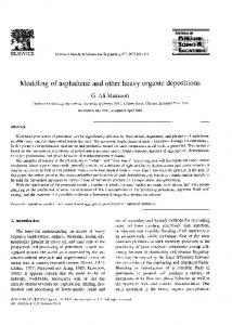
Fig. 1. Prior densities for a single unknown amplitude parameter and the corresponding likelihood functions. The top two distributions depict a prior based on the first ten samples and a likelihood based on the remaining 54 samples. The bottom two distributions show the prior based on the last ten samples and the likelihood based on the first 54 samples. Clearly, the topmost prior is informative for a, while the prior in the third diagram is relatively noninformative for a.

prior density of a is therefore increasingly more informative (smaller 02,) for larger R. Also note that hghR is largest when the samples are taken from the beginning of the time series and smallest when they are taken from the end. For demonstrative purposes, consider the model in (9) with a = 1, f = 0.24, a = 0.05, N = 64, and o2 set to provide a signal-to-noise ratio (SNR)3 of 15 dB. We generated 10000 realizations according to (9) and plotted histograms of &R (this is the empirical density f ( a I XR) based on 10000 trials) for two cases. For the first we constructed f( a I X R ) with the Jirst x[n]= ae-Qn c o s ( 2 r f n ) ~ [ n ] n, = O , l , . , N - 1 (9) R = 10 data samples (which entails that the corresponding likelihLood of a was based on the last 54 observations), where the error sequence E[.] %! N(0,a2).In matrix form, and in the second case we formed f ( a I XR) using the last (9) can be written as R = 10 samples (implying that the likelihood of a was x=ha+e based on the jirst 54 samples). Fig. 1 shows the normalized histograms of i i ~superimposed on the theoretical density where h = [l e-Q c o s ( 2 r f ) e--2Qc o s ( 4 r f ) . e--(N-l)cu f ( u 1 XR), along with the normalized histograms of & N - R cos(2(N - 1)rf)l'. For clarity, take the noise variance a2 superimposed on the theoretical likelihoods ~ ( X N - R I x,a). and the nonlinear parameters f and a to be known constants. The first two distributions are nearly identical, implying that Next we split the data x into XR and X N - R . The prior density approximately the same information is contained in the prior of the parameters in (6) can then be viewed as the posterior as is contained in the likelihood function. That is, f ( a I XR) is of the unknown amplitude a (given the training data XR). The highly informative (relative to its likelihood) when it is based N ( & Rc:~), , and thus quantity (a I XR) on the first R = 10 samples. Conversely, the second pair of histograms demonstrate that f ( a I XR) is locally uniform over -2,: (a-8d2 f(UlXR) e aR the support region of the likelihood function, and thus, it is indeed noninformative relative to the likelihood function. where i c = ~ ( h Z h R ) - ' h g x R and azR = a2(h;hR)-l [2]. It can likewise be shown that decreasing the number of Since the variance a;, is inversely proportional to hghR, samples R decreases the information in the prior, and increasit is clear that increasing hghR causes 02R to decrease. ing 6:increases the information in the prior. Note that this (here, h, is the ith element is consistent with the initial approximation in (5). That is, the Furthermore, hghR = CzEKRh: of h R , and K R c Z, consists of R elements of Z N ) ,so as 31n (this context, SNR refers to the peak S N R that is, the signal-to-noise R increases, h;hR increases, causing a .,; to decrease. The

+

S

.

+

N

ratio of the first sample defined as

*Since the signal is increasingly inundated by noise as the process evolves with time, the last samples of x will contain the least amount of information.

SNR = 10loglo

(

( p

am;1itude)2)

dB.

2c


IEEE TRANSACTIONS ON SIGNAL PROCESSING, VOL. 44, NO. 3, MARCH 1996

614

approximation f(x 1 q ) M ~ contains less information.

I

( X N - R XR,

q ) is better when

XR

111. ORDER SELECTION OF DAMPED SINUSOIDS IN WHITE GAUSSIAN NOISE Consider the data model in (1) wherein the signals s, (n;0,) represent real damped sinusoids and the noise samples ~ [ nN ] N(0,~7'). For this case, the observed data x can be represented by

at the bottom of the page). Here the subscripts N and R in the numerator and denominator indicate that they are based on N , and the last R samples of the data vector x, respectively. Note that the total dimensionality of the integrals is 3q for both numerator and denominator. To lower the total dimension to 2q, we apply the following transformation to the data model in (lo), as follows: 4

i=l

M O: X[n]= € ( n , u 2 ) , 72 E ZN P

M,

:%[.I

=~a,e-""cos(2nf,n

a

+ q%)+

e(n;u2),

i=l

- a, sin q5Ze--cutn sin(a.irf,n)]

2=1

n E

ZN, 4

E { 1 , 2 , . . . , & - 1).

(10)

The unknown parameters associated with the ith signal are its amplitude (a,) , frequency (f,) , phase (4,), and damping factor (a,). The noise power u2 is also assumed unknown. Given the data {z,},~z~, the objective is to estimate the model order q by applying the MAP criterion in (8). Equation (10) can be written concisely in vector-matrix notation as x = A,aq + E ,

where x and t are N x 1 vectors, a, is a q x 1 vector of amplitude constants, and A, is the N x q signal manifold matrix whose ith column is of the €orm a, = [cos(b,)

cos(2nf, + 4,)

x c o s ( 2 n f , ( N - 1)

+ &)IT.

the right-hand side of which can be expressed in matrix form as 4

C[a,cos

cos(2nj,n> - a, sin 4ze--cytnsin(anf,n)l

z=1

=H,b,,

n c ZN

where

(1 1)

q E ZQ

(15)

€3, =

[Cl

SI

b, = [by b:

c2

s2

.. .

cq

%I,

. . . b:lT

with

. . . e--at(N-l)

Since the noise process is white and Gaussian, the likelihood term can be expressed as

To depict a state of ignorance concerning the unknown parameters, we assign the noninformative Jeffreys' prior f(8,, 0 I q ) oc 0-l (see [2]). Combining this and (12), the numerator of (8) can be expressed as

x (xKP&xN)-(w)d4,df,da,,

N > q.

(13)

Applying the transformation in (15) to (10) and following all the steps that led to (14), we arrive at (16), shown at the bottom of the next page. Note that the dimensions of the integrals in (14) have been reduced by a factor of $ as a result of the transformation. Still, their evaluation is not trivial by any means. They will obviously not have a closed-form solution, and we therefore resort to numerical methods. Since the dimension of the parameter space is large,

The matrix Pt) is the projection operator for the left nullspace of A.,,(.), and r(.)is the standard gamma function. The denominator in (8) can likewise be marginalized, the result of which is the following MAP model selection criterion for damped sinusoidal signals in white Gaussian noise (see (14)

a classical technique such as numerical quadrature would be excessively computational. The Monte Carlo method, on the other hand, has long been recognized as a powerful alternative to performing calculations that are considered too complicated for classical techniques.


~

BISHOP AND DJURIC:MODEL ORDER SELECTION OF DAMPED SINUSOIDS IN NOISE

.'

615

IV. MONTECARLOIMPORTANCE SAMPLING INTEGRATION infinite singularities (or near singularities) can be "removed" from the integrand (this is accomplished by sampling from an importance function with a similar singularity in the same location). The fundamental concept behind simple Monte Carlo inteThe asymptotic error variance of an importance sampling gration is to uniformly sample M points {yi}llilM from a estimate strongly depends on the density h(.) (also known multidimensional volume V . Then the Monte Carlo estimate as the importance function) [23]. The three most important of the integral of a function E over V is [18], as follows: properties of a good importance function are as follows. The simplicity by which the random variates yz can be generated from h( .). ' integral estimate h ( . ) should have longer tails than the integrand 128 samples. This result certainly seems more logical. That is, the performance of any statistical criterion should improve to some extent when the phenomenon under study is observed over a longer time interval, and if it does not improve, it certainly should not deteriorate.

+ 1.Oe-O 05n

I n cos(2n(0.2)n)

+

~ 0 ~ ( 2 ~ ( 0 . 2 4 ) hE [)T L ] ,

12

= 0,1, .. . , N

-

1

for sequence lengths of N = 64,100,128,150,200, and 256 samples. Each case consisted of 100 independent trials. For each Of N’ the prediction Order was adjusted so that the backward linear prediction data matrix for the AIC and MDL remained square. This allowed the AIC and MDL to perfom optimally [211. The results of this experiment are shown in Table 11. Clearly, the performance of the AIC and MDL deteriorated as the number of data samples exceeded the informationbearing portion of the observation vector. Conversely, the performance o f the MAP criterion improved with more data.

For when 64 the MDL and MAP performed almost identically, but as N increased to 128

In this paper, following the Bayesian approach to model selection, we investigated a MAP criterion for selecting the model order of superimposed signals in noise. The criterion was applied to the case of damped sinusoidal signals in i.i.d. white Gaussian noise, and its performance was compared to the SVD-based AIC and MDL. Our criterion proved to be more consistentthan either of the others for damped sinusoidal data models. Computer simulations provided for a comparison between the MAP, AIC, and MDL criteria. REFERENCES [ 13 H. Akake, “A new look at statistical model identification,”IEEE Trans

Automat Contr , vol AC-19, pp 716-723, Dec 1974 [23 G. E Box and G C Tiao, Bayesian Inference in Statistical Analysis Reading, MA. Addison-Wesley, 1973 [3] R N Bracewell, ‘‘Rad0 interferometry of discrete sources,” Proc IRE, V O ~46, pp 97-105 1958 [4] Y Bresler and A Macovslu, “Exact maximum likelihood parameter estimation of supenmposed exponentd signals in noise,” IEEE Trans Acoust , Speech, Signal Processing, vol ASSP-34, no 5, 1986 I51 P. J. Davis and P Rabinowitz. Methods ofNumerical Intearation New York Acadenxc, 1975 [6] P. M Djun6, “Selection of signal and system models by Bayesian predictive densities,” Ph D dissertation, Univ. of Rhode Island, Kmgston, 1990 [7] P M Djun6 and S M Kay, “Order selection of autoregressivemodels,” IEEE Tram Srgnal Processmg, vo1 40, no 11, pp 2829-2833, 1992 [SI -, “Model selection based on Bayesian predictive densitm and multiple data records,” IEEE Trans Signal Processing, vol 42, no 7, pp 1685-1699, 1994 [9] P. M. Djurie, “Model selection based on asymptotic Bayes theory,” In Proc. 7th SP Workshop Statist. Signal Array Processing, P Q , Canada, 1994, pp 7-10. [lo] C G M. Fant, Acoustic Theory of Speech Production The Hague, The Netherlands. Mouton, 1960. [11] M Feder and E Welnsteln, “parmeter eStlmabOn of superimposed signals using the EM algonthm,” IEEE Trans Acoust , Speech, Signal Processing, vol 36, pp 477489, 1988 [121 N. Floumey and R. K. Tsutakawa, Eds , Statistical Multiple Integration. American Mathematical Society Series in Contemporary Mathematics,vol 115. 1989. [13] S Geisser, “Aspects of the predictive and estimative approaches in the determmahon of probabilities,” Biometrics (supplement), vol 38, pp 75-85, 1982. [14] J Geweke, Bayesian Inference in Econometric Models Using Monte Carlo Integration. Durham, NC Dept of Econometrics, Duke University, 1986. [15] P Horst, Prediction ofPersonalAdjustment. New York Social Science Research Council, Bulletin 48, 1941.


BISHOP AND DJURIC: MODEL ORDER SELECTION OF DAMPED SINUSOIDS IN NOISE

[I63 C. M. Hurvich and C. L. Tsai, “A corrected Akaike information criterion for vector autoregressivemodel selection,” J. Time Series Anal., vol. 14, no. 3, pp. 271-279, 1993. F. James, “Monte Carlo theory and practice,” Reports on Progress in Physics, vol. 43, pp. 1145-1175, 1980. M. H. Kalos and P. H. Whitlock, Monte Carlo Methods. New York: Wiley, 1986. L. Kavalieris and E. J. Hannan, “Determining the number of terms in a trigonometric regression,” L Time Series Anal., vol. 15, no. 6, pp. 613-625, 1994. K. Kloek and H. K. van Dijk, “Bayesian estimates of equation system parameters: An application of integration by Monte Carlo,” Econometrica, vol. 46, pp. 1-20, 1978. R. Kumaresan and D. W. Tufts, “Estimating the parameters of exponentially damped sinusoidal signals and pole-zero modeling in noise,” IEEE Trans. Acoust., Speech, Signal Processing, vol. 30, no. 6, pp. 833-840, 1982. P. W. Laud and J. G. Ibrahim,”Predictive model selection,” J. Royal Statist. Soc. B , vol. 57, no. 1, pp. 247-262, 1995. M . 3 . Oh, “Monte Carlo integration via importance sampling: dimensionality effect and an adaptive algorithm,” in Multiple Statistical Integration, vol. 115. American Mathematical Society, 1989. F. Mosteller and D. L. Wallace, “Inference in an authorship problem,” J. Amer. Statist. Assoc., vol. 58, pp. 275-309, 1963. J. Myhill et al., “Investigation of an operator method in the analysis of biological tracer data,” Biophysical J., vol. 5, pp. 89-107, 1965. A. O’Hagan, “Fractional Bayes factors for model comparison,” J. Royal Statist. Soc. B, vol. 57, no. 1, pp. 99-138, 1995. M. H. Quenoille, “Notes on bias in estimation,” Biometrika, vol. 42, pp. 353-360, 1956. V. U. Reddy and L. S. Biradar, “SVD-based information theoretic criteria for detection of the number of dampedundamped sinusoids and their performance analysis,” IEEE Trans. Signal Processing, vol. 41, no. 9, pp. 2872-2881, 1993. J. Rissanen, “Modeling by shortest data description,” Automatica, vol. 14, pp. 465-471, 1978. -, “A predictive least-squares principle,” IMA J. Math. Contr. Inform., vol. 3, pp. 211-222, 1986. -, “Stochastic complexity,” J. Royal Statist. Soc., Series B, Methodol., vol. 49, no. 3, pp. 240-265, 1987. -, “Stochastic complexity in scientific inquiry,” in World Scientijic Series in Computer Science, vol. 15, 1989. H. V. Roberts, “Probabilistic prediction,” J. Amer. Statist. Assoc., vol. 60, pp. 50-62, 1965. R. Y. Rubinstein, Simulation and the Monte Carlo Method. New York: Wiley, 1981. G . Schwartz, “Estimating the dimension of a model,” Annals Statist., vol. 6, no. 2, pp. 461464, 1978. L. Stewart, “Bayesian analysis using Monte Carlo integration-A powerful methodology for handling some difficult problems,” Statistician, vol. 32, pp. 195-200, 1983. I

619

1371 . . M. Stone, “Cross-validatory choice and assessment of statistical uredictions,” J. Royal Statist. SoE. B, vol. 41, pp. 111-147, 1974. [38] S. Umesh and D. W. Tufts, “Estimation of parameters of many exponentially damped sinusoids using fast maximum likelihood estimation wiith application to NMR spectroscopy data,” submitted to IEEE Trans. Signal Processing. [39] C. S. Wallace and D. M. Boulton, “An information measure for classification,” Computer J., vol. 11, no. 2, pp. 185-194, 1968. [40] C. S. Wallace and P. R. Freeman, “Estimation and inference by compact coding,” J. Royal Statist. Soc., Series B, Methodol., vol. 49, no. 3, pp. 2410-265, 1987. [41] M. Wax and T. Kailath, “Detection of signals by information theoretic criteria,” IEEE Trans. Acoust., Speech, Signal Processing, vol. ASSP-33, no. 2, 1985. ~

William B. Bishop (S’94) was born in Long Island, New York. He received the B.E. and M.S. degrees from the State University of New York (SUNY) at Stony Brook, NY, USA, in 1990 and 1991, respectively. From 1992 to present he has been with the Department of Electrical Engineering, SUNY, as both a research assistant and teaching assistant, and is currently a candidate for the Ph.D. degree. His research interests are in the areas of statistical signal modeling and estimation theory. Mr. Bishop is a member of the American Statistical Association.

Petar M[.DjuriC (S’86-M’90) was born in Strumica, Yugoslavia. He received the B.S. and M.S. degrees from the University of Belgrade, Yugoslavia, in 1981 and 1986, respectively,, and the Ph.D. degree from the University of Rhode Island, Providence, RI, USA, in 1990, all in electrical engineering. From 1981 to 1986, he was with the Institute of Nuclear Sciences-Vinca, Computer Systems Design Department, where he conducted research in digital and statistical signal processing, communications, and pattern recognition. From 1986 to 1990, he was a research and teaching assistant in the Department of Electrical Engineering at the University of Rhode Island. He joined the Department of Electrical Engineering at the State University of New York at Stony Brook, NY, USA, in 1990, where he is currently an assistant professor. His main research interests are in statistical signal processing and signal modeling. Dr. DjuriC is a member the American Statistical Association. Currently, he ON SIGNAL PROCESSING. serves as an associate editor for IEEE TRANSACTIONS
