Model selection and Bayesian inference for high-resolution seabed ...

Model selection and Bayesian inference for high-resolution seabed reflection inversion Jan Dettmera兲 and Stan E. Dosso School of Earth and Ocean Sciences, University of Victoria, Victoria BC V8W 3P6, Canada

Charles W. Holland Applied Research Laboratory, State College, The Pennsylvania State University, State College, Pennsylvania 16804-0030

共Received 6 August 2008; revised 26 November 2008; accepted 3 December 2008兲 This paper applies Bayesian inference, including model selection and posterior parameter inference, to inversion of seabed reflection data to resolve sediment structure at a spatial scale below the pulse length of the acoustic source. A practical approach to model selection is used, employing the Bayesian information criterion to decide on the number of sediment layers needed to sufficiently fit the data while satisfying parsimony to avoid overparametrization. Posterior parameter inference is carried out using an efficient Metropolis–Hastings algorithm for high-dimensional models, and results are presented as marginal-probability depth distributions for sound velocity, density, and attenuation. The approach is applied to plane-wave reflection-coefficient inversion of single-bounce data collected on the Malta Plateau, Mediterranean Sea, which indicate complex fine structure close to the water-sediment interface. This fine structure is resolved in the geoacoustic inversion results in terms of four layers within the upper meter of sediments. The inversion results are in good agreement with parameter estimates from a gravity core taken at the experiment site. © 2009 Acoustical Society of America. 关DOI: 10.1121/1.3056553兴 PACS number共s兲: 43.30.Pc, 43.30.Ma, 43.60.Pt 关AIT兴

I. INTRODUCTION

Knowledge of seabed sediment geoacoustic properties is important for a variety of acoustic/sonar applications in shallow water environments, and inferring information about sediment properties from acoustic data has received wide attention.1–16 In recent years, Bayesian inference has been applied increasingly to yield optimal parameter estimates and quantify parameter uncertainties and interrelationships using Markov chain Monte Carlo 共MCMC兲 methods to estimate the posterior probability density 共PPD兲.8–16 This paper considers Bayesian inference for high-resolution seabed reflection-coefficient data to infer fine-scale local sediment structure with the ultimate goal of quantifying spatial variability in sediments. The data are obtained using an experimental procedure developed by Holland and Osler6 using a bottom-moored hydrophone and a ship-towed impulsive source 共e.g., seismic boomer兲. Due to the local scale 共⬃100 m seabed footprint兲, the effects of spatial and temporal variabilities in the water column and seabed are greatly reduced compared to long-range acoustic measurements. Further, impulsive sources with a large bandwidth to high frequencies have potential to resolve fine structure in the uppermost sediment. The inversion is carried out using a plane-wave reflection-coefficient forward model.10 Seismoacoustic reflection data can be inverted in the time and/or frequency domains to yield seabed soundvelocity, density, and attenuation profiles.9–11 Dettmer et al.11 selected the model parametrization by estimating the number

a兲

Electronic mail: [email protected]

706

J. Acoust. Soc. Am. 125 共2兲, February 2009

Pages: 706–716

of sediment layers as the number of distinct reflected arrivals in a sequential Bayesian inversion of time- and frequencydomain data. However, high-quality single-bounce reflection-coefficient data can contain information about sediment layers with thicknesses much less than the typical boomer pulse length 共⬃0.5 m at 1500 m / s兲 in the experiment. In particular, high-quality broadband data that extend to high frequencies 共several kilohertz兲 can contain information about layers of order of centimeters. In such cases, timedomain data are not sufficient to address model selection 共e.g., model parametrization兲 because distinct reflected arrivals for each layer cannot be identified. Model selection is a common aspect of geoscientific inverse problems, where complex unknown environments often result in nonuniqueness and unknown theory error. A model is considered to be any particular choice of physical theory, its appropriate parametrization, and a statistical representation for the data errors that are used to explain the observed physical system. The goal of the selection is to determine the simplest model that sufficiently explains the data by applying a parsimony criterion. In this paper, parametrization of the model is considered in terms of the number of layers. Model comparison is also a central problem for studying spatial sediment variability. Meaningful comparison of sediment structure between sites requires a scheme to quantify uncertainty at each site, including uncertainty due to the model parametrization selected. Model selection is particularly important for high-quality data, since poor model selection will result in systematic errors, potentially causing biased results. It is important to note that while underparametrizing a model can be desirable in terms of simplicity, it

0001-4966/2009/125共2兲/706/11/$25.00

© 2009 Acoustical Society of America

can also lead to unrealistically small parameter uncertainty estimates and large theory error. A simple model will reach high likelihood levels only for specific parameter values; it can only access a limited part of the data space and therefore will indicate small uncertainties for the predicted parameters, which can be misleading. Furthermore, the theory error introduced by underparametrization can lead to biases in the parameter estimates. Hence, it is important to select an appropriate parametrization based on an objective criterion. Which and how many models are considered in a study depend largely on subjective choices such as the intended use of the model and prior knowledge of the environment. Several approaches exist to examine models by quantifying their likelihood using point estimates 关e.g., evaluated at the maximum a posteriori 共MAP兲 model vector兴.17,18 For example, assuming Gaussian-distributed data errors, ␹2 probabilities can be used to evaluate the likelihood of a model at single points in the model spaces considered. An F-test can be used to calculate the allowable change in the ␹2 misfit for given levels of significance.19 The main problem with the maximum-likelihood method is that it is biased toward unjustifiably complex models,18 which is in conflict with the generally accepted concept of Ockham’s razor20,21 that empirically demands preference of simple models. To avoid this bias, asymptotic methods such as the Akaike information criterion 共AIC兲共Ref. 22兲 have been introduced. However, the AIC is still biased toward complex models for large data sets.23 The Bayesian information criterion 共BIC兲23,24 is related to Bayesian factors and eliminates the bias by accounting for the number of data. The BIC is used for model selection in this paper. The class of models considered here are multilayered sediment models defined by layer thickness, sound velocity, density, and attenuation, and the model selection problem is to determine the optimum number of sediment layers required to sufficiently match the observed data while satisfying parsimony. High-dimensional model spaces 共up to 35 parameters兲 and strong parameter correlations are addressed by an efficient MCMC sampling scheme using the Metropolis–Hastings 共MH兲 algorithm in principalcomponent space with a Cauchy proposal distribution.25 The scaling of the Cauchy distribution is initially based on a linear approximation of the PPD around a likely model, and progressively transformed into a nonlinear estimate during the burn-in phase.25 A massively parallel algorithm implementation is developed to allow feasible application to complicated and computationally demanding problems.10 To summarize, this paper illustrates how layered profiles can be resolved from seabed reflection data collected with an acoustic-source pulse length that is large compared to the layering structure. The inherent nonuniqueness of the problem is practicably addressed by applying the BIC to ensure parsimony of inversion results. The remainder of the paper is structured as follows. In Sec. II, Bayesian inference is reviewed with an emphasis on model comparison. The Bayesian inference is then applied to data collected on the Malta Plateau, Mediterranean Sea, in Sec. III. In Sec. III C the model selection is carried out applying the BIC to the MAP model parameters from the inJ. Acoust. Soc. Am., Vol. 125, No. 2, February 2009

version. Finally, Sec. III D presents the results in terms of geoacoustic profiles for the selected model, and compares the results to cores taken at the experiment site. II. BAYESIAN INFERENCE

This section gives a brief overview of the Bayesian formulation of inverse problems; more complete treatments can be found elsewhere.21,26–30 Let d 苸 RN be a random variable of N observed data containing information about a physical system. Further, let I denote the model specifying a particular choice of physical theory, model parametrization, and error statistics to explain that physical system. Let m 苸 R M be a random variable with M free parameters representing one realization of the model I. Bayes’ rule can then be written as P共m兩d,I兲 =

P共d兩m,I兲P共m兩I兲 P共d兩I兲

共1兲

,

where the conditional probability P共m 兩 d , I兲 represents the PPD of the unknown model parameters given the observed data, prior information, and choice of model I. The conditional probability P共d 兩 m , I兲 describes the data-error statistics. Since data errors include measurement and theory errors 共which cannot generally be separated兲, the specific form of this distribution is often not known. To interpret Eq. 共1兲 quantitatively, some particular form that describes the dataerror statistics reasonably well must be assumed for this distribution. In practice, mathematically simple distributions, such as multivariate Gaussian distributions, are commonly used; the validity of such assumptions should be checked using statistical tests.11,12 共Other distributions can be used as long as an appropriate likelihood function can be formulated; e.g., double exponential distributions are commonly applied for data sets that include large outliers.30兲 The general multivariate Gaussian distribution for real data is given by P共d兩m,I兲 =

1 共2␲兲兩Cd兩1/2 N/2

冉

冊

1 ⫻exp − 共d − d共m兲兲TC−1 d 共d − d共m兲兲 , 共2兲 2 where Cd is the data covariance matrix and d共m兲 is the modeled data. The covariance matrix Cd is often unknown since the source of errors may be poorly understood. In some cases, data-error statistics can be parametrized 共e.g., as variances or as a covariance matrix based on an assumed form such as an autoregressive moving average19兲 and included in the inversion, either implicitly31 or explicitly as unknown hyperparameters with assigned priors.31–33 Data-error covariance matrices can also be estimated nonparametrically from data residuals 共i.e., the difference between modeled and measured data, considered later兲. In inverse theory, P共d 兩 m , I兲 is interpreted as a likelihood function L共m 兩 I兲 of m for fixed 共observed兲 data d. Note that given a Gaussian data-error distribution, the likelihood function is not Gaussian distributed for nonlinear inverse problems. The term P共m 兩 I兲 in Eq. 共1兲 gives the model prior distribution. In this paper, prior distributions are considered to be bounded, uniform distributions of the form Dettmer et al.: Model selection and Bayesian inference

707

P共m兩I兲

=

冦

M共I兲

共m+i − m−i 兲−1 兿 i=1

if m−i ⱕ mi ⱕ m+i , i = 1,M共I兲

0

else.

冧

共3兲

The conditional probability P共d 兩 I兲 is commonly referred to as the evidence or marginal likelihood of I. It describes how likely a certain parametrization I is given the observed data and prior. Since the evidence P共d 兩 I兲 normalizes Eq. 共1兲, it can be written as Z共I兲 = P共d兩I兲 =

冕

P共d兩m,I兲P共m兩I兲dm.

M

共4兲

A. Estimating the PPD

To estimate the PPD for a fixed choice of model I, MCMC sampling methods are usually applied.21,28,29,34,35 The PPD can then be used to obtain model parameter and uncertainty estimates. For a fixed parametrization, Eq. 共1兲 can be written as P共m兩d,I兲 ⬀ L共m兩I兲P共m兩I兲,

共5兲

where P共m 兩 d , I兲 quantifies the state of information about the model parameters given the data, prior information, and parametrization. This paper considers the likelihood function to be of the form given by Eq. 共2兲. For inference it is common to work with the log-likelihood to avoid floating-point underflow due to the exponential dependence. The multidimensional PPD is generally interpreted in terms of properties ˆ , the a posteriori such as the MAP model vector estimate m ¯ , the model covariance matrix Cm, and mean model vector m marginal-probability distributions P共mi 兩 d兲, defined as ˆ = argmax P共m兩d,I兲, m ¯ = m

冕

M

Cm =

m⬘ P共m⬘兩d,I兲dm⬘ ,

冕

M

P共mi兩d兲 =

共6兲共7兲

¯ 兲共m⬘ − m ¯ 兲T P共m⬘兩d,I兲dm⬘ , 共m⬘ − m

共8兲

冕

共9兲

M

␦共mi⬘ − mi兲P共m⬘兩d,I兲dm⬘ ,

where ␦ denotes the Dirac delta function. Higherdimensional marginal distributions can be defined similar to Eq. 共9兲. While analytic solutions to Eqs. 共6兲–共9兲 exist for linear inverse problems, nonlinear problems such as geoacoustic inversion must be solved numerically. MAP estimates 关Eq. 共6兲兴 can be found by numerical optimization methods, such as adaptive simplex simulated annealing 共ASSA兲, which combines the local downhill simplex method within a very fast simulated annealing global search.5 For the inversion considered in this paper, the optimization problem is particularly challenging with large num708

J. Acoust. Soc. Am., Vol. 125, No. 2, February 2009

bers of parameters, and a parallel implementation of the ASSA optimization was developed employing message passing.36 Parallel ASSA uses as many simplexes as the number of available central processing units 共CPUs兲. On each CPU, a single simplex is optimized for a certain number of steps using the usual scheme.5 The models of all simplexes are then randomly regrouped into new simplexes and ASSA optimization is again performed for a certain number of steps before the regrouping process is carried out again, and so on until convergence. This optimization searches the parameter space more thoroughly than an algorithm with one simplex, and makes optimization of complicated problems feasible. Detailed performance studies to examine the scaling of the parallel ASSA algorithm with the number of CPUs were not carried out. The integrals of Eqs. 共8兲 and 共9兲 are computed here using MCMC sampling that applies an adaptive MH algorithm.34,35 The implementation follows Dosso and Wilmut.25 Initially, the algorithm computes a linearized PPD approximation around a reasonably good starting model. This yields an approximate linear model covariance matrix that can be used for a principal-component rotation of the parameter space where the coordinate axes align with the dominant correlation directions around the starting model. During a burn-in phase, the linear model covariance matrix is progressively replaced with a fully nonlinear covariance estimate. To further ensure efficient sampling of the posterior, perturbations in the Markov chain are drawn from a Cauchy proposal distribution that is scaled by the eigenvalues of the covariance matrix, which represent variances of the principal components. During sampling, chain thinning26 is applied to keep reasonably small sample sizes for models with large numbers of parameters. The algorithm is massively parallel for feasibility.11 B. Model selection

Bayesian evidence 共also referred to as the normalizing constant or free energy兲, Eq. 共4兲, and Bayesian factors 共the ratio of evidences for two models兲 are the basis for model selection. Evidence brings a natural parsimony to the model selection problem, which is also referred to as the Bayesian razor. In contrast to Ockham’s razor, Bayesian model selection is not based on a qualitative preference for model parsimony based on aesthetic or empirical reasons, but rather favors parsimony intrinsically and quantitatively.21 Estimating evidence is challenging due to the requirement to integrate the likelihood with respect to the prior,37 and finding robust and accurate estimators for the evidence integral has seen the attention of much research. Note that evidence estimates should ideally be future proof, allowing future researchers to compare results obtained for the same data by different techniques.38 Several methods to approximate evidence by predictive distributions and by analytical examination of asymptotic behavior can be found in literature.17,18 Further, numerous attempts in the statistics community have been made to find MCMC sampling estimators that are based on the posterior.18,37,39–41 Several estimators 共dependent on the inDettmer et al.: Model selection and Bayesian inference

BIC共I兲 = − 2 loge L共mML兩I兲 + M loge N.

共10兲

Since the BIC is based on the negative log likelihood, the model with the smallest BIC is selected as the preferred model. The value of the BIC cannot be directly associated with a probability and cannot yield the significance of the selection. In comparison to the also commonly used AIC,22 AIC共I兲 = − 2 loge L共mML兩I兲 + 2M ,

0

50 Depth (m)

verse likelihood兲 have been shown to be unstable.37 Others, such as importance sampling based on the posterior,18 have been applied40 including an application to geoacoustic inversion.15 However, significant problems exist with this approach since evidence depends on the likelihood’s relationship to the prior.42,43 This can lead to unstable and inaccurate results due to only sampling from the posterior. Results are also sensitive to the choice of importance sampling function.28,37,42,43 Evidence can also be addressed by treating the inversion as a transdimensional problem and applying reversible-jump Markov chains44 that can jump between spaces of different dimensionalities. Although interesting for future applications, transdimensional inversion is challenging and implementation for general problems is difficult.34,45 Reversiblejump Markov chains also require specifying all models to be considered a priori. Other Monte Carlo based methods that also/only sample from the prior such as thermodynamic integration,40,46 annealed importance sampling,47 and nested sampling38 exist that can give unbiased estimates of the evidence for general problems. However, the associated computational cost of these methods is high. Due to the high computational demands of the forward and inverse problems considered in this paper, an asymptotic point estimate 共for the maximum-likelihood model vector mML兲 is used to carry out model selection. The BIC23,24 is an asymptotic approximation derived for diffuse multivariate normal prior distributions 共with mean at the maximumlikelihood estimate and variance of the Kullback–Leibler expected information兲.48 The BIC is given by

100

150 1511

1515

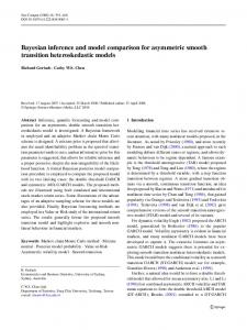
FIG. 1. Original conductivity temperature depth profile 共solid line兲 and approximated sound-velocity profile 共dashed line, used for the inversion兲 collected at site 13 on the Malta Plateau.

water depth was 144 m. The sound-velocity profile is shown in Fig. 1 and was fairly constant with the sound velocity varying less than 5 m / s over the water column. The source was towed at 0.3 m depth. Figure 2 shows part of the seismoacoustic traces 共in reduced time兲 with the lines across traces indicating the direct arrival and the part of the bottom response used to compute the reflection coefficients. Figure 2 also illustrates the need for an objective model selection criterion. Reflected energy is most concentrated around the water-sediment interface reflection at 0.109 s and at a later event at about 0.114 s 共times are given here for the shortest-range trace兲. In both instances, the events are spread out in time and the model parametriza-

共11兲

the BIC corrects for the number of data and favors simpler models than the AIC for N ⬎ 8. The AIC has been shown to yield excessively complex models, particularly for large numbers of data.23 Since this study addresses large data sets, the BIC is used here for model selection.

A. Experiment and data

This section applies the inversion and model selection to seismoacoustic reflection data collected April 6, 2002, during the Boundary02 experiment at 36° 24.515⬘ N, 14° 38.142⬘ E on the Malta Plateau, Mediterranean Sea. The acoustic data were generated with an electromechanical impulsive source 共GeoAcoustics 5813B Geopulse boomer兲 with a short pulse length 共⬍1 ms兲 and a broad bandwidth 共0.5– 10 kHz兲. Data were recorded at a single receiver that was part of a vertical line array of four hydrophones, and sampled at 48 kHz. The hydrophone used in this data set was at 124 m depth and the

0.08

0.085

0.09

Reduced Time (s)

III. INVERSION RESULTS


1512 1513 1514 Sound Speed (m/s)

0.095

0.1

0.105

0.11

0.115

0.12 100

200

300

400 Range (m)

500

600

700

FIG. 2. Seismoacoustic traces 共in reduced time, with 1512 m / s reducing velocity兲 collected at site 13 on the Malta Plateau. Dettmer et al.: Model selection and Bayesian inference

709

Refl. Coeff.

0.9

1000 Hz

1200 Hz

1400 Hz

1683 Hz

1889 Hz

2121 Hz

2381 Hz

2672 Hz

3000 Hz

3367 Hz

3779 Hz

4242 Hz

30 60 4762 Hz Angle (deg.)

30 60 5345 Hz Angle (deg.)

30 60 Angle (deg.)

30 60 Angle (deg.)

0.6 0.3 0

Refl. Coeff.

0.9 0.6 0.3 0 Refl. Coeff.

0.9

30 60 Angle (deg.)

0.6 0.3 0

30 60 Angle (deg.)

30 60 Angle (deg.)

FIG. 3. Reflection-coefficient data as a function of grazing angle and frequency 共band centers indicated兲. The solid line indicates the best fit obtained from the MAP parameters of the model selected by the BIC 共five layers兲.

Frequency (Hz)

tion is not obvious: Both zones could contain reflections from one or more layers as individual reflectors cannot be clearly identified. Reflection-coefficient data as a function of grazing angle and frequency were computed from time-windowed direct and bottom-reflected arrivals using the method of Holland,7 and are shown in Fig. 3. In this case, the bottom response is time windowed to approximately 6 m depth below the seafloor for ranges between 25 and 740 m, as indicated in Fig. 2. The data are averaged into 14 frequency bands from 1000 to 5300 Hz using a Gaussian frequency average10,49 with a fractional bandwidth of 1 / 10 of the center frequency, resulting in bandwidths from 100 to 530 Hz. Figure 4 shows reflection-coefficient data that are averaged over 5 Hz bands and compares these to the reflection-coefficient data that are used in the inversion. The fractional bandwidth of 1 / 10 was

found to retain structure in the reflection-coefficient data while reducing noise and resulting in reflection-coefficient data that are computationally feasible in the inversion. The data are interpolated onto a uniform spacing in angle; points with a signal to noise ratio of less than 6 dB were excluded. Further, interpolated data that fall into recording gaps 共due to experiment design兲 are excluded from the inversion. This results in approximately 90 data at each frequency with an angular range from 12° to 81°. B. Forward model

The forward model consists of a plane-wave reflectioncoefficient model that approximates the seabed as a layered lossy fluid.11 The replica reflection-coefficient data for each frequency band are computed using the same frequency av-

5000

5000

4500

4500

4000

4000

3500

3500

3000

3000

2500

2500

2000

2000

1500

1500

1000

20

30

40 50 Angle (deg.)

60

70

80

1000

20

30

40 50 Angle (deg.)

60

70

80

FIG. 4. 共Color online兲 Reflection-coefficient data 共clipped at 1.0兲 as a function of grazing angle and frequency. The left panel shows reflection-coefficient data for a narrow, constant 5 Hz band average and the right panel shows the data used in the inversion, averaged with a fractional bandwidth of 1 / 10. 710


Dettmer et al.: Model selection and Bayesian inference

eraging as used for the measured data. However, to address limited computational time, the number of frequencies in the average is limited to 12 frequencies per band. A forward modeling study was carried out to ensure that full-wave field effects are negligible and that plane-wave modeling is sufficient.10

BIC

2

10

0

AIC

10

2

10

2.9

The model selection study was carried out using two groups of models. Group A assumes an increasing number of layers for the uppermost part of the sediment 共corresponding to the reflected arrivals beginning at 0.109 s in Fig. 2兲 and a single reflector at depth 共corresponding to the deeper reflected arrivals at 0.114 s兲. Group B considers the same numbers of layers for the uppermost part of the sediment but contains two reflectors 共i.e., a layer兲 at depth. This way both zones that show reflections in the time series are addressed by the model selection. Group A includes five models with three to seven layers and group B includes seven models with two to eight layers. For each model the total number of parameters in the inversion increases by 4 with each additional layer. To obtain inversion and model selection results, dataerror statistics were estimated from the reflection-coefficient processing7 and optimization was carried out using planewave reflection-coefficient inversion.12,14 Prior bounds were chosen to be uniform over wide intervals. However, the thin topmost layers were differentiated by choosing prior bounds for layer thickness from 5 to 50 cm. This seems justified since the uppermost events in the time series 共Fig. 2兲 extend over about 1.5 m 共at 1500 m / s兲. These priors also allow the more complex models to exactly represent the simpler models. The resulting likelihood values were used to calculate the BIC for all models and results are shown in Fig. 5. All values are plotted on a loge scale since the range of values is large 共due to the fact that the two-and three-layer models are very

min(-log(L))

C. Model selection

10

2.6

10

2

3

4

5 No. Layers

6

7

8

FIG. 5. BIC, AIC, and negative log likelihood for group A 共open circles兲 and group B 共asterisks兲 on a loge scale. Note that for presentation purposes BIC and AIC values have been shifted so that the minimum value of each is unity.

unlikely with high BIC and AIC values兲. This figure shows that, based on the minimum value of the BIC, the five-layer model from group A is selected. The BIC values for the models in group B do not reach values as low as those for group A, but consistently decrease with more complex parametrizations. This result indicates that the data show high sensitivity to the presence of several layers close to the sediment-water interface. In addition, the simpler models of group A are preferred over the models of group B which contain more structure at depth. Figure 5 also shows the negative log likelihood 共i.e., the data misfit兲 for all parametrizations. It is important to note that these values consistently decrease with an increasing number of layers. The BIC depends strongly on the likelihood values, and a better fit to the data for more complex models is important for the BIC to yield meaningful results. For comparison, the figure also shows the AIC values, with the minimum for both groups occurring at the models with most layers. This bias toward too-complex models for large data sets is commonly observed in other problems.23

1 2 3 Layer thickness (m)

1500 1600 1700 Velocity (m/s)

1.4

1.6 1.8 2 Density (g/cm3 )

0

0.5 Attenuation (dB/λ)

1

FIG. 6. Marginal-probability distributions for the five-layer model from group A. Note that for presentation purposes all marginals are scaled to the same height, not to unit area. Units for attenuation are given in terms of decibels per wavelength 共␭兲. J. Acoust. Soc. Am., Vol. 125, No. 2, February 2009


711

0

1

Depth (m)

2

3

4

5 1500

1600 1700 Velocity (m/s)

1.4 1.6 1.8 Density (g/cm3)

2

0


1

FIG. 7. 共Color online兲 Marginal-probability depth distributions and MAP sediment profiles 共solid line兲 for the five-layer model of group A 共selected by BIC兲. A core 共solid line with error bars兲 taken on site is shown for comparison, with error bars shown for every fifth datum. The left panel also shows the acoustic-source pulse 共at 1500 m / s兲.

D. Posterior parameter inference

Once the preferred model parametrization was identified using the BIC, the data residuals for this model were used to compute a nonparametric estimate of the data-error covariance matrix at each frequency.11 Posterior statistical tests ˆ 兲 and for standardwere carried out for raw residuals d-d共m ˆ 关d-d共m 兲兴 to ensure that these estimates ized residuals C−1/2 d and the assumptions of random Gaussian errors were reasonable. The run test for randomness failed at all 14 frequencies 共at the 0.05 level兲 for raw residuals; however, standardized residuals passed the test at 13 out of 14 frequencies. The Kolmogorov–Smirnov test for Gaussianity was passed 共at the 0.05 level兲 four times for the raw residuals and nine times for the standardized residuals. Overall, the results of the statistical tests suggest the data-error statistics are reasonably well quantified, providing confidence in the inversion results. The estimated error covariance matrices were then used in the integration of the PPD by MH sampling. The integration was carried out for three models from group A, the five-layer model that was picked due to the BIC and the models with three and seven layers to observe the variability in results with model selection. The fit to the measured data for the five-layer model is shown in Fig. 3, and marginal distributions are shown in Fig. 6. The marginal distributions indicate generally well-resolved parameters with distinct changes in sound velocity and density between layers. Attenuation shows low resolution in thin layers but high resolution within the fourth layer of about 4 m thickness. Figure 7 shows the MAP sediment profiles and associated uncertainties in terms of marginal-probability depth distributions for the five-layer model. The uncertainties are obtained from a large random subset of the PPD 共4 ⫻ 105 712


models兲. The inversion results indicate four layers within the upper meter of the sediments. Figure 7 also shows the acoustic-source pulse 共at 1500 m / s兲 for comparison with the inversion results: Note that the pulse length is large compared to the layered structure resolved in the upper sediments. The appearance and location of the thick layer are consistent with what would be expected from the timedomain data 共Fig. 2兲 where no significant reflections occur between 0.11 and 0.113 s. The inversion result also shows an interface at about 4.5 m depth. Confidence for the half-space parameter values, particularly density, is low, likely because the half-space lacks a lower reflector and hence data information is available only from the reflection off the upper interface. Figure 7 also shows the sound-velocity and density estimates from a shallow gravity core taken at the site. The core error bars, shown for every fifth datum, represent measurement errors associated with the time-of-flight and gamma-ray attenuation density estimates for a perfectly calibrated system, but do not include errors due to sediment disturbance from sampling, retrieval, and storage. Note that the core represents a highly localized sample 共10 cm diameter compared to the ⬃100 m experiment footprint兲 and that spikes in the core values could be due to anomalies such as seashells. The core indicates a complicated structure in the upper part of the sediment. The inversion results show a similar fine structure to the core. In particular, the density profile estimate from the inversion matches the core profile estimate well: The location of interfaces in the inversion result coincides with interfaces in the core. Below about 0.5 m depth, the inversion results appear to represent an average value in the sound velocity estimated by the core. Dettmer et al.: Model selection and Bayesian inference

Refl. Coeff.

0.9

1000 Hz

1200 Hz

1400 Hz

1683 Hz

1889 Hz

2121 Hz

2381 Hz

2672 Hz

3000 Hz

3367 Hz

3779 Hz

4242 Hz

30 60 4762 Hz Angle (deg.)

30 60 5345 Hz Angle (deg.)

30 60 Angle (deg.)

30 60 Angle (deg.)

0.6 0.3 0

Refl. Coeff.

0.9 0.6 0.3 0 Refl. Coeff.

0.9

30 60 Angle (deg.)

0.6 0.3 0

30 60 Angle (deg.)

30 60 Angle (deg.)

FIG. 8. The best fit obtained from the MAP parameters of the three-layer model of group A.

Figures 8 and 9 show inversion results for the threelayer model from group A. The fit to the data 共Fig. 8兲 is considerably worse than that for the five-layer model 共Fig. 3兲, and the resulting low log-likelihood value dominates the BIC, resulting in the rejection of the three-layer model. However, high frequencies show a much better fit than low frequencies, suggesting that the model is more appropriate for the shallowest structure than for the deep structure. This is also evident in the marginal distributions in Fig. 9, which show that the first layer of about 10 cm thickness is resolved. However, the sound velocity for the uppermost layer is likely biased and appears high compared to the water sound veloc-

ity of 1513 m / s 共see Fig. 1兲. The reason for this effect in sound velocity is likely the underparametrization of the three-layer model, which causes the surficial layer to account for not only the uppermost sound velocity but also somewhat the deeper sound-velocity structure. Below that, the soundvelocity results seem to approximately average over the core structure shown in Fig. 7 in a similar fashion. The density inversion results appear to be consistently too low compared to the five-layer model and the core. Figures 10 and 11 show inversion results for the sevenlayer model from group A. The fit to the data 共Fig. 10兲 is slightly improved compared to Fig. 3, but according to the

0

1

Depth (m)

2

3

4

5 1500


1.4 1.6 1.8 Density (g/cm3)

2

0


1

FIG. 9. 共Color online兲 Marginal-probability depth distributions and MAP sediment profiles 共solid line兲 for the three-layer model of group A. A core 共solid line with error bars兲 taken on site is shown for comparison. Core error bars are shown for every fifth datum on the core. J. Acoust. Soc. Am., Vol. 125, No. 2, February 2009


713

Refl. Coeff.

0.9

1000 Hz

1200 Hz

1400 Hz

1683 Hz

1889 Hz

2121 Hz

2381 Hz

2672 Hz

3000 Hz

3367 Hz

3779 Hz

4242 Hz

30 60 4762 Hz Angle (deg.)

30 60 5345 Hz Angle (deg.)

30 60 Angle (deg.)

30 60 Angle (deg.)

0.6 0.3 0

Refl. Coeff.

0.9 0.6 0.3 0 Refl. Coeff.

0.9

30 60 Angle (deg.)

0.6 0.3 0

30 60 Angle (deg.)

30 60 Angle (deg.)

FIG. 10. The best fit obtained from the MAP parameters of the seven-layer model of group A.

BIC, this improvement does not justify the additional layers. The model shows a similar structure throughout the first part of the seabed when compared to Fig. 7, but two more layers were found just above the thickest layer. In general, parameter uncertainties are larger for this model, as expected, because the more complex model allows the inversion to access more of the data space. Comparing this result to the core indicates good agreement of the two estimates. In particular, a feature in the core at about 1 m depth that was not included in the five-layer model appears in the seven-layer model. Between 0.5 m and 1 m depths, the sound velocity of the third layer appears to be lower than the core estimate. Both

the five- and seven-layer models are fairly similar and indicate similar features. The model selection based on the BIC selected the simpler model of the two in compliance with Ockham’s razor. IV. SUMMARY

This paper illustrates a practical approach to Bayesian model selection for geoacoustic inversion where the acoustic pulse length is large compared to the layered sediment structure. Model selection is particularly important for geoacoustic inversion when the information content of the data is high

0

1

Depth (m)

2

3

4

5 1500


1.4 1.6 1.8 Density (g/cm3)

2

0


1

FIG. 11. 共Color online兲 Marginal-probability depth distributions and MAP sediment profiles 共solid line兲 for the seven-layer model of group A. A core 共solid line with error bars兲 taken on site is shown for comparison. Core error bars are shown for every fifth datum on the core. 714



and nonuniqueness causes difficulty in selecting appropriate models. Further, quantitative model selection is crucial to quantify spatial variability of geoacoustic properties; only quantitative selection of appropriate model parametrizations allows for quantitative comparison between different experiment sites. The practical approach consists of applying the BIC to MAP parameter estimates, focusing on selecting the most likely number of sediment layers required to sufficiently fit the data. The BIC provides an asymptotic approximation to Bayesian evidence and therefore introduces a parsimony criterion that avoids overparametrization of the model. At the same time, excessive underparametrization is avoided, which is important for reasonable geoacoustic uncertainty estimates, since too few parameters cause excessively small uncertainties. Once model selection is completed, posterior parameter inference is carried out by integrating the PPD for the most likely model, employing a MH algorithm. Data errors are estimated from the data residuals in terms of a nonparametric data covariance matrix. The validity of assuming Gaussian data errors was examined a posteriori. The approach is successfully applied to data collected on the Malta Plateau. The seismoacoustic time series show complicated arrivals since the acoustic-source pulse length is large compared to the layering structure. As a result, the appropriate amount of structure needed to parametrize the sediment model is not obvious. The Bayesian inference results 共including model selection and posterior parameter estimates兲 illustrate high resolution, well below the length of the source pulse. The results also show generally good agreement with the sound-velocity and density estimates from a gravity core taken at the same site. ACKNOWLEDGMENTS

The authors gratefully acknowledge the support of the Office of Naval Research postdoctoral fellowship 共Grant No. N000140710540兲 and the Ocean Acoustics Program 共ONR OA Code 321兲. The data were collected under the Boundary Characterization Joint Research Project including the NATO Undersea Research Centre 共NURC兲, Pennsylvania State University—ARL-PSU 共State College, PA兲, Defence Research and Development Canada—DRDC-A 共Canada兲, and the Naval Research Laboratory—NRL 共Washington, DC兲. 1

M. D. Collins, W. A. Kuperman, and H. Schmidt, “Nonlinear inversion for ocean-bottom properties,” J. Acoust. Soc. Am. 93, 2770–2783 共1992兲. 2 C. E. Lindsay and N. R. Chapman, “Matched field inversion for geoacoustic model parameters using adaptive simulated annealing,” IEEE J. Ocean. Eng. 18, 224–231 共1993兲. 3 P. Gerstoft and C. F. Mecklenbräuker, “Ocean acoustic inversion with estimation of a posteriori probability distribution,” J. Acoust. Soc. Am. 104, 808–819 共1998兲. 4 C. F. Mecklenbräuker and P. Gerstoft, “Objective functions for ocean acoustic inversion derived by likelihood methods,” J. Comput. Acoust. 8, 259–270 共2000兲. 5 S. E. Dosso, M. J. Wilmut, and A.-L. S. Lapinski, “An adaptive-hybrid algorithm for geoacoustic inversion,” IEEE J. Ocean. Eng. 26, 324–336 共2001兲. 6 C. W. Holland and J. Osler, “High-resolution geoacoustic inversion in shallow water: A joint time- and frequency-domain technique,” J. Acoust. Soc. Am. 107, 1263–1279 共2000兲. J. Acoust. Soc. Am., Vol. 125, No. 2, February 2009

7

C. W. Holland, “Seabed reflection measurement uncertainty,” J. Acoust. Soc. Am. 114, 1861–1873 共2003兲. 8 S. E. Dosso, “Quantifying uncertainty in geoacoustic inversion. I. A fast Gibbs sampler approach,” J. Acoust. Soc. Am. 111, 129–142 共2002兲. 9 J. Dettmer, S. E. Dosso, and C. W. Holland, “Uncertainty estimation in seismo-acoustic reflection travel-time inversion,” J. Acoust. Soc. Am. 122, 161–176 共2007兲. 10 J. Dettmer, S. E. Dosso, and C. W. Holland, “Full wave-field reflection coefficient inversion,” J. Acoust. Soc. Am. 122, 3327–3337 共2007兲. 11 J. Dettmer, S. E. Dosso, and C. W. Holland, “Joint time/frequency-domain inversion of reflection data for seabed geoacoustic profiles,” J. Acoust. Soc. Am. 123, 1306–1317 共2008兲. 12 C. W. Holland, J. Dettmer, and S. E. Dosso, “Remote sensing of sediment density and velocity gradients in the transition layer,” J. Acoust. Soc. Am. 118, 163–177 共2005兲. 13 S. E. Dosso, P. L. Nielsen, and M. J. Wilmut, “Data error covariance in matched-field geoacoustic inversion,” J. Acoust. Soc. Am. 119, 208–219 共2006兲. 14 S. E. Dosso and C. W. Holland, “Geoacoustic uncertainties from viscoelastic inversion of seabed reflection data,” IEEE J. Ocean. Eng. 31, 657– 671 共2006兲. 15 D. J. Battle, P. Gerstoft, W. S. Hodgkiss, W. A. Kuperman, and P. L. Nielsen, “Bayesian model selection applied to self-noise geoacoustic inversion,” J. Acoust. Soc. Am. 116, 2043–2056 共2004兲. 16 Y. Jiang, N. R. Chapman, and H. A. DeFerrari, “Geoacoustic inversion of broadband data by matched beam processing,” J. Acoust. Soc. Am. 119, 3707–3716 共2006兲. 17 A. E. Gelfand, D. K. Dey, and H. Chang, Bayesian Statistics 4 共Oxford University Press, Oxford, 1992兲, pp. 147–167. 18 A. E. Gelfand and D. K. Dey, “Bayesian model choice: Asymptotics and exact calculations,” J. R. Stat. Soc. 56, 501–514 共1994兲. 19 D. C. Montgomery and E. A. Peck, Introduction to Linear Regression Analysis 共Wiley, New York, 1992兲. 20 R. L. Parker, Geophysical Inverse Theory 共Princeton University Press, Princeton, NJ, 1994兲. 21 D. J. C. MacKay, Information Theory, Inference, and Learning Algorithms 共Cambridge University Press, Cambridge, 2003兲. 22 H. Akaike, Proceedings of the Second International Symposium in Information Theory 共Akademiai Kiado, Budapest, 1973兲, pp. 267–281. 23 R. E. Kass and A. E. Raftery, “Bayes factors,” J. Am. Stat. Assoc. 90, 773–795 共1995兲. 24 G. Schwartz, “Estimating the dimension of a model,” Ann. Stat. 6, 461– 464 共1978兲. 25 S. E. Dosso and M. J. Wilmut, “Uncertainty estimation in simulataneous Bayesian tracking and environmental inversion,” J. Acoust. Soc. Am. 124, 82–97 共2008兲. 26 A. F. M. Smith, “Bayesian computational methods,” Philos. Trans. R. Soc. London, Ser. A 337, 369–386 共1991兲. 27 A. F. M. Smith and G. O. Roberts, “Bayesian computation via the Gibbs sampler and related Markov Chain Monte Carlo methods,” J. R. Stat. Soc. Ser. B 共Methodol.兲 55, 3–23 共1993兲. 28 Markov Chain Monte Carlo in Practice, Interdisciplinary Statistics, edited by W. R. Gilks, S. Richardson, and D. J. Spiegelhalter 共Chapman and Hall, London/CRC, Boca Raton, FL, 1996兲. 29 M. Sambridge and K. Mosegaard, “Monte Carlo methods in geophysical inverse problems,” Rev. Geophys. 40, 3-1–3-29 共2002兲. 30 A. Tarantola, Inverse Problem Theory and Methods for Model Parameter Estimation 共Siam, Philadelphia, PA, 2005兲. 31 S. E. Dosso and M. J. Wilmut, “Data uncertainty estimation in matchedfield geoacoustic inversion,” IEEE J. Ocean. Eng. 31, 470–479 共2005兲. 32 A. Malinverno and V. A. Briggs, “Expanded uncertainty quantification in inverse problems: Hierarchichal Bayes and empirical Bayes,” Geophysics 69, 1005–1016 共2004兲. 33 M. Sambridge, K. Gallagher, A. Jckson, and P. Rickwood, “Transdimensional inverse problems, model comparison and the evidence,” Geophys. J. Int. 167, 528–542 共2006兲. 34 N. Metropolis, A. Rosenbluth, M. Rosenbluth, and A. T. A. E. Teller, “Equations of state calculations by fast computing machines,” J. Chem. Phys. 21, 1087–1092 共1953兲. 35 W. K. Hastings, “Monte Carlo sampling methods using markov chains and their applications,” Biometrika 57, 97–109 共1970兲. 36 W. Gropp, E. Lusk, and A. Skjellum, Using MPI, Portable Parallel Programming With the Message-Passing Interface 共MIT, Cambridge, MA, 1999兲. Dettmer et al.: Model selection and Bayesian inference

715

37

S. Chib, “Marginal likelihood from the Gibbs output,” J. Am. Stat. Assoc. 90, 1313–1321 共1995兲. 38 J. Skilling, Bayesian Statistics 8 共Oxford University Press, Oxford, 2007兲, pp. 491–524. 39 M. A. Newton and A. E. Raftery, “Approximate Bayesian inference with the weighted likelihood bootstrap 共with discussions兲,” J. R. Stat. Soc. 56, 3–48 共1994兲. 40 J. J. K. O. Ruanaidh and W. J. Fitzgerald, Numerical Bayesian Methods Applied to Signal Processing 共Springer, New York, 1996兲. 41 S. Chib and I. Jeliazkov, “Marginal likelihood from the MetropolisHastings output,” J. Am. Stat. Assoc. 96, 270–281 共2001兲. 42 J. R. Shaw, M. Bridges, and M. P. Hobson, “Efficient Bayesian inference for multimodal problems in cosmology,” Mon. Not. R. Astron. Soc. 378, 1365–1370 共2006兲. 43 I. Murray, “Advances in Markov chain Monte Carlo methods,” Ph.D. thesis, Gatsby Computational Neuroscience Unit, University College London, London 共2007兲.

716


44

P. J. Green, “Reversible jump markov chain Monte Carlo computation and bayesian model determination,” Biometrika 82, 711–732 共1995兲. 45 A. Malinverno and W. S. Leaney, “Monte-Carlo Bayesian look-ahead inversion of walkaway vertical seismic profiles,” Geophys. Prospect. 53, 689–703 共2005兲. 46 A. Gelman and X.-L. Meng, “Simulating normalizing constants: From importance sampling to bridge sampling to path sampling,” Stat. Sci. 13, 163–185 共1998兲. 47 R. M. Neal, “Annealed importance sampling,” Stat. Comput. 11, 125–139 共2001兲. 48 R. E. Kass and A. E. Raftery, “A reference Bayesian tests for nested hypotheses and its relationship to the Schwarz criterion,” J. Am. Stat. Assoc. 90, 928–934 共1995兲. 49 C. H. Harrison and J. A. Harrison, “A simple relationship between frequency and range averages for broadband sonar,” J. Acoust. Soc. Am. 97, 1314–1317 共1995兲.
