Model Selection in Kernel Methods based on a Spectral Analysis of Label Information Mikio L. Braun1 , Tilman Lange2 , and Joachim Buhmann2 1
2
Fraunhofer Institute FIRST, Intelligent Data Analysis Group, Kekul´estr. 7, 12489 Berlin, Germany,
[email protected] Institute of Computational Science, Swiss Federal Institute of Technology, CH-8092 Z¨urich, Switzerland, langet,
[email protected]
Abstract. We propose a novel method for addressing the model selection problem in the context of kernel methods. In contrast to existing methods which rely on hold-out testing or try to compensate for the optimism of the generalization error, our method is based on a structural analysis of the label information using the eigenstructure of the kernel matrix. In this setting, the label vector can be transformed into a representation in which the smooth information is easily discernible from the noise. This permits to estimate a cut-off dimension such that the leading coefficients in that representation contains the learnable information, discarding the noise. Based on this cut-off dimension, the regularization parameter is estimated for kernel ridge regression.
1
Introduction
Kernel methods represent a widely used family of learning algorithms for supervised learning. Irrespective of their theoretical motivation and background, kernel methods compute a predictor which can be expressed as fˆ(x) =
n X
k(x, Xi )ˆ αi + α ˆ0
(1)
i=1
with Xi being the features of training examples (Xi , Yi ), k the kernel function and a parameter vector α ˆ = (ˆ α0 , . . . , α ˆ n ) ∈ Rn+1 which is determined by the learning algorithm based on the training examples. Typical examples for algorithms which generate this kind of fit include Support Vector Machines of various types, Kernel Ridge Regression, and Gaussian Processes. Since all the algorithms have to solve basically the same problem of finding a parameter vector in eq. (1) such that the resulting fˆ leads to good predictions, the relationship between the space of all functions of the form (1) and the data-source generating the training examples provides an a priori condition of the learning task in the setting of kernel methods. This leads to the question of model selection, either concerning the fitness of the kernel, or the choice of regularization parameters. This problem is commonly approached by adopting a black-box approach, and estimating the generalization error by crossvalidation. While this works well in practice (in particular when the cross-validation error can be computed efficiently, as is the case in the context of kernel ridge regression),
the question arises, whether additional insight into the nature of the learning problem cannot lead to a less black-box method for model selection. Now, recent approximation results on the eigenvalues ([1], [2], [3]) and eigenvectors ([4], [5]) of the kernel matrix, and in particular the improved bounds from [6], have lead to novel insights into the relationship of the label information Yi and the eigenvectors of the kernel matrix which will allow us to address the question of model selection without resorting to hold-out-testing: Using the orthogonal basis of eigenvectors of the kernel matrix, one can estimate an effective dimensionality of the learning problem, based on which one can then select regularization constants. This structural analysis of the label information is introduced in Section 2. In Section 3, we show how this analysis can be used to perform model selection in the context of kernel ridge regression, which we have picked as an example. In Section 4, we compare the resulting model selection method against state-of-the-art methods to show that competitive model selection without hold-out testing is possible.
2
Spectral Analysis of the Labels
In this section, we will discuss how recent approximation results imply that under certain conditions, a transformation of the vector of training labels using the eigenvectors of the kernel matrix leads to a new representation of the label vector where the interesting information is contained in the leading coefficients. By determining a cut-off dimension in this representation, one can effectively separate the relevant from the noise part in the training label information. Fix a training set (X1 , Y1 ), . . . , (Xn , Yn ) of size n and a kernel function k, which is assumed to be a Mercer kernel (see [7]). The kernel matrix K is the n × n matrix with entries [K]ij = k(Xi , Xj ). For general data-sources, no easy answers can be expected, because the learning task can be arbitrarily ill-behaved. Therefore, we restrict the discussion to the case where the training examples are computed by subsampling a smooth function: Yi = f (Xi ) + εi ,
(2)
where ε1 , . . . , εn is independent zero mean noise. Smoothness of f is defined in the sense that f is a member of the reproducing kernel Hilbert space (RKHS) Hk induced by k. More specifically, by Mercer’s theorem, there exists a `1 -sequence (γi )i∈N and an orthogonal family of functions (ψi )i∈N , such that k(x, y) =
∞ X
γi ψi (x)ψi (y).
(3)
i=1
P∞ P∞ Then, f ∈ Hk , iff f = i=1 ci ψi , with kf k2Hk := i=1 c2i /γi < ∞. Consequently, the coefficients ci decay rather quickly. It will be convenient to consider the vector of all labels Y = (Y1 , . . . , Yn ). By our modelling assumption (2), with F = (f (X1 ), . . . , f (Xn )) and ε = (ε1 , . . . , εn ), we can write Y as the sum of a sample vector of a smooth function and noise: Y = F + ε. Obviously, in its original sample-wise representation, the two parts F and ε of Y are
not easily distinguishable. We are looking for a change of representation which allows us to distinguish between F and ε. We will shortly see that the eigendecomposition of the kernel matrix can be used to this end. Recall that the kernel matrix is symmetric and positive definite, since k is a Mercer kernel. Therefore, there exists a so-called eigendecomposition of K as K = UΛU> , where U is orthogonal (that is, UU> = U> U = I), and Λ = diag(λ1 , . . . , λn ). We will assume throughout this paper that the columns of U and Λ have been ordered such that λ1 ≥ . . . ≥ λn . It is easy to see that the ith column ui of U is the eigenvector of K to the corresponding eigenvalue λi . Since U is orthogonal, its columns (and therefore the eigenvectors of K) form an orthonormal basis of Rn , the eigenbasis of K. Now since U is orthogonal, we can easily compute the coefficients of Y with respect to the eigenbasis of K, u1 , . . . , un , simply by applying U> to Y . We obtain, U> Y = U> (F + ε) = U> F + U> ε,
(4)
that is, the coefficients of Y are given by the superposition of the coefficients of F and those of the noise ε. The interesting observation is now that U> F and U> ε have radically different structural properties. First, we have a look at U> F . Recall that in (3), we have introduced an orthogonal family of functions (ψi ). These are also the eigenfunctions of the integral operator Tk associated with k. One can show that the scalar products hψi , f i are approximated by the scalar products u> i F , due to the fact that K/n approximates Tk in an appropriate sense as n → ∞ (the actual details are rather involved, see [4], [5] for a reference.) Now since the ψi are orthogonal, hψi , f i = ci , and as f ∈ Hk , ci decays to zero > quickly. Therefore, since u> i F approximates ci , we can expect that ui F decays to zero as i → n as well (recent results [6] show that even in the finite sample setting, the coefficients are approximated with high relative accuracy). The actual decay rate depends on the complexity (or non-smoothness) of f . In summary, U> F will only have a finite number of large entries in the beginning (recall that we have sorted U such that the associated eigenvalues are in non-increasing order.) In addition, this number is independent of the number of training examples, such that it is a true characterization of f . Now let us turn to U> ε. First of all, assume that ε is normally distributed with mean 0 and covariance matrix σε2 In . In that case, U> ε has the same distribution as ε, because U> ε is just a (random) rotation of ε and, since ε is spherically distributed, so is U> ε. Therefore, a single realization of U> ε will typically be uniformly spread out, meaning that the individual coefficients [U> ε]i will all be on the same level. This behavior will still hold to a lesser extent if ε is not normally distributed as long as the variances for the different εi are similar. Thus, a typical realization of ε will be more or less uniformly spread out, and the same applies to U> ε. In summary, starting with the label vector Y , through an appropriate change of representation, we obtain an alternative representation of Y in which the two parts F and ε have significantly different structures: U> F decays quickly, while U> ε is uniformly spread out. Figure 1 illustrates these observations for the example of f (x) = sinc(4x), and normally distributed ε.
2
1
1.5 abs. coeff.
1.5
Y
0.5
0
−0.5 −4
UTF UTε
1
0.5
−2
0 X
2
4
0 0
20
40 60 eigenvalue index
80
100
Fig. 1. The noisy sinc function. Left: The input data. Right: Absolute values of the coefficients with respect to the eigenbasis of the kernel matrix for a radial-basis kernel with width 0.3 of the subsampled function F and the noise ε, respectively. The coefficients of F decay quickly while those of ε are uniformly spread out.
2.1
Estimating the Cut-off Dimension
The observations so far are interesting in their own right, but what we need is a method for automatically estimating the relevant, non-noise content F in Y . As explained in the last section, U> Y = U> F + U> ε, and we can expect that there exists some cut-off dimension d such that for i > d, [U> Y ]i will only contain noise. The problem is that neither the exact shape of U> F , nor the noise variance is in general known. We thus propose the following heuristic for estimating d. Let s = U> Y where s is assumed to be made up of two components: ( N (0, σ12 ) 1 ≤ i ≤ j, si ∼ N (0, σ22 ) j + 1 ≤ i ≤ n.
(5)
For the second part corresponding to the noise, the assumption of Gaussianity is actually justified if ε is Gaussian. For the first part, since prior knowledge is not available, the Gaussian distribution has been chosen as a baseline approximation. We will later see that this choice works very well despite its special form. We perform a maximum likelihood fit for each j ∈ {1, . . . , n − 1}. The negative log-likelihood is then proportional to lj =
n−j j log σ12 + log σ22 , n n
with σ12 =
j n X 1X 2 2 1 si , σ2 = s2 . j i=1 n − j i=j+1 i
(6)
We select the j which minimizes the negative log-likelihood, giving the cut-off point d, such that the first d eigenspaces contain the signal. The algorithm is summarized in Figure 2. The computational requirements are dominated by the computation of the eigendecomposition of K, which requires about O(n3 ), and the computation of s. The log-likelihoods can then be computed in O(n).
Input: kernel matrix K ∈ Rn×n , labels Y = (Y1 , . . . , Yn ) ∈ Rn . Output: cut-off dimension d ∈ {1, . . . , n − 1} 1 compute eigendecomposition K = UΛU> with Λ = diag(λ1 , . . . , λn ), λ1 ≥ . . . ≥ λn . 2 s = U> Y . 3 for j = 1, . . . , n − 1, j n X 1X 2 1 3a σ12 = si , σ22 = s2i , j i=1 n − j i=j+1 j n−j lj = log σ12 + 3b log σ22 . n n 4 return d = argminj=1,...,n−1 lj Fig. 2. Estimating the cut-off dimension given a kernel matrix and a label vector.
3
Model Selection for Kernel Ridge Regression
We will next turn to the problem of estimating the regularization constant in Kernel Ridge Regression (KRR). It is typically used with a family of kernel functions, for example rbf-kernels. The method itself has a regularization parameter τ which controls the complexity of the fit as well. These two parameters have to be supplied by the user or be automatically inferred in some way. Let us briefly review Kernel Ridge Regression. The fit is computed as follows: fˆ(x) =
n X
k(x, Xi )ˆ αi , with α ˆ = (K + τ I)−1 Y.
(7)
i=1
One can show (see for example [8]) that this amounts to computing a least-squares fit with penalty τ α> Kα. There is also a close connection to Gaussian Processes [9], in that fˆ is equivalent to the maximum a posteriori estimate using Gaussian processes in a Bayesian framework. The complexity of the fit depends on the kernel function and the regularization parameter with larger τ leading to solutions which are more regularized. The model selection task consists in determining a τ which reconstructs the function f best while suppressing the noise. 3.1
The Spectrum Method for Estimating the Regularization Parameter τ
We will now discuss how the cut-off dimension from Section 2 could be used to determine the regularization constant given a fixed kernel. The idea is to adjust τ such that the resulting fit reconstructs the signal up to the cut-off dimension, discarding the noise. In order to understand how this could be accomplished, we first re-write the insample fit computed by kernel ridge regression using the eigendecomposition of the kernel matrix: Yˆ = K(K + τ I)−1 Y = UΛ(Λ + τ I)−1 U> Y =
n X i=1
ui
λi u> Y. λi + τ i
(8)
As before, the scalar products u> i Y compute the coefficients of Y expressed in the basis u1 , . . . , un . KRR then computes the fit by shrinking these coefficients by the factor λi /(λi + τ ), and reconstructing the resulting fit in the original basis. These factors wi = λi /(λi + τ ) depend on the eigenvalues and the regularization parameter, and will be close to 1 if the eigenvalues are much larger than τ , and close to 0 otherwise. Now, for kernel usually employed in the context of kernel methods (like the rbf-kernel), the eigenvalues typically decay very quickly, such that the factors wi approximate a step function. Therefore, KRR approximately projects Y to the eigenspaces belonging to the first few eigenvectors, and the number of eigenvectors depends on the regularization parameter τ . We wish to set τ such that the factor wd is close to 1 at the cut-off point d and starts to decay for larger indices. Therefore, we adjust τ such that require that wd > ρ, for some threshold ρ close to 1. This leads to the choice τ = wd =
λd λd + τ
⇒
τ=
1−ρ λd . ρ
(9)
The choice of ρ is rather arbitrary, but the method itself is not very sensitive to this choice. We have found that ρ = 10/11 works quite well in practice. We will call this method of first estimating the cut-off dimension and then setting the regularization parameter according to (9) the spectrum method. The proposed procedure is admittedly rather ad-hoc, however, note that the underlying mechanisms are theoretically verified. Also, in the choice of τ , we make sure that no relevant information in the labels is discarded. Depending on the rate of decay of the eigenvalues, further dimensions will potentially be included in the reconstruction. However, this effect is in principle less harmful than estimating a too low dimension, because additional data points can correct this choice, but not the error introduced by estimating a too low dimension.
4
Experimental Evaluation
In this final section, we will compare the spectrum method to a number of state-of-theart methods. This experimental evaluation should study whether it is possible to achieve competitive model selection based on our structural analysis. Unless otherwise noted, the other methods will be used as follows: For estimating regularization constants, the respective criterion (test-error or likelihood) is evaluated for the same possible values as available for the spectrum method, and the best performing value is taken. If the kernel widths is also determined, again all possible values are tested and the best performing candidate is taken. For the spectrum method, the regularization parameter is first determined by the spectrum method, and then, the kernel with the best leave-one-out error is selected. All data sets were iterated over 100 realizations. 4.1
Regression data sets
For regression, we will compare the spectrum method (SM) with leave-one-out crossvalidation (CV) and evidence-maximization for Gaussian processes (GPML). For kernel ridge regression, it is not necessary to recompute the solution for all n − 1 instances
1.2
−200
1
−350
0.4 0.2
−400 −450 0
0.6
1
Y
−300
1.5
absolute spectrum shrinkage weights spectrum after shrinkage
0.8
−250
abs. coeff.
negative log−likelihood
−150
0.5
0
0 20
40 60 cut−off point
80
100
−0.2 0
20
40 60 eigenvalue index
80
100
−0.5 −4
−2
0 X
2
4
Fig. 3. The noisy sinc function. Left: The negative log-likelihood for different cut-off points. Middle: The coefficients of signal and noise, and the shrinkage factors for the τ selected by the spectrum method. One can see that the noise is nicely filtered out. Right: The resulting fit.
with one point removed, but the leave-one-out cross-validation error can be calculated in closed-form (see for example [10]). Evidence-maximization for Gaussian processes works by choosing the parameters which maximize the marginal log-likelihood of the labels, which is derived, for example, in [9, eq. (4)]. Note that this approach is fairly general and can be extended to more kernel parameters which are then determined by gradient descent. For our application, we will restrict ourselves to a single kernel width for all directions and performing an exhaustive search.
The noisy sinc function We begin with a small illustrative example: The noisy sinc function example is defined as follows: The Xi are drawn uniformly from [−π, π], and Yi = sinc(4Xi ) + 0.1εi , where εi is N (0, 1)-distributed. A typical example data set for n = 100 is shown in Figure 1. The kernel width is c = 0.3. In the left panel of Figure 3, the negative log-likelihood is plotted. The minimum is at d = 9, which results in τ = 0.145. In the right panel, the spectra of the data are plotted before and after shrinkage, together with the shrinkage coefficients. One can see that the noise is nicely suppressed. In the lower panel, the resulting fit is plotted. Next we want to study the robustness of the algorithms. We vary the kernel width and the noise levels. The resulting test errors for the CV and GPML and its standard deviation are plotted in Figure 4. We see that the spectrum method performs competitively to CV and GPML, except at large kernel widths, but we also see that GPML is much more sensitive to the choice of the kernel. It seems that evidence maximization tries to compensate for a mismatch between the kernel width and the actual data. For the optimal kernel width (around c = 0.6), evidence maximization yields very good results, but for too small or too large kernels, the performance deteriorates. To be fair, we should add that evidence maximization is normally not used in this way. Usually, the kernel width is included in the adaptation process.
Benchmark data sets Next, we compare the methods by also estimating the kernel width. We have compared the three procedures on the sinc data set as introduced above, and also for the bank and kin(etic) data sets from the DELVE repository (http://www.
noise = 0.1
0.04
0
0.1
0.3
0.6 1.0 2.0 kernel width
gp+ml specmeth
0.14
gp+ml specmeth
0.12
0.3 loo
loo
loo
0.02
noise = 0.5
0.35
0.16
specmeth
test error
test error
0.06
noise = 0.3
0.18
gp+ml
test error
0.08
0.1 0.08
5.0
0.1
0.3
0.6 1.0 2.0 kernel width
0.25
5.0
0.1
0.3
0.6 1.0 2.0 kernel width
5.0
Fig. 4. The noisy sinc functions for different noise levels and kernel widths. Widths c were chosen from {0.1, 0.3, 0.6, 1.0, 2.0, 5.0}, and noise variances from {0.1, 0.3, 0.5}. Training set size was 100, test set size 1000. sinc data set
gcv gp+ml specmeth −2
gcv −3
10
test error
10 test error
−1
10
"kin" benchmark set
−1
10
specmeth gp+ml loo
0
10 test error
"bank" benchmark set
−2
10
−3
10
gp+ml specmeth
−2
10
0.1
0.2
0.3 0.5 noise level
1.0
8fh
8fm
8nh data set
8nm
−4
10
8fh
8fm
8nh 8nm data set
40k
Fig. 5. Benchmark data sets. Both parameters, the kernel width c and the regularization constant τ were estimated. Training set size was 100, test set size was 100 for sinc, 39000 for kin40k, and 8092 else.
cs.toronto.edu/˜delve), and a variant of the kin data set, called kin40k, prepared by A. Schwaighofer (http://www.cis.tugraz.at/igi/aschwaig/data.html). Figure 5 shows the resulting test errors for the three methods. We see that all three methods show the same performance. The only exception is the kin-8fm data set, where the spectrum method results in a slightly larger error. We conclude that the spectrum method performs competitively to the state-of-the-art procedures CV and GPML. On the positive side, the spectrum method gives more insight into the structure of the data set than cross-validation and it requires weaker modelling assumptions than GPML. Table 1 shows the cut-off dimensions for the sinc, bank, and kin data set. For the sinc data set, the cut-off dimension decreases with increasing noise. This behavior can be interpreted as the noise masking the fine structures of the data. The same effect is visible for the “h” (high noise) data sets versus the “m” (moderate noise) data sets. We also see that the data sets are moderately complex, having at most 17 significant coefficients in the spectral analysis. 4.2
Classification data sets
Next, we would like to evaluate the spectrum method for classification. Since the estimation of the cut-off dimension did not depend on the loss function with which the label differences are measured, the procedure should in principle also work for classification.
Table 1. Cut-off dimensions for different data sets. sinc σε = 0.1 d 9±1 bank 8fh d 9±1 8fh kin d 7±2
0.2 9±1 8fm 11 ± 4 8fm 9±2
0.3 8±2 8nh 10 ± 3 8nh 6±3
0.5 8±2 8nm 17 ± 8 8nm 7±3
1.0 5±4
40k 8±4
As usual, in order to apply Kernel Ridge Regression to classification, we use labels +1 and −1. With that, the target function f is given as f (x) = E(Y |X = x). The noise is then Y − E(Y |X = x), which has mean zero, but has a discrete distribution, and a non-uniform variance. Benchmark data We use the benchmark data set from [11], which consists of thirteen artificial and real world data sets. We compare the spectrum method to a tentative gold-standard achieved by a support vector machine (SVM) whose hyperparameters have been fine-tuned by exhaustive search and k-fold cross validation. Furthermore, we compare the spectrum method to generalized cross validation (GCV) [12]. Table 2 plots the results. Over all, the spectrum method performs very well and achieves roughly the same classification rates as the support vector machine. GCV performs worse on a number of data sets. Note that GCV has the same possible values for τ at its disposal including those values leading to a better performance. For those data sets we have performed GCV again, letting τ vary from 10−6 to 10, but this improves the results only on the image data set to 4.6 ± 2.1. Finally, we repeated the experiments for a subset of the data sets, this time choosing the kernel widths by the spectrum method and k-fold cross validation as in the SVM case. While this produced different kernel widths, the results were not significantly different, which underlines the robustness of the spectrum method. In summary, we can conclude that the spectrum method performs very well on realworld classification data sets, and even outperforms generalized cross validation on a number of data sets.
5
Conclusion
We have proposed a novel method for model selection for kernel ridge regression which is not based on correcting for the optimism of the training error, or on some form of hold-out testing, but which employs a structural analysis of the learning problem at hand. By estimating the number of relevant leading coefficients of the label vector represented in the basis of eigenvectors of the kernel matrix, we obtain a parameter which can be used to pick a regularization constant leading to good performance. In addition, one obtains a structural insight into the learning problem in the form of the estimated dimensionality. Acknowledgements This work has been supported by the German Research Foundation (DFG), grant #Buh 914/5, and the PASCAL Network of Excellence (EU #506778).
Table 2. Test errors and standard deviations on the benchmark datasets from [11] (also available online from http://www.first.fhg.de/˜raetsch) Each data set has already been split into 100 realizations of training and test data. The best achieved test errors (having the smallest variance in the case of equality) have been highlighted. The last column shows the kernel widths used for all three algorithms. Dataset banana breast-cancer diabetes flare-solar german heart image ringnorm splice titanic thyroid twonorm waveform
SVM 11.5 ± 0.7 26.0 ± 4.7 23.5 ± 1.7 32.4 ± 1.8 23.6 ± 2.1 16.0 ± 3.3 3.0 ± 0.6 1.7 ± 0.1 10.9 ± 0.6 22.4 ± 1.0 4.8 ± 2.2 3.0 ± 0.2 9.9 ± 0.4
SM 10.6 ± 0.5 27.0 ± 4.7 23.2 ± 1.6 33.8 ± 1.6 23.5 ± 2.1 15.9 ± 3.1 3.1 ± 0.4 4.9 ± 0.7 11.3 ± 0.6 22.8 ± 0.9 4.4 ± 2.2 2.4 ± 0.1 10.0 ± 0.5
GCV 10.8 ± 0.7 26.3 ± 4.6 23.2 ± 1.8 33.7 ± 1.6 23.5 ± 2.1 18.7 ± 6.7 6.3 ± 4.1 6.6 ± 2.0 11.9 ± 0.5 22.6 ± 0.9 12.6 ± 4.1 2.7 ± 0.3 9.7 ± 0.4
c 1 50 20 30 55 120 30 10 70 2 3 40 20
References 1. Koltchinskii, V., Gin´e, E.: Random matrix approximation of spectra of integral operators. Bernoulli 6(1) (2000) 113–167 2. Taylor, J.S., Williams, C., Cristianini, N., Kandola, J.: On the eigenspectrum of the gram matrix and the generalization error of kernel pca. IEEE Transactions on Information Theory 51 (2005) 2510–2522 3. Blanchard, G.: Statistical properties of kernel principal component analysis. Machine Learning (2006) 4. Koltchinskii, V.I.: Asymptotics of spectral projections of some random matrices approximating integral operators. Progress in Probability 43 (1998) 191–227 5. Zwald, L., Blanchard, G.: On the convergence of eigenspaces in kernel principal component analysis. In: NIPS 2005. (2005) 6. Braun, M.L.: Spectral Properties of the Kernel Matrix and their Application to Kernel Methods in Machine Learning. PhD thesis, University of Bonn (2005) published electronically, available at http://hss.ulb.uni-bonn.de/diss online/math nat fak/2005/braun mikio. 7. Vapnik, V.: Statistical Learning Theory. J. Wiley (1998) 8. Cristianini, N., Shawe-Taylor, J.: An Introduction to Support Vector Machines and other kernel-based learning methods. Cambridge University Press (2000) 9. Williams, C.K.I., Rasmussen, C.E.: Gaussian processes for regression. In Touretzky, D.S., Mozer, M.C., Hasselmo, M.E., eds.: Advances in Neural Information Processing Systems 8, MIT Press (1996) 10. Wahba, G.: Spline Models For Observational Data. Society for Industrial and Applied Mathematics (1990) 11. R¨atsch, G., Onoda, T., M¨uller, K.R.: Soft margins for AdaBoost. Machine Learning 42(3) (2001) 287–320 also NeuroCOLT Technical Report NC-TR-1998-021. 12. Golub, G., Heath, M., Wahba, G.: Generalized cross-validation as a method for choosign a good ridge parameter. Technometrics 21 (1979) 215–224