In such situationsâknown as the covariate shift, cross-validation estimate of the ... alternative estimator of the generalization error which is under the covariate ...
Generally there are two basic structural approaches: regression calibra- tion, which will be ..... Regression dilution in the proportional hazards model. Biomet-.
Under covariate shift, standard learning methods such as max- ... usually unknown, the key issue of covariate shift adaptation is how to accurately estimate ...
Jul 22, 2016 - A major challenge in machine learning is covariate shift, i.e., the problem of training data and test data coming from different distributions.
Jan 26, 2010 - Denti P, Bertoldo A, Vicini P, Cobelli C. IVGTT glucose mini- mal model covariate selection by nonlinear mixed-effects approach. Am J Physiol ...
351] and SKB [n. 139]) were not used in our analysis. This .... required sample size to obtain 80% power (8). The formula used is shown in the following equation ...
set Z â W. '0': x has no causal effect on y. '?': we do not know whether x has a causal effect on y or not. ..... diction, and for those estimates the errors tend to be.
1. IEEE Transactions on Biomedical Engineering, vol.57, no.6, pp.1318-1324, 2010. Application of Covariate Shift Adaptation Techniques in Brain Computer ...
the covariate shift. The usefulness of our proposed method is successfully tested on toy data and furthermore demonstrated in the brain-computer interface ...
By doing this, the feature map (RKHS) embodied via the kernel matrices will be similar for the two domain- s, allowing models trained in one domain to general-.
importance-weighted cross-validation, which is still unbiased even under the covariate shift. The usefulness of our proposed method is successfully tested on toy ...
Department of Computer Science, Tokyo Institute of Technology ... an online updated classifier by adaptive estimation of the information matrix (ADIM) as.
Abstract. Covariate shift is a situation in supervised learning where training and test inputs follow different distributions even though the functional relation ...
that (approximately) matches training data statistics, but is otherwise the most uncertain on the testing distribution [
Summary. Many popular methods of model selection involve minimizing a penalized function of the data. (such as the maximized log-likelihood or the residual ...
By. Jamal Omari Wilson. In Partial Fulfillment of the Requirements for the Degree. Master of Science in Mechanical Engineering. Georgia Institute of Technology.
sequences, before and after shift point 'm' of independent lifetimes from Poisson ... The probability mass functions of the above sequences are p (x) = ... Suppose the marginal prior distributions of λ1, λ2 are natural conjugate prior g (λ ) α λ
lutions for MP-DCP and MP-BCP are then combined to address the MP-. BDCP problem by obtaining a set of near-nondominated paths. Decision makers can ...
Van den Brakel and Buelens: Covariate selection for small area estimation ... cal Best Linear Unbiased Prediction (EBLUP), where the between domain variance ..... A. These are obtained from the Police Register of Reported Offences (PRRO) ...
summary method for 'cov.sel' objects produces a summary of the results returned by cov.sel. The package also contains the simulated data sets datc, datf and ...
(prioritizing) projects, or project portfolio selection. It includes strategic R&D planning (selection of directions, topics or projects), the development of new.
Fisher information; he presents theory for the marginal distribution of each test .... has been assessed by Gail, DeMets and Slud (1982) and by DeMets and Gail ...
Apr 25, 2017 - Feature costs in Internet, Healthcare, and Surveillance applications arise due to to ... Data analytics applications in mobile devices are often.
Data transformation and model selection by experimentation and meta-learning. Pavel B. Brazdil. LIACC, FEP - University of Porto. Rua Campo Alegre, 823.
result in poor model selection. In this paper, we therefore propose an al- ternative estimator of the generalization error. Under covariate shift, the proposed ...
Model Selection under Covariate Shift? Masashi Sugiyama1 and Klaus-Robert M¨ uller2 1
2
Tokyo Institute of Technology, Tokyo, Japan [email protected] http://sugiyama-www.cs.titech.ac.jp/~sugi/ Fraunhofer FIRST.IDA, Berlin, and University of Potsdam, Potsdam, Germany [email protected] http://ida.first.fraunhofer.de/~klaus/
Abstract. A common assumption in supervised learning is that the training and test input points follow the same probability distribution. However, this assumption is not fulfilled, e.g., in interpolation, extrapolation, or active learning scenarios. The violation of this assumption— known as the covariate shift—causes a heavy bias in standard generalization error estimation schemes such as cross-validation and thus they result in poor model selection. In this paper, we therefore propose an alternative estimator of the generalization error. Under covariate shift, the proposed generalization error estimator is unbiased if the learning target function is included in the model at hand and it is asymptotically unbiased in general. Experimental results show that model selection with the proposed generalization error estimator is compared favorably to crossvalidation in extrapolation.
1
Introduction
Let us consider a regression problem of estimating an unknown function f (x) from training examples {(xi , yi ) | yi = f (xi )+²i }ni=1 , where {²i }ni=1 are i.i.d. random noise with mean zero and unknown variance σ 2 . Using a linear regression model p X αi ϕi (x), (1) fˆ(x) = i=1
where {ϕi (x)}pi=1 are fixed linearly independent functions and α = (α1 , α2 , . . . , αp )> are parameters, we would like to learn the parameter α such that the squared test error expected over all test input points (or the generalization error ) is minimized. Suppose the test input points independently follow a probability distribution with density pt (x) (> 0). Then the generalization error is expressed as Z ³ ´2 J= fˆ(x) − f (x) pt (x)dx. (2) A common assumption in this supervised learning is that the training input points {xi }ni=1 independently follow the same probability distribution as the ?
The authors would like to thank Dr. Motoaki Kawanabe and Dr. Gilles Blanchard for their valuable comments. We acknowledge the Alexander von Humboldt Foundation and from the PASCAL Network of Excellence (EU #506778) for financial support.
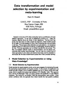
test input points [4]. However, this assumption is not fulfilled, for example, in interpolation or extrapolation scenarios: only few (or no) training input points exist in the regions of interest, implying that the test distribution is significantly different from the training distribution. Active learning also corresponds to such cases because the locations of training input points are designed by users while test input points are provided from the environment [1]. The situation where the training and test distributions are different is referred to as the situation under the covariate shift [3] or the sample selection bias [2]. Let px (x) (> 0) be the probability density function of training input points {xi }ni=1 . An example of an extrapolation problem where px (x) 6= pt (x) is illustrated in Figure 1. When px (x) 6= pt (x), two difficulties arise in a learning process. The first difficulty is parameter learning. The ordinary least-squares learning, given by " n # ´2 X³ ˆ min f (xi ) − yi , (3) α
i=1
tries to fit the data well in the region with high training data density. This implies that the prediction can be inaccurate if the region with high test data density has low training data density. Theoretically, it is known that when the training and test distributions are different and the true function is not realizable (i.e., the learning target function is included in the model at hand), least-squares learning is no longer consistent (i.e., the learned parameter does not converge to the optimal one even when the number of training examples goes to infinity). This problem can be overcome by using a least-squares learning weighted by the ratio of test and training data densities3 [3]. " n # ´2 X pt (xi ) ³ ˆ min f (xi ) − yi . (4) α p (xi ) i=1 x A key idea of this weighted version is that the training data density is adjusted to the test data density by the density ratio, which is similar in spirit to importance sampling. Although the consistency becomes guaranteed by this modification, the weighted least-squares learning tends to have large variance. Indeed, it is no longer asymptotically efficient even when the noise is Gaussian. Therefore, in practical situations with finite samples, a stabilized estimator, e.g., " n µ # ´2 X pt (xi ) ¶λ ³ min for 0 ≤ λ ≤ 1 (5) fˆ(xi ) − yi α p (x ) x i i=1 would give more accurate estimates4 . Note that λ = 0 corresponds to the ordinary least-squares learning (3), while λ = 1 corresponds to consistent weighted 3
4
In theory, we assume that px (x) and pt (x) are known. Later in experiments, they are estimated from the data and we evaluate the practical usefulness of the theory. ˆ λ obtained by the weighted least-squares learning (5) The learned parameter ˆ λ = Lλ y , where Lλ = (X > D λ X )−1 X > D λ , X i,j = ϕj (xi ), D is given by is the diagonal matrix with the i-th diagonal element pt (xi )/px (xi ), and y = (y1 , y2 , . . . , yn )> .
Fig. 1. An illustrative example of extrapolation by fitting a linear function fˆ(x) = α1 + α2 x. [Left Input Densities 1 column]: The top graph depicts 0.5 0.2 the probability density functions of 0 −0.5 0 0.5 1 1.5 2 2.5 3 the training and test input points, 0 px (x) and pt (x). In the bottom 0 0.2 0.4 0.6 0.8 1 λ=0 (Ordinary LS) 1 three graphs, the learning target "Large Bias" 0.5 function f (x) is drawn by the solid 10−fold Cross−Validation f(x) 0 1.5 fhat(x) line, the noisy training examples are Training −0.5 Test plotted with ◦’s, a learned function 1 −0.5 0 0.5 1 1.5 2 2.5 3 fˆ(x) is drawn by the dashed line, 0.5 and the (noiseless) test examples λ=0.5 (Intermediate) 1 "Balanced" are plotted with ×’s. Three differ0.5 0 ent learned functions are obtained 0 0.2 0.4 0.6 0.8 1 0 by weighted least-squares learning −0.5 with different tuning parameter λ. Proposed Estimator −0.5 0 0.5 1 1.5 2 2.5 3 0.4 λ = 0 corresponds to the ordinary λ=1 (Consistent) least-squares learning (small vari1 "Large Variance" 0.2 0.5 ance but large bias), while λ = 1 0 gives an consistent estimate (small −0.5 0 bias but large variance). With finite −0.5 0 0.5 1 1.5 2 2.5 3 0 0.2 0.4 0.6 0.8 1 samples, an intermediate λ, say λ = λ x 0.5, often provides better results. [Right column]: The top graph depicts the mean and standard deviation of the generalization error over 300 independent trials, as a function of λ. The middle and bottom graphs depict the means and standard deviations of the estimated generalization error obtained by the standard 10-fold cross-validation (10CV) and the proposed method. The dotted lines are the mean of the true generalization error. 10CV is heavily biased because of px (x) 6= pt (x), while the proposed estimator is almost unbiased with reasonably small variance. 1.5
px(x): Training pt(x): Test
0.4
True Generalization Error
least-squares learning (4). Thus, the parameter learning problem is now relocated to the model selection problem of choosing λ. However, the second difficulty when px (x) 6= pt (x) is model selection itself. Standard unbiased generalization error estimation schemes such as crossvalidation are heavily biased, because the generalization error is over-estimated in the high training data density region and it is under-estimated in the high test data density region. In this paper, we therefore propose a new generalization error estimator. Under covariate shift, the proposed estimator is proved to be exactly unbiased with finite samples in realizable cases and asymptotically unbiased in general. Furthermore, the proposed generalization error estimator is shown to be able to accurately estimate the difference of the generalization error, which is a useful property in model selection. For simplicity, we focus on the problem of choosing the tuning parameter λ in the following. Note, however, that the proposed theory can be easily extended to general model selection of choosing basis functions or regularization constant.
2
A New Generalization Error Estimator
Let us decompose the learning target function f (x) into f (x) = g(x) + r(x), where g(x) is the orthogonal projection of f (x) ontoRthe span of {ϕi (x)}pi=1 and the residual r(x) is orthogonal to {ϕi (x)}pi=1 , i.e., r(x)ϕi (x)pt (x)dx = 0. Since is included in the span of {ϕi (x)}pi=1 , it is expressed by g(x) = Pp g(x) ∗ ∗ ∗ ∗ > ∗ i=1 αi ϕi (x), where α = (α1 , α2 , . . . , αp ) are unknown optimal parameters. R Let U be a p-dimensional matrix with the (i, j)-th element U i,j = ϕi (x)ϕj (x)pt (x)dx, which is assumed to be accessible in the current setting. Then the generalization error J is expressed as Z Z Z 2 ˆ ˆ J(λ) = fλ (x) pt (x)dx − 2 fλ (x)f (x)pt (x)dx + f (x)2 pt (x)dx ˆ λ, α ˆ λ i − 2hU α ˆ λ , α∗ i + C, = hU α (6) R ˆ λ, α ˆ λ i is accessible and where C = f (x)2 pt (x)dx. In Eq.(6), the first term hU α the third term C does not depend on λ. Therefore, we focus on estimating the ˆ λ , α∗ i”. second term “−2hU α Hypothetically, let us suppose that the following two quantities are available. (i) A matrix Lu which gives a linear unbiased estimator of the unknown true parameter α∗ : E² Lu y = α∗ , where E² denotes the expectation over the noise {²i }ni=1 . (ii) An unbiased estimator σu2 of the noise variance σ 2 : E² σu2 = σ 2 . Note that Lu does not depend on Lλ . Then it holds that ˆ λ , α∗ i = hE² U Lλ y, E² Lu yi = E² [hU Lλ y, Lu yi − σu2 tr(U Lλ L> E² hU α u )], (7) ˆ λ , α∗ i if which implies that we can construct an unbiased estimator of E² hU α Lu and σu2 are available. However, in general, neither Lu nor σu2 may not be available. So we use the following approximations instead: b u = (X > DX)−1 X > D L
and
c2 = kGyk2 /tr(G), σ u
(8)
b u corresponds to Eq.(4), which imwhere G = I − X(X > X)−1 X > . Actually, L b plies that Lu exactly fulfills the requirement (i) in realizable cases and asymptotically satisfies it in general [3]. On the other hand, it is known that the above c2 exactly fulfills the requirement (ii) in realizable cases [1]. Although, in general σ u c2 does not satisfy the requirement (ii) even asymptotically, it turns out cases, σ u c2 is not needed in the following. that the asymptotic unbiasedness of σ u Based on the above discussion, we define the following estimator Jˆ of the generalization error J. c2 tr(U Lλ L b u yi + 2σ b > ). ˆ J(λ) = hU Lλ y, Lλ yi − 2hU Lλ y, L u u
(9)
ˆ B² = E² [Jˆ − J] + C. Then we have the following Let B² be the bias of J: theorem (proof is omitted because of lack of space).
Theorem 1 If r(xi ) = 0 for i = 1, 2, . . . , n, B² = 0. If δ = max{|r(xi )|}ni=1 is 1 sufficiently small, B² = O(δ). If n is sufficiently large, B² = Op (n− 2 ). This theorem implies that, except for the constant C, Jˆ is exactly unbiased if f (x) is strictly realizable, it is almost unbiased if f (x) is almost realizable, and it is asymptotically unbiased in general. We can also prove that the above Jˆ can estimate the difference of the generalization error among different models. However, because of lack of space, we omit the detail.
3
Numerical Examples
Figure 1 shows the numerical results of an illustrative extrapolation problem. The curves in the right column show that the proposed estimator gives almost unbiased estimates of the generalization error with reasonably small variance (note that the target function is not realizable in this case). We also applied the proposed method to Abalone data set available from the UCI repository. It is a collection of 4177 samples, each of which consists of 8 input variables (physical measurements of abalones) and 1 output variable (the age of abalones). The first input variable is qualitative (male/female/infant) so it was ignored, and the other input variables were normalized to [0, 1] for convenience. From the population, we randomly sampled n abalones for training and 100 abalones for testing. Here, we considered a biased sampling: the sampling of the 4-th input variable (weight of abalones) has negative bias for training and positive bias for testing. That is, the weight of training abalones tends to be small while that for the test abalones tends to be large. We used multi-dimensional linear basis functions for learning. Here we suppose that the test input points are known (i.e., the setting corresponds to transductive inference [4]) and the density functions px (x) and pt (x) were estimated from the training input points and test input points, respectively, using a kernel density estimation method. Figure 2 depicts the mean values of each method over 300 trials for n = 50, 200, and 800. The error bars are omitted because they were excessive and deteriorated the graphs. Note that the true generalization error J is calculated using the test examples. The proposed Jˆ seems to give reasonably good curves and its minimum roughly agrees with the minimum of the true test error. On the other hand, irrespective of n, the minimizer of 10CV tend to be small. We chose the tuning parameter λ by each method and estimated the age of the test abalones by using the chosen λ. The mean squared test error for all test abalones were calculated, and this procedure was repeated 300 times. The mean and standard deviation of the test error of each method are described in the left half of Table 1. It shows that Jˆ and 10CV work comparably for n = 50, 200, while Jˆ outperforms 10CV for n = 800. Hence, the proposed method overall compares favorably to 10CV. We also carried out similar simulations when the sampling of the 6-th input variable (weight of gut after bleeding) is biased. The results described in the right half of Table 1 showed similar trends to the previous ones.
n = 50
J
13.5
n = 200
n = 800
13 12.5 12 11.5
8
7
7.8
6.8
J
11 0 14
0.2
0.4
0.6
0.8
1
0
10CV
0.2
0.4
0.6
0.8
1
10CV
0.2
0.4
0.6
0.8
1
0.4
0.6
0.8
1
10CV
6.5
7
10
0
7
8
12
J
7.2
8.2
6 6
8 0
0.2
0.4
0.6
0.8
1
Proposed
18
5.5 0
0.2
0.4
0.6
1
Proposed
11.2
17.5
0.8
16.5
9
10.6 0
0.2
0.4
λ
0.6
0.8
1
Proposed
9.2
10.8
16
0.2
9.4
11
17
0 9.6
0
0.2
0.4
λ
0.6
0.8
1
0
0.2
0.4
λ
0.6
0.8
1
Fig. 2. Extrapolation of the 4-th variable in the Abalone dataset. The mean of each method is described. Each column corresponds to each n. Table 1. Extrapolation of the 4-th variable (left) or the 6-th variable (right) in the Abalone dataset. The mean and standard deviation of the test error obtained with each method are described. The better method and comparable one by the t-test at the significance level 5% are described with boldface. n Jˆ 10CV Jˆ 10CV n 50 11.67 ± 5.74 200 7.95 ± 2.15 800 6.77 ± 1.40
4
10.88 ± 5.05 8.06 ± 1.91 7.23 ± 1.37
50 10.67 ± 6.19 200 7.31 ± 2.24 800 6.20 ± 1.33
10.15 ± 4.95 7.42 ± 1.81 6.68 ± 1.25
Conclusions
In this paper, we proposed a new generalization error estimator under covariate shift. The proposed estimator is shown to be unbiased with finite samples in realizable cases and asymptotically unbiased in general. Experimental results showed that model selection with the proposed generalization error estimator is compared favorably to the standard cross-validation in extrapolation scenarios.
References 1. V. V. Fedorov. Theory of Optimal Experiments. Academic Press, New York, 1972. 2. J. J. Heckman. Sample selection bias as a specification error. Econometrica, 47(1):153–162, 1979. 3. H. Shimodaira. Improving predictive inference under covariate shift by weighting the log-likelihood function. Journal of Statistical Planning and Inference, 90(2):227– 244, 2000. 4. V. N. Vapnik. Statistical Learning Theory. John Wiley & Sons, Inc., New York, 1998.