Tutorial. Three-dimensional Euclidean geometry can be modeled in several ways. .... 2 Illustration of the geometric computations that we treat in detail for each ...
Tutorial
Modeling 3D Euclidean Geometry T
Daniel Fontijne and Leo Dorst University of Amsterdam
he space we live in is well described as 3D Euclidean geometry for most computer graphics applications. Although it would seem straightforward to directly implement this for realistic-image generation and object simulation including their properties, most computer graphics programmers find a more indirect method attractive. That is, we prefer constructing a computational model of the 3D geometry to implement. This Three-dimensional Euclidean often improves programs in structure and efficiency. For example, geometry can be modeled in the widespread use of homogeneous coordinates, which uses a 4D linear algebra to perform some of several ways. We compare the 3D Euclidean geometry. But the vectors from 3D linear algebra also the elegance and have their uses, as do quaternions— which appear to live in a 4D comperformance of five such plex algebra—and even Plücker coordinates—which describe 3D models in a ray-tracing lines using an unfamiliar 6D space. In fact, the choice of models is getapplication. ting confusing. Explanatory papers often suggest different algebras for different aspects of geometry.1-4 Our programs typically reflect this approach. To many, the recently discovered geometric algebra appears to be just one more possibility, but there is another way of looking at this scheme.5-7 Instead, in geometric algebra we finally have a framework containing all these modeling options and approaches in an organized manner. This approach streamlines applications by assigning various tricks such as quaternions and Plücker coordinates to a proper geometric algebra of appropriate real, interpretable vector spaces. This article compares five models of 3D Euclidean geometry—not theoretically, but by demonstrating how to implement a simple recursive ray tracer in each of them. It’s meant as a tangible case study of the profitability of choosing an appropriate model, discussing the trade-offs between elegance and performance for this particular application. This article acts as a practical sequel to two tutorials on geometric algebra previ-
2
March/April 2003
ously published in IEEE CG&A, and we frequently reference those tutorials.5-6 The models we compare are ■ ■ ■ ■
■
3D linear algebra (3D LA); 3D geometric algebra (3D GA), which naturally absorbs the quaternions into 3D real geometry; 4D linear algebra (4D LA), that is, the familiar homogeneous coordinates; 4D geometric algebra (4D GA), implements the homogeneous model, which naturally absorbs Plücker coordinates of lines and planes into homogeneous computations; and 5D geometric algebra (5D GA), which implements the conformal model. This model gives coordinates to circles and spheres and provides the most compact expressions for 3D Euclidean computations known to date.
We picked both 3D LA and 4D LA because we wanted a basic and an advanced mainstream model as a baseline. We selected 3D GA and 4D GA because they are the (improved) GA variants of the 3D LA and 4D LA models. The 5D GA model demonstrates the possible improvements when using more sophisticated models. Although we don’t explicitly use Grassmann spaces as recommended by Goldman,2 we shall show that using geometric algebra to implement Grassmann spaces significantly extends their applicability. We choose a ray tracer as a benchmark for the following reasons: ■
■
■
Everyone familiar with computer graphics knows how a basic ray tracer works and possibly has implemented one. Implementing the core of a ray tracer is possible with a relatively small amount of code. This was important because we had to write many different implementations of the same algorithm. A ray tracer contains a diverse selection of geometric computations, such as rotation, translation, reflection, refraction, (signed) distance computation, and
Published by the IEEE Computer Society
0272-1716/03/$17.00 © 2003 IEEE
3D LA
3D GA
4D LA
4D GA
5D GA
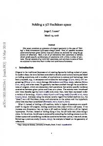
1 These images are identical, but we rendered each using a different 3D Euclidean geometry model. The scene consists of five objects—a transparent drinking glass, reflective sphere, red diffuse sphere, and textured/bump mapped wood piece—modeled with 7,800 triangles.
But we emphasize that our main goal here is to compare frameworks for representation and computation of geometry in some practical situation, not to build a ray tracer per se. The resulting ray tracer is not a marvel of contemporary computer graphics; yet it’s sufficiently sophisticated to render images such as those shown in Figure 1.
Ray tracer We use a basic recursive ray-tracing algorithm, without special techniques for efficiency, except for the use of a binary-space-partitioning (BSP) tree to accelerate raymesh intersection computations. Describing the precise algorithm in great detail is not meaningful here; only the geometric computations matter to the discussion at hand. A more detailed specification is available elsewhere (http://www.science.uva.nl/~fontijne/raytracer). The ray-tracing algorithm accepts as input a description of the scene, including camera, lighting, and polygonal model information such as position, orientation, shape; and material properties. For each image pixel, a ray is traced through the scene as it hits models and possibly gets reflected and refracted. Where a ray hits a surface, we perform lighting computations for each visible or ambient light source. The weighted sum of such lighting computations determines the final color of each pixel. The ray-tracing algorithm requires representations of geometric primitives such as vectors, points, lines, planes, spheres, as well as transformations of these primitives. In some models, primitives can also act as operators. For instance, using geometric algebra, a plane can be applied to another primitive directly to reflect that primitive in the plane. The geometric computations and operations that we must implement in each model to build our ray tracer are ■ ■ ■ ■ ■
rotation and translation of arbitrary primitives (points, lines, planes); reflection and refraction (Snell’s law) of directed lines; test for and computation of the intersection of lines and planes, lines and triangles, and lines and spheres; computation of the angle between lines and/or the angle between planes; and computation of the distance between two points and the signed distance of points to planes.
A
line-plane and line-sphere intersection. This lets us to show by example how to perform these computations in different models.
A (a)
(b)
(c)
(d)
(e)
2 Illustration of the geometric computations that we treat in detail for each model. Computation input is shown in black; output in gray. (a) Translation and rotation. (b) Intersection of a line and a plane. (c) Intersection of a line and a sphere. (d) Reflection of a directed line in a plane. (e) Refraction of a directed line in a plane. We do not give a detailed specification here of each of the geometric computations we discuss in this article. Writing down those descriptions implies the use of a specific model, because using a model is the only method we know to precisely encode geometry. An important theme of this article is that the use of any model, even a model of 3D Euclidean geometry, determines how you implement your solution and also shapes the way you think about the problem. To remain impartial with respect to the five models, we don’t use one of those models at this point to specify the geometric computations. Instead, we include a graphical representation in Figure 2. The icons in this figure show only the relevant geometric primitives. Derived geometric primitives such as angles, intermediate intersection points, and surface normals arise from the manner that we implement the computations in mainstream models of 3D Euclidean geometry and don’t necessarily arise in other models. For example, when we treat the model, a directed line can be reflected in a plane without using a surface normal or the intersection point of the line and the plane.
Models Our introductions to the five models show only how they represent some important primitives and rotation/translation operations. For the novel GA models, we give references to sources that provide more detail. After each introduction, we show the equations that implement the five geometric computations from Figure 2. Readers with little mathematical background shouldn’t be discouraged by these equations. Instead we encourage all readers not to focus on understanding the equations, but to read with a bird’s eye view and skip back and forth between the five sections to compare the
IEEE Computer Graphics and Applications
3
Tutorial
Mathematical Notations We employ the following notation across all models: lowercase Greek symbols (ρ, δ, φ) denote scalars. Lowercase bold symbols (u, q, s) represent elements of the algebra interpreted as geometric primitives (directions, points, spheres). Uppercase bold symbols (R, M) denote elements of the algebra interpreted as operators (rotors, transformation matrices). Lowercase plain symbols with an arrow r r overhead ( v, u) occasionally denote vectors that aren’t strictly elements of the algebra at hand. When possible, equations appear close to the form in which they are implemented in actual code.
length and simplicity of the equations and the number of split-up cases. Knowing that there exist alternative ways to implement each geometric operation in each model, we use the most obvious approach in each model. The equations we use to implement the geometric operations in the 3D LA model are virtually identical to those quoted in Glassner as most efficient.8 The “Mathematical Notation” sidebar defines the notations we use in the models.
3D linear algebra In the 3D LA model, vectors and scalars represent all primitives. A vector that points from the origin to the location of the point represents a point. A vector pointing from the origin to some point on a line and a unit vector pointing along the direction of a line represents a line. A normal vector and a scalar that gives the distance of the plane to the origin represent a plane. A vector pointing from the origin to the center of a sphere and a scalar giving the radius represents a sphere. We explicitly represent each primitive relative to a specific origin that we chose a priori. A vector represents translation. Because it’s a linear mapping, a 3 × 3 matrix represents rotation about the origin. We made all geometric computations using matrixvector multiplication, addition and subtraction of vectors, scalar multiplication, dot products (denoted by •), and cross products (denoted by ×). Rotation/translation. A point q is rotated/translated as q′ = Rq + t, where R is a rotation matrix, and t is a translation vector. To translate/rotate a line (given by point ql on the line and a unit vector u along the line), we compute q′l = Rql + t and u′ = Ru. A plane (given by its unit normal vector n and the scalar distance to the origin δ) is rotated/translated by n′ = Rn and δ′ = δ + t • n′ (http://carol.wins.uva.nl/~fontijne/raytracer/files/ raytracer_primitives.pdf and http://carol.wins.uva. nl/~fontijne/raytracer/files/raytracer_operations.pdf) Line-plane intersection. We can compute the intersection point qi of a line and a plane as qi = ql −
((ql • n ) − δ )u u•n
(1)
if u • n is not equal to 0. Line-sphere intersection. We can compute the two intersection points q− and q+ of a line and a sphere
4
March/April 2003
(given by its center point qs and its scalar radius ρ). First, the closest point qc to the center of the sphere on the line is computed as qc = ql + ((qs − ql) • u)u, then the normalized squared Euclidean distance, δ 2n of qc to qs determines if the line intersects the sphere: δ 2n =
(q c − q s ) • (q c − q s ) ρ2
If δ 2n is larger than 1, the line and the sphere do not intersect. If δ 2n is exactly 1, qc is the single intersection point. Otherwise q− and q+ can be computed as 2 q± = qc ± ρ 1 − δ n u
Reflection. The reflected direction u′ of a line in a plane, can be computed as u′ = −2(n • u)n + u
(2)
The reflected line would then be given by qi (the intersection point of the line and the plane) and u′. Note that we have to explicitly compute qi (using Equation 1) before we obtain a full representation of the reflected line. Snell’s law. As a ray travels from one medium to another, its direction gets refracted according to Snell’s law: sinφ1 sin φ2
=
η2 η1
where φ1 is the incoming angle, φ2 is the outgoing angle, and η1 and η2 are the refractive indices of the media. In the “Derivation of the 3D Geometric Algebra Refraction Equation” sidebar we use geometric algebra to compactly derive the classical equation for implementing Snell’s law. Here we only present the result of that derivation, translated to 3D LA. The unit surface normal of the (tangent-) plane separating the media is given by n. The unit direction of the line is given by u. We define η = η2 /η1, the refractive index of medium 2 relative to medium 1. This is all we need to compute the refracted direction of the line: u ′ = sign(n•u) 1 − η2 + (n•u)2 η2 − (n•u)η n + ηu (3)
3D geometric algebra Three-dimensional geometric algebra is an extension of 3D linear algebra.5,6 It has an operation to span subspaces through the origin: the outer product5 denoted by the ∧ symbol. Such subspaces or blades5 are the basic elements of computation. In 3D GA, we interpret the bivectors, or 2-blades, (of the form a ∧ b) as oriented, directed planes through the origin. We use bivectors instead of normal vectors because they encode the same information but behave better under linear transformations. We can naturally extend the inner product
Derivation of the 3D Geometric Algebra Refraction Equation We use 3D geometric algebra (3D GA) to derive 3D linear algebra (3D LA) Equation 3 (in the main article text), which we repeat here: u′ =
•
•
•
(A) (B) (C)
Equation A states that u, u′, and n must all lie in the same plane, while the sizes of both bivectors are related by the constant η. Equation B simply states that the lengths of u′ and u must be equal, while Equation C states that u′ and u must both have the same heading with respect to n. We will extract u′ from Equation A. The sum of the inner and outer product of u′ and n is equal to their geometric product u′n = u′ • n + u′ ∧ n
(E)
u′ ∧ n + u′ • n = ηu ∧ n + sign (u • n)
(F)
If we compare the left hand side of Equation F to the right hand side of Equation D, we see that Equation F is the (invertible) geometric product of u′ and n, so we divide by n to finish:
u′ =
If both n and u have unit length we can simplify this to u′ = = ηu + The last step is apply the fact
(D)
This suggests that, if we could express u′ • n without using u′, we could get the answer by adding u′ • n to Equation A’s left hand side and dividing by n. To find an expression for u′ • n, we note that n2u2 = n2u′2 = nu′u′n = (n • u′ + η(n ∧ u))(u′ • n + η (u ∧ n)) = (u′ • n)2 − η(u′ • u)(u ∧ n) + η(u′ • u) (u ∧ n) − η2(u ∧ n)2 = (u′ • n)2 − η2(u ∧ n)2
(denoted by the • symbol) to blades, and this is useful for projection and metric relationships. GA also has a geometric product,5 denoted by a half space symbol, as in ab. The geometric product permits multiplication and division5 by vectors and subspaces. The ratio of two vectors form a rotor,6 which we can use as a rotation operator. In fact, the rotor has the same properties as a quaternion, but within the context of geometric algebra, it’s a real operator that can rotate subspaces of any grade. Alternatively, we can construct a rotor as the exponential of the bivector representing the rotation plane and angle. Besides the various products, we also use addition, subtraction, and inversion. The dual operator,6 denoted by a superscript *, returns the dual of any blade, that is, the orthogonal complement in 3D space. These constructions naturally extend to n-dimensional vector spaces. Eight coordinates relative to an 8D basis can represent a general number or multivector in 3D GA: one for
u′ • n = sign(u ⋅ n) If we now add Equation E to Equation A we get:
You might compare this with work found in Glassner,1 which contains two 3D LA derivations of the same equation. In these equations, u is the direction of the incoming ray; n is the dual of the bivector p representing the plane, that is, the normal vector; and η = η1/η2 is a constant depending on the speed of light in both media. We compute u′, the direction of the outgoing ray. In 3D GA, Snell’s law can be fully specified by this set of equations: u′ ∧ n = ηu ∧ n u′2 = u2 sign(u′ • n) = sign(u • n)
From this and Equation C it follows that
(u ∧ n)2 = (u • n)2 − 1 This is the geometric algebra equivalent of −sin2φ = cos2φ−1.
Reference 1. A.S. Glassner, ed., An Introduction to Ray Tracing, Academic Press, 1989.
a scalar component, three for vector components, three for bivector components, and one for a trivector component (3-blades, interpreted as volume elements). Rotation/translation. We perform rotation of a vector about an axis through the origin in 3D GA with v′ = R v R−1. The vector is sandwiched between the rotor R and its inverse R−1. We create R as R = exp(−1/2φb) = cos1/2φ − b sin1/2φ, where φ is the angle of rotation and b the unit bivector denoting the plane of rotation. Such an R is normalized. This implies that R−1 is equal to R~, the reverse of R.5 We can efficiently compute the reverse by sign flipping part of the coordinates of R. Sandwiching operations like R v R−1 are common in GA; they typically apply objects like rotors to blades. Once you replace rotation matrix multiplication by this rotor sandwiching operation, points and lines are transformed the same way in 3D GA as in 3D LA. A plane is now given by its bivector b and its scalar
IEEE Computer Graphics and Applications
5
Tutorial
q2 × q2 O q2 – q2


![[EBOOKS] Euclidean Geometry in Mathematical ... - Google Sites](https://m.moam.info/img/260x300/ebooks-euclidean-geometry-in-mathematical-google-s_6477bacd097c474e708c0717.jpg)
