In this paper, a set of more than thirty parameters from seven distinct flight phases ... scatted flight data provide us a new way of modeling aircraft performance. By using ...... Journal of the American statistical Association, Vol. 46, No. 253, 1951, ... After obtaining his M.Sc. and pilots license in 1990, he started working at the ...
Twelfth USA/Europe Air Traffic Management Research and Development Seminar (ATM2017)
Modeling Aircraft Performance Parameters with Open ADS-B Data Junzi Sun, Joost Ellerbroek, Jacco Hoekstra Control and Simulation, Faculty of Aerospace Engineering Delft University of Technology Delft, The Netherlands
Abstract—Open access to flight data from ADS-B (Automatic Dependent Surveillance Broadcast) has provided researchers more insights for air traffic management than aircraft tracking alone. With large quantities of trajectory data collected from a wide range of different aircraft types, it is possible to extract accurate aircraft performance parameters. In this paper, a set of more than thirty parameters from seven distinct flight phases are extracted for common commercial aircraft types. It uses various data mining methods, as well as a maximum likelihood estimation approach to generate parametric models for these performance parameters. All parametric models combined can be used to describe a complete flight that includes takeoff, initial climb, climb, cruise, descent, final approach, and landing. Both analytical results and summaries are shown. When available, optimal parameters from these models are also compared with the Base of Aircraft Data and Eurocontrol aircraft performance database. This research not only presents a comprehensive set of methods for extracting different aircraft performance parameters but also provides a first part of open-source parametric performance models that is ready to be used by the ATM community. Keywords - Aircraft performance; Maximum likelihood estimation; ADS-B; Data mining
N OMENCLATURE to ic cl cr de fa ld
Aircraft Aircraft Aircraft Aircraft Aircraft Aircraft Aircraft
a∗ d∗ Vh,∗ Vcas,∗ R∗ M∗ H∗
Acceleration or deceleration Distance (takeoff or landing) Vertical speed Calibrated air speed Flight range Mach number Aircraft altitude
takeoff phase initial climb phase climb phase cruise phase descent phase final approach phase landing phase m/s2 km m/s m/s km km
I. I NTRODUCTION Aircraft performance models (APM) for ATM researches are commonly built based on manufacturer performance reports and/or recorded flight data. However, it is difficult for each researcher to obtain flexible access to these models and related data, as they are either costly or have certain license limitations. Even the most commonly used APM, Base of Aircraft Data family 3 (BADA3), has its license limitations [1]. BADA family 4 comes with even more strict license agreements, which make it very difficult to perform studies
that can be easily reproduced and compared within the research community. Thanks to the ICAO mandates on aircraft ADS-B equipment installation by 2020, an increasing number of commercial aircraft are being equipped with this capability. At the same time, many ground receivers are being installed around the world. Open flight data has become more and more accessible for every ATM researcher. Certain flight data such as position, altitude, velocity, and vertical speed of common aircraft types are broadcast and received constantly around the world by these ground receiver networks. These large amounts of scatted flight data provide us a new way of modeling aircraft performance. By using carefully designed data mining algorithms and statistical analyses, operational performance and limitation parameters of aircraft can be obtained from ADS-B flight data. In this paper, we are focusing on extracting complete operational and limitation models solely based on this open data approach. However, the biggest challenge is how to make use of these large quantities of data. As an aircraft performs differently in each flight phase, flight data need to be segmented accordingly. Machine learning and data mining methods, as proposed by Sun et al., have provided some efficient ways to process these loosely connected data points into organized segments based upon trajectory and respective flight phases [2]. As a continuation of this research, output data generated is further divided into detailed segments according to the model definitions that are proposed in this paper. In real flights, none of the two trajectories are identical. In every aircraft type, different levels of performance deviations are always present, and these values are often differ, even within the same phase of a flight. The main causes include aircraft mass, thrust settings, wind, and flight procedures. Errors in data can also contribute to these deviations. However, there is an underlying statistical model that can be used to describe these performance parameters. To identify the best mode, maximum likelihood estimators can be employed. The remainder of this paper is structured as follows. Section two introduces the model parameters, definitions, and maximum likelihood estimations for three different distribution functions. Section three explains the data and pre-processing methods. Section four is focused on methods and algorithms for constructing parameters of each flight phase. Detailed results on a single aircraft type and summaries of 17 different aircraft types are shown in section five. Finally, discussions
and conclusions are addressed in sections six and seven.
C. Probability distribution functions
II. M ODEL DEFINITIONS A. Parameters Similar to the flight phase definitions from ICAO Common Taxonomy Team [3], this research aims to derive performance parameters from the following flight phases: takeoff, initial climb, climb, cruise, descent, final approach, and landing. The significance of the performance indicators differs from one flight phase to another. For example, vertical velocity is only of interest during climb and descent, while during takeoff and landing, the runway distance, acceleration, and boundary velocities are of interest. Specifically, during the climb (or descent) phase, a constant CAS/Mach profile is extracted. Throughout the paper, the following parameters, shown in Table I, are defined and obtained accordingly. TABLE I P ERFORMANCE MODEL PARAMETERS Flight phase Takeoff Initial Climb
Performance parameters Vlof , dtof , a ¯tof Vcas,ic , Vh,ic
Cruise
Rcr , Rmax,cr , Hcr , Hmax,cr , Mcr , Mmax,cr
Landing
Hmach,cl ,
Rtop,de , Mde , Vcas,de , Hmach,cl , Vh,mach,de , Vh,cas,de , Vh,post-cas,de
(4) (5)
1 α−1 −y y e Γ(α)
(6)
1 y α−1 e−y k · Γ(α) x−µ y= k
p(y|φ) =
The maximum likelihood estimation (MLE) [4] is used to estimate the best unbiased value of a parameter (or a vector of parameters) based on observations. First, N observations X : {x1 , x2 , . . . , xn } are drawn from an unknown probability distribution function p(·) and characterized by a parameter vector φ, denoted {p(·|φ), φ ∈ Φ}. Then, assuming the sample observations are independent, the joint probability density, also known as the likelihood function of φ, denoted L(φ; ·), is expressed as follows:
L(φ ; x1 , . . . , xn ) = p(x1 , x2 , . . . , xN |φ) =
N Y
p(xi |φ) (1)
i=1
The maximum likelihood estimate of φ, denoted φˆMLE , is the φ vector that maximizes the likelihood. To simplify the calculation, the log-likelihood function is used:
arg max φ∈Φ
N Y i=1
arg max log( φ∈Φ
arg max φ∈Φ
N Y
i=1 N X i=1
p(x|φ) =
1 xα−1 (1 − x)β−1 B(α, β)
(8)
where B(α, β) is defined as: B(α, β) =
Γ(α)Γ(β) Γ(α + β)
(9)
In a general form where x ∈ (−∞, +∞), the location (µ) and scale (k) parameters are also introduced: p(y|φ) =
# p(xi |φ))
log[p(xi |φ)]
(7)
ˆ does not have a close The MLE estimator φˆMLE : (ˆ α, µ ˆ, k) form solution, but it can be solved numerically [5]. 3) Beta distribution: For a standardized Beta distribution with 0 < x < 1, the density function is:
1 y α−1 (1 − y)β−1 k · B(α, β) x−µ y= k
p(xi |φ)
"
=
(3)
where the α (α > 0) represents the shape of the distribution. In a general form where x ∈ (−∞, +∞), the location (µ) and scale (k) parameters are introduced:
Vapp , dbrk , a ¯brk
=
(x−µ)2 2σ 2
2) Gamma distribution: For a standardized Gamma distribution with y ∈ (0, +∞), the density function is expressed:
Hcas,cl ,
Vcas,f a , Vh,f a
=
2σ 2 π
e−
where the unknown PDF parameters φ : (µ, σ 2 ) represent the mean and variance. The MLE estimator φˆMLE can easily be found for a Normal distribution, with the mean and variance as the observation data:
p(y|φ) =
B. Estimation method
φˆMLE
1
¯ X n 1X ¯ 2 (xi − X) σ ˆ2 = n i=1
Rtop,cl , Vcas,cl , Mcl , Hcas,cl , Vh,pre-cas,cl , Vh,cas,cl , Vh,mach,cl
Final Approach
p(x|φ) = √
µ ˆ=
Climb
Descent
Three continuous probability distribution functions (PDF) are assumed for each of the performance parameters, which are Normal, Gamma, and Beta distributions. Then MLE is applied to obtain the best estimates φˆMLE for each PDF from sample data. 1) Normal distribution: For a Normal distribution, the density function is expressed:
(2)
(10)
Similar to Gamma distribution, it also does not have a closeˆ µ ˆ which needs form solution for the optimal φˆMLE : (ˆ α, β, ˆ, k), to be solved numerically [6].
4) Model fitness evaluation: After all possible optimal probability distribution models are computed, the best model of all three need to be identified. The Kolmogorov-Smirnov (KS) Test [7] is applied to obtain such a model. This test compares the cumulative distribution function (CDF) of a statistical model, denoted F (x), against the empirical distribution function (EDF) from the data, denoted Fn (x), and then generates the KS statistic D:
For deterministic calculations, ψˆ is recommended. However, any value from the interval [ψmin , ψmax ] is also applicable. For simulations that study the uncertainties, multiple values of a parameter can be drawn from the distribution, which would resemble the real world air traffic situation. It is important to note that certain errors may be present in flight data, such as inaccurate estimated wind speed or errors contained in GPS positions. Trajectory data need to be well processed in the first place.
D = max|Fn (x) − F (x)|
III. DATA PREPARATION
(11)
x
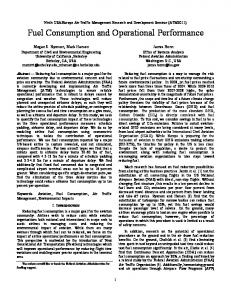
which represents the largest distance between F (x) and Fn (x). Of all three KS statistics DN , DΓ , and DB , the probability distribution that yields the minimum D will be selected. In practice, simple Normal distribution is always more favorable than Gamma or Beta distribution, due to its simplicity. Thus, a small margin is applied to prefer DN over DΓ or DB . An example data set of one parameter (takeoff acceleration) is shown in Fig. 1, 1.0 data norm (D: 0.04) gamma (D: 0.06) beta (D: 0.03)
Desnsity
0.8 0.6 0.4 0.2 0.0 1.0
1.2
1.4
1.6 1.8 2.0 Parameter values
2.2
2.4
2.6
Fig. 1. Comparison of three CDF with data EDF
A. Data source For this research, the input data are primarily based on ADSB messages that are broadcast by airplanes through ModeS transponders. However, even with good installation and placement, a single ground based receiver only has a maximum reception range of around 250nm (∼ 500km). Considering Mode-S line-of-sight availability, it is not possible to capture large quantities of completed flight data with a single ground station. It is especially challenging when dealing with long range aircraft. Thanks to networks of ADS-B ground receivers, such as FlightRadar24 [8], it is possible to gain access to a much larger scale of flight data collected from other ground stations from contributors around the world. It is also worth noting that in addition to ADS-B data, using the same receiver setup, aircraft positions, and velocities can be obtained from multiple ground stations using ModeS multilateration. The technology is also deployed by some ground receivers within the FlightRadar24 network. It is useful for those aircraft that are not yet equipped with ADS-B out equipment. However, the availability is limited to areas where ATC is presented and not useable when aircraft are close to the ground. B. Trajectory data process
where the CDF of all three models obtained from MLE are displayed against the EDF computed from the data. The best model (beta) is obtained by comparing D. The final selected PDF are illustrated in the third plot of Fig. 9. D. Parameter expression For each parameter in Table I, the following expression is constructed: ˆ ψmin , ψmax , ∗pdf } {ψ,
(12)
where the first three values are the optimal, minimum, and maximum values of such a parameter. The min and max values are obtained from a confidence intervals: 0.8 for most of the velocity parameters, 0.98 for range parameters, and 0.9 for other parameters. The probability density functions are provided as ∗pdf for the cases where parameter values need to be drawn from a probability distribution. Depending on the KS test, optimal ∗pdf is expressed as follows: 0 0 f or x ∼ N [ norm , µ, σ] 0 ∗pdf = [ gamma0 , α, µ, k] f or x ∼ Γ 0 [ beta0 , α, β, µ, k] f or x ∼ B
Data collected from ADS-B are usually scattered. Previous machine learning methods in [2] have made it possible to extract flight trajectory easily. However, this method can only segment flights into four different phases: on-ground, climb, cruise, and descent. For the research needs of this paper, further processing of those segments is employed. Firstly, an altitude threshold is applied on the climb and descent trajectory to extract initial climb and final approach. Secondly, a cruise buffer is introduced to distinguish the level-flight segments in climb or descent phases from cruise. Lastly, an evaluation process is used to examine the data of all flight segments, ensuring a certain level of completeness and continuity in the given time series data. The ground velocity information from ADS-B measurements are also integrated with meteorological data using interpolation models described in [2] to produce the true airspeed (TAS) of aircraft at any given location. TAS is then converted to calibrated airspeed (CAS) and Mach number under standard atmospheric conditions. IV. M ODEL CONSTRUCTION METHODS
(13)
After these flight trajectories are sorted and segmented by proper flight phases, they are ready to be used for constructing
desired model parameters. For each aircraft type, at least five thousand trajectories are used to give a good level of confidence in the model. This section discusses in detail the methods for extracting these parameters from the trajectory data. A. Takeoff During the takeoff phase, the parameters of most interest are takeoff distance (dtof ), average acceleration (¯ atof ), and lift-off speed (Vlof ). To overcome large noise in velocity measurements during the takeoff, a spline filter is applied to obtain a smoothed velocity sample set. After the smoothed time series data is computed, distance parameters can be derived from aircraft surface position at the starting and ending positions of the takeoff, using the spherical law of cosines:
The parameters to be studied are aircraft calibrated airspeed (Vcas,ic ) and vertical rate (Vh,ic ). Both parameters can be computed directly from ADS-B data. C. Climb The climb segment starts when the aircraft reaches clean configuration and lasts until the moment when it reaches cruise altitude. As a common practice, aircraft first accelerate to a target CAS and then fly according to this constant CAS. As the altitude of an aircraft increases, the speed of sound decreases, which results in an increasing Mach number. When a certain Mach number is reached, an aircraft will fly according to this constant Mach number until its cruising altitude. During the Mach climb segment, a decreasing CAS will be observed due to the decreasing air density. The climb CAS profile can be generalized in Fig. 3. 400
dtof = d1,N = R · arccos[sin γ1 · sin γN
350
(14)
a ¯ = argmin a ¯
i=1
ns
t. M ac
h
200 150
b Clim
100
(¯ a · (ti − t0 ) − vi )
2
(15)
Compared to the previous two parameters at takeoff, lift-off speed is more complicated to estimate, due to the low data update rate. There is usually a gap of several seconds between the last on-ground data and the first in-air data. {h1, Vh1} {V0, alof} t1
tlof
t0
Co
250
VCAS
where γ and λ represent the latitude and longitude in radians. Average acceleration a ¯tof can be obtained accurately from velocity measurements: N X
Const. CAS
300
+ cos γ1 · cos γN · cos(λN − λ1 )]
Fig. 2. Estimate the lift-off moment
To estimate the exact moment of lift-off, as shown in Fig. 2, a bi-directional extrapolation is used. Firstly, the vertical rate Vh and time stamp at the first in-air data are used to estimate the time of lift-off tlof . Combining this result with previously calculated a ¯tof , the lift-off speed can be obtained as follows: h1 Vh1 − t0 )
tlof = t1 − Vlof = V0 + a ¯tof · (tlof
(16) (17)
B. Initial climb The initial climb phase is defined as the segment from 35 f t until the aircraft reaches around 1500 f t. There are several major configuration changes (landing gear and flaps) during this short period of time that can affect the performance. However, the initial climb segment lasts for a short time in respect to the entire flight path. Thus, it suffers from relatively low data samples comparable to the takeoff phase.
50 0
Fig. 3. Standard climb profile
The challenge is to identify the crossover of this constant CAS/Mach climb. Knowing the general profile of CAS and Mach number during the climb, it is possible to design a twostep and two-piecewise estimator for extracting this feature from CAS and Mach number profiles. The estimator consist of two parts: an increasing (quadratic or linear) segment and a constant segment. The quadratic increasing part is designed so that it resembles the general observation of velocity increase with a decreasing acceleration. The constant segment approximates constant CAS or Mach values. The estimator is expressed as follows:
fmach (t)
=
fcas (t)
=
( k1 · (t − tmach )2 + ymach t ≤ tmach (18) ymach t ≥ tmach ( −k2 · (t − tcas )2 + ycas t ≤ tcas (19) ycas tcas ≤ t ≤ tmach
To illustrate this knowledge retrieving process, this two step piecewise least squared fitting can be described in the diagram of Fig. 4. The entire climbing phase in terms of Mach number can be divided in two parts (increasing and constant). The first estimator applies on the entire climb data and uses the leastsquare fitting to extract the best CAS/Mach transition time tmach and constant Mach climb number ymach . The second estimator uses tmach as cutoff time, fitting the remainder of the time series where Mach number is
D. Cruise
GS Wind Model
Mach
Fit: fmach(t)
ymach
tmach
TAS
Fit: fcas (t)
CAS
Validator ycas CAS/Mach
tcas
Fig. 4. Constant CAS/Mach climb identification process
increasing. This similarly structured estimator is used to obtain the constant CAS speed ycas and its starting time tcas . The final validation step takes into account k1 , k2 , and all four output parameters: tcas , ycas , tmach , and ymach to ensure the following boundary conditions:
Aircraft generally cruise at selected optimal altitudes. Parameters that are of interest for performance are extracted from the trajectories, such as the standard cruise altitude Hcr and Mach number Mcr . The limitations of aircraft such as cruise ceiling Hmax,cr and maximum cruise Mach number Mmax,cr can also be found. In addition, typical cruise range Rcr is extracted as an operational reference parameter. Since aircraft rarely flight directly between original and destination airports, the flight range cannot be calculated as the great circle distance between origin and destination. On the other hand, due to the measurement noise inherited from on-board GPS receivers, position reports in ADS-B can contain errors. When integrating positions along the trajectory, the accumulated error grows even larger. Hence, a filter is first implemented, and then the entire trajectory is re-sampled for integrating the cruise range. Such a process can be illustrated in Fig. 6, where the filtered trajectory is shown in red as compared to real position reports in blue and the direct path in dashed black line. 100◦ E
t0 < tcas < tmach < tN
105◦ E
110◦ E
115◦ E
120◦ E
30◦ N
30◦ N
25◦ N
25◦ N
20◦ N
20◦ N
15◦ N
15◦ N
10◦ N
10◦ N
CASmin < ycas < CASmax M achmin < ymach < M achmax k1 > 0 k2 > 0
(20)
40k
100◦ E
30k
105◦ E
110◦ E
115◦ E
120◦ E
20k 10k
Mach
CAS (kt)
altitude (ft)
To illustrate this entire process, this method is applied on one flight and shown in Fig. 5. The green and red colors represent the Mach and CAS profile during the climb, both with a constant part that has been identified by the model.
Fig. 6. Cruise range spline filtering
0 400 300
E. Descent
200
The descent phase of the aircraft is comparable to the climb phase. From the top of descent, the aircraft undergoes a constant Mach and constant CAS descent segment before reaching the approach altitude, as illustrated in Fig. 7.
100 0 1.0 0.8 0.6 0.4 0.2 0.0 0.0
Top of descent
0.2
0.4 0.6 time (scaled)
0.8
1.0
Fig. 5. Constant CAS/Mach climb identification example
After tcas and tmach are determined, transition altitudes Hcas,cl , Hmach,cl , at which the constant CAS and constant Mach climbing commence can be obtained. Vertical rates Vh,pre-cas,cl , Vh,cas,cl , Vh,mach,cl that correspond to these three segments can also be computed. In addition, range from takeoff to the top of climb Rtop,cl is calculated.
Const. Mach
Const. CAS
Final Approach
Fig. 7. Standard descent profile
The essential parameters to be modeled are: range from top of descent to destination Rtod,de , constant Mach vmach,de , constant CAS vcas,de , crossover altitudes Hmach,de and Hcas,de , and vertical speed Vh,mach,de , Vh,cas,de , and Vh,post-cas,de . Similar to climb, the constant Mach/CAS descent performance can be modeled by piecewise estimators. It is possible to use the same process as described in Fig. 4. The Mach profile is described using two linear pieces. The CAS profile consists of a linear and quadratic piece due to the high nonlinearity in speed at the final approach segment. The model can be described as follows: ( fmach (t)
= (
fcas (t)
=
ymach −k1 · (t − tmach ) + ymach −k2 · (t − tcas )2 + ycas ycas
t ≤ tmach (21) t ≥ tmach
t ≤ tcas (22) tcas ≤ t ≤ tmach
40k 30k
CAS (kt)
V. R ESULTS A set of 17 common aircraft types are studied in this research. Sufficient data are collected for all aircraft. For each aircraft type, around 5000 sets of data per flight phase are considered. In order to better illustrate the modeling of each individual parameter, detailed results from a single aircraft type (Airbus A320) are described according to the previous model specification. Results for other aircraft types are shown in a combined table. A. Airbus A320 For each parameter, all three probability density functions (Normal, Gamma, and Beta) are applied using MLE. The best model is chosen and represented by different colors in all ˆ ψmin , figures, shown in red, green, and blue respectively. ψ, and ψmax are also marked in each of the plots accordingly. 1) Take-off: Three performance parameters dtof , Vlof , and a ¯tof are shown in Fig. 9, where the optimal values of these parameters are 1.68km, 84m/s (∼ 163kt), and 1.88m/s2 .
20k
Takeoff dist. (km)
10k
Mach
altitude (ft)
Similarly, the result of such model as applied on one flight is shown in Fig. 8.
be observed from the last in-air velocity. Similar to takeoff, breaking distance can be calculated using Equation 14, and average deceleration can be calculated from Equation 15.
0 1.0 0.8 0.6 0.4 0.2 0.0 400
Liftoff speed (m/s) vlof
dtof
1.08
1.68
2.28
70.4
85.3 96.9
Mean accelaration (m/s2 ) a ¯tof
300 200
1.40
100 0 0.0
0.2
0.4 0.6 time (scaled)
0.8
1.0
Fig. 8. Constant CAS/Mach descent identification example
During descent, it is common for aircraft to follow a certain Continuous Descent Approach (CDA), eliminating level-flight segments so as to reduce fuel consumption and engine noise. Such an approach affects the result of descent performances. This factor is discussed in section VI-C in this paper. F. Final Approach Due to different control procedures at each airport, it is not easy to generalize the entire approach segment solely based on flight data. However, the final approach segment from around 1000 ft until landing can be modeled. The segment of final approach represents the end of a descent, where aircraft operate at a constant airspeed and rate of descent. The approaching speed vcas,f a and Rate of descent vh,f a are modeled. G. Landing The landing model is comparable with the take-off model. Parameters such as: approaching velocity Vapp , braking distance dbrk , and deceleration abrk of the aircraft are modeled similar to the takeoff phase. Approaching speed Vapp can
1.95 2.28
Fig. 9. Take-off parameters
2) Initial climb: Two performance parameters Vcas,ic and Vh,ic of the initial climb, up to the altitude of 1500ft, are shown in the first two plots of Fig. 10, where the most likely values are 81m/s (∼ 157kt) and 12.4m/s (∼ 2440f pm) Mean airspeed (m/s)
Mean vertical rate (m/s)
Vh,ic
70
81
92
Std. of airspeed (m/s) 0.77 Vh,std,ic
0.37
5.13
Vcas,ic
8.72
12.78 15.72
Std. of vertival rate (m/s) 1.60 Vcas,std,ic
0.50
5.40
Fig. 10. Initial climb parameters
The evidence for quasi-constant airspeed and vertical rate assumption can be seen from the standard deviations per trajectory, shown in the last two plots. It should also be noted that, in general, the vertical rate has larger variances. This is due to the fact that data sources for vertical rate commonly contain certain level of uncertainties as suggested in [9].
3) Climb: Within the climb phase, the objective is to model the constant CAS/Mach climbing profile, as well as the vertical rates in each of the segments of the profile. All parameters are shown in Fig. 11. Before the aircraft accelerates to a constant calibrated airspeed of 153 m/s (295 kt), it has a mean climbing rate of 10.32 m/s (2000 f pm), once reaching the transition altitude of approximately 4.8 km (16k f t). The aircraft then climbs at 8.5 m/s (1670 f pm) until reaching the constant Mach number 0.77 at an altitude of 7.7 km (25k f t). After that, the aircraft climbs at 5.44 m/s (1060 f pm) until reaching the cruise altitude. The flight range of the climb phase is also shown in the last plot, which is typically around 246 km. Constant CAS (m/s)
Constant Mach (-)
in the dataset is around 4700 km, which is closer to its claimed maximum flight range (6500km) if taking into account climb, descent range, and fuel reserves. 5) Descent: Similar to climb, the descent phase can also be modeled as a constant Mach descent segment and a constant CAS descent segment. The parameters are shown in Fig. 13. The aircraft starts initial descent at constant Mach number 0.77 and vertical rate −6.3 m/s (−1240 f pm) until reaching an altitude of 9.4km (31k f t). It then starts a constant CAS descent of 150 m/s (290 kt) and vertical rate of −9.7 m/s (−1900 f pm) until reaching the altitude 5.3km (17k f t). Then, the aircraft descends with a vertical rate at −5.9m/s (−1160 f pm) until final approach. The last plot shows the range from top-of-descent to destination, typically around 230km.
Mcl
Vcas,cl
Constant Mach (-) 136
155
170
0.68
0.77
0.86
Trans. alt. cst.-CAS (km)
Trans. alt. cst.-Mach (km)
Hcas,cl
Hmach,cl
Mean RoD, cst.-Mach (m/s) Mde
0.67
0.77 0.86
Trans. alt. cst.-Mach (km) 2.2
4.8
7.4
5.4
7.8
Mean RoC, cst.-CAS (m/s)
Vh,precas,cl
Vh,cas,cl
7.71
10.32 12.93
Mean RoC, cst.-Mach (m/s)
5.56
8.60
6.6
9.4 10.6
7.32
Rtop,cl
169 246
117
134
151
Mean cruise altitude (km) Hcr
10.0
10.9
11.8
132
150
168
Trans. alt. cst.-CAS (km) Hmach,de
-14.36 -9.73
-5.10
-7.83
Mean cruise Mach (-) Mcr
0.71
0.78
0.86
Cruise range (km) 932
473
Rmax,cr
3819
Fig. 12. Cruise parameters
Unlike other performance parameters, the cruise range Rcr is spread very widely, where 98% of flights globally range from 473 km to 3819 km. This can reflect the wide ranging usage of the A320. However, most common flights cruise with range around 1000 km operationally. The maximum range presented
2.5
-5.88
-3.94
5.3
8.2
Descent range (km)
Vh,postcas,de
391
4) Cruise: During the cruise phase, cruise speed Vcas,cr , Mach number Mcr , altitude Hcr , and cruise range Rcr are shown in Fig. 12 respectively. Maximum cruise Mach number Mmax,cr and maximum cruise altitude Hmax,cr can be obtained as the maximum value of Mcr and Hcr .
Vcas,cr
Vcas,de
Vh,mach,de
11.65
Fig. 11. Climb parameters
Mean cruise CAS (m/s)
Constant CAS (m/s)
Mean RoD, cst.-CAS (m/s)
Mean RoD, after-CAS (m/s) 5.44
-1.98
Climb range (km)
Vh,mach,cl
3.87
-13.03 -7.51
Hcas,de
9.7
Mean RoC, pre-CAS (m/s)
Vh,cas,de
234
181
Rtop,de
424
Fig. 13. Descent parameters
It is worth taking into consideration that the results obtained from the dataset contain both CDA and non-CDA descent approaches. 6) Final Approach: At final approach, airspeed Vcas,f a and vertical rate Vh,f a are shown in Fig. 14, which are 69 m/s (134 kt) and −3.54 m/s (−700 f pm) respectively. The last two plots show the variance of these two parameters within each trajectory. Similar to the initial climb, the quasi-constant airspeed and vertical rate assumption is still valid. 7) Landing: At the final flight landing phase, approach speed Vapp , breaking distance dbrk , and mean deceleration a ¯brk are shown in Fig. 15, with values of 68 m/s (132 kt), 1.2 km, and −1.07m/s2 . Breaking distance shows a large variance, ranging from around 600 meters to 3km. Different factors such as aircraft weight, wind direction, and runway conditions would all cause such large deviations. B. Multiple aircraft types The same methods and analysis are applied on a much larger dataset that contains multiple aircraft types. Due to the complexity of displaying all distribution and models from each
Mean airspeed (m/s)
Mean vertical rate (m/s)
Vcas,f a
59
69
80
-4.17
Std. of airspeed (m/s) 0.78 0.47
Vh,f a
-3.54
-2.90
Std. of vertival rate (m/s) 0.51
Vcas,std,f a
6.44
0.25
Vh,std,f a
1.40
Fig. 14. Final approach parameters
with the exception that takeoff distance (Vtof ) is around 20% lower than for BADA. This is likely due to the maximum takeoff weight assumed in the BADA model. If the maximum values of the parameter Vlof |max from this paper are used, the result becomes comparable with BADA. In a similar fashion, the Eurocontrol Aircraft Performance Database [11] can also be used as a source of comparison. It provides more performance parameters that are used primarily for training purposes on a wide range of commercial and military aircraft. A total of 17 parameters from 14 aircraft that exist in both models are compared. The result is shown in Fig. 17:
Breaking distance (km) dbrk 1.20
Approach speed (m/s) Vapp
60
0.63
3.30
Mean breaking acc. (m/s ) a ¯brk 2
-0.44
−20
parameters per aircraft type, the optimal parameter values of 17 aircraft types are shown in Table II. VI. VALIDATIONS AND DISCUSSIONS A. Validation of performance parameters The performance parameters described in this paper are all derived from large numbers of flight data, which resemble the best estimates of how aircraft truly perform. There are a few existing performance models that can be used as references to examine the validity of the estimated parameters. Within the BADA family 3 [10], similar performance parameters are contained in the OPF (Operational Performance File) and APF (Airline Procedure File). The difference between BADA and our model on ten performance parameters (from 14 aircraft types) are shown in Fig. 16.
V
V
rk
db
h, h, de ca s, de h, po st ,d V e ap p
de
ac h, m
V
de
V
,c
Mr
cr
M
ax m
H
l
r ,c
h, c
ax
ac
m
m h,
R
cl
V
V
h, ca
s, cl
cl
e,
V
h, pr
s,
V
vl
M
−60
Fig. 15. Landing parameters
cl
−40
ca
-1.18
0
of
-1.91
20
of
68.1 77.3
dt
55.8
Difference in %
40
Fig. 17. Comparison with Eurocontrol Aircraft Performance Database
The parameters that are displayed with large bias are vertical rates during the descent phase. In the Eurocontrol database, it is common that the second descent segment has much higher vertical rate. However, this trend is not significant in the flight data as observed. It can also be the case that the transition altitudes obtained from data in this paper are different from the fixed transition altitude from the Eurocontrol database. Furthermore, compared to both BADA and the Eurocontrol database, the models obtained in this paper also include the minimum value, maximum value, and a parametric model for each parameter. This accuracy comes as an additional advantage for large-scale ATM simulators such as BlueSky simulator [12]. B. Point of lift-off and touch-down
Difference in %
40 20 0 −20 −40 l l d tof V cas,c M c
M cr
r x,c
r
x,c
V ma M ma H ma
r x,c
V de
Md
e
d br k
Fig. 16. Comparison with BADA
It can be observed that most parameters from different aircraft types are very close to what is presented in BADA,
During the takeoff and landing phases, due to a low data update rate, an estimation method in Fig. 2 is used to locate the most likely lift-off or touch-down moment, from which related parameters are interpolated. Statistically, there are relatively large gaps between the last on-ground data and first in-air data. The time gaps ∆t are measured from a large number (around 7000 flights) of takeoffs and landings, as shown in Fig. 18. Most commonly, the ∆t is about three to nine seconds during which the aircraft would have flown, climbed, or descended for a fairly large distance. Thus, when dealing with such data, using the above method improves the accuracy of parameter estimations during the phases where fewer samples are available. It is also interesting to notice that there is a three-second time gap in both figures of take-off and landing. This is
TABLE II P ERFORMANCE MODEL FOR VARIOUS COMMERCIAL AIRCRAFT Unit
A319 A320 A321 A332 A333 A343 A388 B737 B738 B739 B744 B752 B763 B77W B788 B789 E190
TO
vlof dtof a ¯tof Vh,ic Vcas,ic
m/s km m/s2 m/s m/s
80.8 1.62 1.83 77 12.12
85.3 1.68 1.95 81 12.78
89.6 1.84 1.95 85 13.20
91.2 2.01 1.75 85 12.35
91.5 2.05 1.73 88 12.19
86.3 2.27 1.37 82 6.74
88.1 2.51 1.31 87 5.84
81.3 1.59 1.71 78 11.62
85.2 1.75 1.77 85 11.90
90.7 2.04 1.81 90 12.15
91.9 2.31 1.64 91 9.52
88.8 1.72 1.85 86 12.93
92.7 1.82 1.89 88 14.09
98.2 2.24 1.87 97 12.95
89.8 2.16 1.56 87 10.40
95.6 2.52 1.60 91 10.50
87.0 1.81 1.79 77 11.20
CL
Rtop,cl Vcas,cl Mcl Hcas,cl Hmach,cl Vh,precas,cl Vh,cas,cl Vh,mach,cl
km m/s km km m/s m/s m/s
214 150 0.77 4.8 8.1 11.27 10.14 6.54
246 155 0.77 4.8 7.8 10.32 8.60 5.44
244 156 0.77 5.0 7.4 9.50 7.89 5.35
282 156 0.80 5.1 8.2 9.71 8.02 5.04
291 158 0.79 4.9 7.8 8.94 7.65 4.93
290 158 0.78 5.0 7.4 7.15 6.93 4.40
297 167 0.83 5.1 7.7 8.17 7.19 5.45
209 150 0.77 5.0 8.2 11.90 11.44 7.21
222 153 0.78 5.4 8.3 11.06 9.96 6.44
243 157 0.78 5.2 7.7 10.42 8.76 5.74
232 171 0.84 5.8 7.6 8.87 8.72 6.65
227 160 0.80 5.3 7.8 10.44 8.91 6.38
208 161 0.80 5.8 7.8 10.47 9.86 7.18
221 170 0.84 5.8 7.9 9.45 8.80 6.23
278 162 0.84 5.5 8.5 9.69 8.49 6.10
274 168 0.84 5.5 8.0 9.32 8.19 5.99
226 143 0.75 4.4 8.5 10.64 9.27 5.13
CR
Rmax,cr Vcas,cr Vcas,max,cr Mcr Mmax,cr Hcr Hmax,cr
km m/s m/s km km
3613 129 135 0.77 0.88 11.5 11.4
3819 134 144 0.78 0.86 10.9 11.1
4065 141 151 0.78 0.88 10.4 10.6
10622 133 148 0.82 0.89 12.0 12.0
8773 135 150 0.82 0.88 11.5 11.8
13263 140 160 0.82 0.89 11.0 11.6
13928 139 160 0.85 0.91 11.6 12.1
4485 122 130 0.77 0.87 11.7 11.9
4417 130 142 0.78 0.86 11.2 11.4
4404 139 150 0.79 0.88 10.5 10.7
12083 149 169 0.85 0.92 10.8 11.3
6528 134 147 0.80 0.88 11.2 11.4
10531 140 158 0.81 0.90 10.8 11.2
14839 152 173 0.85 0.91 10.5 11.0
11338 135 153 0.85 0.92 12.0 12.3
13685 140 159 0.85 0.92 11.6 12.0
2380 131 139 0.78 0.88 11.0 11.2
DE
Rtop,de Mde Vcas,de Hcas,de Hmach,de Vh,cas,de Vh,mach,de Vh,postcas,de
km m/s km km m/s m/s m/s
239 0.76 148 9.5 5.1 -5.81 -9.59 -5.79
234 0.77 150 9.4 5.3 -6.30 -9.73 -5.88
239 0.77 151 8.7 5.9 -5.46 -9.14 -5.89
285 0.80 153 10.1 5.5 -7.51 -9.12 -5.43
294 0.81 152 9.5 5.8 -6.00 -8.65 -5.53
282 0.80 154 9.3 5.5 -6.32 -9.17 -5.38
321 0.82 155 10.1 5.8 -7.25 -8.21 -5.22
254 0.77 147 9.8 5.4 -6.96 -9.03 -5.71
249 0.76 147 9.7 5.5 -7.39 -9.71 -6.03
247 0.76 149 9.4 6.1 -6.16 -8.81 -5.73
264 0.81 152 9.8 6.1 -5.89 -8.97 -6.07
255 0.77 151 9.0 6.0 -6.16 -9.31 -5.89
245 0.79 153 9.1 6.3 -6.63 -9.66 -6.00
262 0.82 157 9.1 6.1 -6.57 -9.12 -6.04
298 0.82 154 10.4 6.5 -8.12 -9.34 -5.88
304 0.83 156 10.3 6.4 -7.77 -8.92 -5.87
242 0.75 147 8.9 5.0 -6.90 -9.19 -5.77
FA
Vcas,f a Vh,f a
m/s m/s
64 69 72 70 -3.42 -3.54 -3.68 -3.61
72 72 -3.63 -3.64
71 -3.65
68 75 76 78 -3.57 -3.82 -3.92 -3.89
68 75 -3.42 -3.73
77 -3.98
74 -3.89
76 -4.08
68 -3.57
LD
Vapp dbrk a ¯brk
m/s 62.2 68.1 69.9 68.9 km 1.66 1.20 1.76 1.66 m/s2 -0.77 -1.07 -1.04 -1.08
72.1 70.8 1.63 1.71 -1.11 -1.03
68.1 2.25 -0.94
66.1 73.5 74.7 77.3 2.22 1.38 1.64 1.92 -0.76 -1.32 -1.23 -1.14
65.8 73.0 1.26 1.60 -0.98 -1.05
75.5 1.62 -1.26
70.6 2.11 -1.03
74.4 2.51 -1.02
64.7 1.90 -0.94
Density (-)
Density (-)
Phase Param
0.35 0.30 0.25 0.20 0.15 0.10 0.05 0.00
0.30 0.25 0.20 0.15 0.10 0.05 0.00
0
3
6
9
12 15 18 ∆t at takeoff
21
24
27
0
3
6
9
12 15 18 ∆t at landing
21
24
27
Fig. 18. Time gap of data at takeoff and landing
likely due to the update rate of aggregated ADS-B data from FlightRadar24 that is used in this paper. When using raw ADSB data, this gap can be reduced to around one second when receivers are in good visibility of an aircraft. C. CDA To maximize the fuel efficiency and when it is allowed by air traffic controllers, aircraft often perform continuous descent
approaches (CDA) in order to save fuel and reduce noise. However, as modeling the performances, CDA has an impact on some parameters during the entire descent phase. To study the influence of this factor, a similar number of CDA and non-CDA flights (around 3000 flights each) are used. All parameters related with descent are computed and compared in parallel. As shown in Fig. 19, eight parameters in CDA and non-CDA flights are shown. Transitional altitudes and velocities of constant Mach/CAS descent do not change between these two approaches, but other parameters show large differences. In the first sub-figure, it is clear that CDA decreases the range of top-of-descent drastically. From subfigure six to eight, it is also apparent that the descent rates are all increased under CDA. All of these differences are indeed aligned with the definition of CDA. D. Data and models Models from this paper describe the operational performances and limitations of aircraft. Compared to BADA, elements such as thrust, fuel, and drag polars need to be developed with aid from other open data in future research projects. Some of these parameters may also not be completely independent, and indeed, weak correlations are likely to exist among certain parameters, which could be caused by factors such as the aircraft weight or flight strategy. Further research will also be conducted to study this effect.
1.0 0.9 0.8 0.7 0.6 0.5 0.4 0.3 0.2 0.1
Vcas,de (m/s) Non-CDA
50 Non-CDA
CDA
10 8 6 4 2 Non-CDA
0
CDA
Non-CDA
CDA
5 Vh,cas,de (m/s)
Hmach,de (km)
100
0
8 6 4 2 Non-CDA
−10 −15 −20 −25
Non-CDA
CDA
CDA
0 −2 −4 −6 −8 −10 −12 −14 −16 −18
Non-CDA
CDA
Vh,post−cas,de (m/s)
−5 −10 −15 −20 Non-CDA
0 −5
CDA
0 Vh,mach,de (m/s)
150
12
10
−25
200
CDA
12
0
these detailed models are published under open-source license. Comparison studies are also performed against existing models such as BADA and the Eurocontrol Aircraft Performance Database. Finally, this paper provides a starting point for comprehensive open source aircraft performance models for the ATM research community.
250
Hcas,de (km)
Mde (−)
Rtop,de (km)
600 550 500 450 400 350 300 250 200 150
Fig. 19. Comparing descent parameters during CDA and Non-CDA
ADS-B data are not distributed equally per aircraft type. The same amount of data from most common aircraft types such as Airbus-320 and Boeing-737 can be collected within a week, while for other less common aircraft types such as Airbus-380 and Boeing-777, this process may take several months. While completing this research, a total of 1.6 million flights have been captured during a period of five months for around 30 commercial aircraft types. Models are being continuously improved with new data. All models from this paper are published under the GNU v3 open source license. VII. C ONCLUSIONS Based on an improved version of previously developed flight phase identification methods, this paper utilizes large amounts of ADS-B data to construct accurate aircraft parametric performance models. From these flight data, maximum likelihood estimations on different distribution functions are used to calculate the best models to describe each parameter. In addition to detailed model construction methods along the flight trajectory, a total of 32 parameters per aircraft are presented, covering most common aircraft types. The results for 17 aircraft types are summarized in this paper. In addition,
R EFERENCES [1] Nuic, A., “Base of Aircraft Data (BADA) Product Management Document,” Tech. rep., Tech. Rep. EEC Technical/Scientific Report, 2009. [2] Sun, J., Ellerbroek, J., and Hoekstra, J., “Large-Scale Flight Phase Identification from ADS-B Data Using Machine Learning Methods,” 7th International Conference on Research in Air Transportation, 2016. [3] Commercial Aviation Safety Team / Common Taxonomy Team, “Phase of Flight: Definitions and Usage Notes,” Vol. 1.3, No. April, 2013, pp. 1– 11. [4] Aldrich, J. et al., “RA Fisher and the making of maximum likelihood 1912-1922,” Statistical Science, Vol. 12, No. 3, 1997, pp. 162–176. [5] Choi, S. and Wette, R., “Maximum likelihood estimation of the parameters of the gamma distribution and their bias,” Technometrics, Vol. 11, No. 4, 1969, pp. 683–690. [6] Gnanadesikan, R., Pinkham, R., and Hughes, L. P., “Maximum likelihood estimation of the parameters of the beta distribution from smallest order statistics,” Technometrics, Vol. 9, No. 4, 1967, pp. 607–620. [7] Massey Jr, F. J., “The Kolmogorov-Smirnov test for goodness of fit,” Journal of the American statistical Association, Vol. 46, No. 253, 1951, pp. 68–78. [8] FlightRadar24 AB, “FlightRadar24, Terms and Conditions, Item 9,” http: //www.flightradar24.com/terms-and-conditions, January, 2017. [9] Hempe, D. W., “Airworthiness Approval of Automatic Dependent Surveillance-Broadcast (ADSB) Out Systems,” Advisory Circular 20165. [10] Nuic, A., “User manual for the Base of Aircraft Data (BADA) revision 3.12,” Atmosphere, Vol. 2014, 2014. [11] EuroControl, “EuroControl Aircraft Performance Database,” https:// contentzone.eurocontrol.int/aircraftperformance, January, 2017. [12] Hoekstra, J. and Ellerbroek, J., “BlueSky ATC Simulator Project: an open Data and Open Source Approach,” Proceedings of the 7th International Conference on Research in Air Transportation, 2016.
AUTHORS ’ B IOGRAPHIES Junzi Sun is a Ph.D. candidate at the Delft University of Technology. He received his M.Sc from the Polytechnic University of Catalonia. His doctoral research topic is aircraft performance modeling using open flight data, with focuses on machine learning, data mining, modeling, and statistical inferences. Joost Ellerbroek received the M.Sc. and Ph.D. degrees in aerospace engineering from the Delft University of Technology, The Netherlands, in 2007 and 2013, respectively. His research interests are in the domain of air-traffic management, including analysis of airspace complexity, and the design and analysis of conflict detection and resolution algorithms. Jacco M. Hoekstra is a full professor at the faculty of Aerospace Engineering of the Delft University of Technology. After obtaining his M.Sc. and pilots license in 1990, he started working at the National Aerospace Laboratory (NLR). He then obtained his Ph.D. on Air Traffic Management and headed the NLR Air Transport Operations division, before joining the TU Delft faculty. He served two terms as a dean and now heads the CNS/ATM chair.