Modeling and interpretation of line observations - EPJ Web of ...

EPJ Web of Conferences 102 , 0 0 01 3 (2015) DOI: 10.1051/epjconf/ 201 5 102 0 0 0 1 3  C Owned by the authors, published by EDP Sciences, 2015

Modeling and interpretation of line observations Inga Kamp 1

Kapteyn Astronomical Institute, University of Groningen, The Netherlands

Abstract. Models for the interpretation of line observations from protoplanetary disks are summarized. The spectrum ranges from 1D LTE slab models to 2D thermo-chemical radiative transfer models and their use depends largely on the type/nature of observational data that is analyzed. I discuss the various types of observational data and their interpretation in the context of disk physical and chemical properties. The most simple spatially and spectral unresolved data are line fluxes, which can be interpreted using so-called Boltzmann diagrams. The interpretation is often tricky due to optical depth and non-LTE effects and requires care. Line profiles contain kinematic information and thus indirectly the spatial origin of the emission. Using series of line profiles, we can for example deduce radial temperature gradients in disks (CO pure rotational ladder). Spectro-astrometry of e.g. CO ro-vibrational line profiles probes the disk structure in the 1-30 AU region, where planet formation through core accretion should be most efficient. Spatially and spectrally resolved line images from (sub)mm interferometers are the richest datasets we have to date and they enable us to unravel exciting details of the radial and vertical disk structure such as winds and asymmetries.

1 The power of line observations There are two main goals in observing line emission: (1) to obtain a chemical inventory in space and (2) to learn about the physical conditions in astrophysical environments. An example of the first is the HEXOS program, a Herschel/HIFI key program lead by E.A. Bergin, which besides other goals aims at a chemical inventory of the Orion and Sagittarius B2 star forming regions. They identified complex organic species such as methanol (CH3 OH), methyl formate (CH3 OCHO) and dimethyl-ether (CH3 OCH3 ) as well as hydrogen cyanide (HCN) and methyl cyanide (CH3 CN), which are thought to be pre-cursors of amino acids (Crockett et al. 2014). An example for learning about physical conditions are the fine structure and molecular lines observed towards the dark cloud core Barnard 5 (Bensch 2006). Comparing the line ratio [C i]/CO J=3-2 with 1D spherical PDR models allows to estimate the total mass and density of the region close to the central core. Molecular spectra with their wealth of lines tracing different excitation conditions (rotational, vibrational, electronic) are excellent tracers of gas densities, temperatures and kinematics over a wide variety of environments in disks (see chapter by Dionatos 2015). However, disks are complicated three-dimensional structures, in which different molecular lines originate from different regions (radial and vertical) in the disk (see figure 1 in chapter by Kamp 2015). In addition, deviations from  12th Lecture of the Summer School “Protoplanetary Disks: Theory and Modelling Meet Observations”

7KLVLVDQ2SHQ$FFHVVDUWLFOHGLVWULEXWHGXQGHUWKHWHUPVRIWKH&UHDWLYH&RPPRQV$WWULEXWLRQ/LFHQVHZKLFKSHUPLWV XQUHVWULFWHGXVHGLVWULEXWLRQDQGUHSURGXFWLRQLQDQ\PHGLXPSURYLGHGWKHRULJLQDOZRUNLVSURSHUO\FLWHG

Article available at http://www.epj-conferences.org or http://dx.doi.org/10.1051/epjconf/201510200013

EPJ Web of Conferences

Local Thermodynamical Equilibrium (LTE), for example radiative depopulation, radiative pumping, fluorescence and resonance scattering, can complicate the analysis of line observations from disks. Due to this complexity, we often rely on complex models for the interpretation of line fluxes and/or profiles. Section 2 will first discuss models in order of increasing complexity from simple 1D slab models to complex 2D thermo-chemical disk models. Then, Sect. 3 and 4 will illustrate what we can learn from unresolved line fluxes. Sect. 5 will demonstrate how high spectral resolution line profiles provide additional crucial kinematic and spatial information. The line emitting region can be spatially resolved using e.g. (sub)mm interferometers such as IRAM PdB, SMA or ALMA or high spectral resolution near-IR AO observations (e.g. VLT/CRIRES position-velocity diagrams in figure 3 of Carmona et al. 2011). Sect. 6 discusses how position-velocity (PV) diagrams have the prospect of disentangling the radial and vertical disk structure.

2 Modeling of lines In some cases, physical quantities can be directly inferred from line fluxes, ratios, profiles or maps. If this is not the case, we often rely on slab or disk models to interpret the observational data. Table 1 shows an attempt to classify models in increasing order of complexity. In the following, some basic aspects of these models and their applications to disks are discussed. Table 1: Various types of models used in the interpretation of line observations from disks.

2D slab model Dust disk structure model with parametrized chemistry Dust disk structure model with parametrized chemistry and parametrized hot gas layer Thermo-chemical disk model

Explanation constant volume density, variable column density and temperature volume/column density and temperature power laws 2D volume density and dust temperature structure, abundance jumps (e.g. snow line) 2D volume density and dust temperature structure, abundance jumps (e.g. snow line), T gas ∼ T dust + δT 2D disk structure and self consistent gas thermal balance and chemistry

−→ increasing complexity

Type of model 1D slab model

2.1 1D slab models

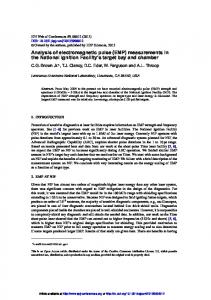
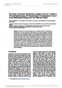
One-dimensional slab models often assume a single volume density of the species and a single gas temperature. The two parameters are then the species column density Nspecies and temperature T . In the most simple case, LTE is assumed. To obtain fluxes, an emitting surface area (radius Re ) must be specified. If we want to deduce profiles in addition to line fluxes, we must assume a ring geometry for the slab, where we need to specify instead of the emitting area the three quantities M∗ (mass of the central star), Rring (radius of the ring), the inclination and the solid angle (Fig. 1). With this, the Keplerian line profile can be calculated. These simple models often ignore effects of the telescope beam, spectral resolution and slit width. 00013-p.2

Summer School „Protoplanetary Disks: Theory and Modeling Meet Observations‰

This approach works reasonably well for lines that originate in regions with small changes in density and temperature, e.g. in some cases the CO ro-vibrational lines, HCN, and water mid-IR lines. It breaks down if lines originate over a wide region of the disk where density and temperature change substantially over the emitting region and especially if different excitation lines originate from different radial regions (changing emitting areas), e.g. the CO pure rotational lines (mm to far-IR wavelengths). As a crude (LTE) approximation, the typical line emitting region can be estimated using the lines upper level energies, e.g. lines with Eupper = 100 K and 300 K may only partially overlap in their emitting region (see Fig. 2 right).

Figure 1: Left: 1D slab geometry. Middle: 1D ring geometry. Right: 2D slab geometry with example profile.

2.2 2D slab models

Often, the gas temperature and the density are not constant. One example are the CO ro-vibrational lines in HD100546. Even though the profiles of the various ro-vibrational bands are the same (Hein Bertelsen et al. 2014), the lines originate in a radially extended region (Brittain et al. 2009). The outer radius of the emission is difficult to constrain and ranges from 50 AU (Goto et al. 2012) to 100 AU (Brittain et al. 2009). In such cases, 2D slab models have been introduced, where the density and temperature are parametrized as radial power laws (Fig. 1, right). In that case, there are two more free parameters, namely the power law index of the density and temperature power law. Instead of a prescribed column density, the volume density n0 at the inner radius Rin is now a free parameter and the same is true for the gas temperature T 0 at the inner radius. The volume density is important in models that take into account non-LTE effects such as UV fluorescence. The higher the volume densities of the collision partner, the less efficient the fluorescent pumping (Thi et al. 2013), because collisions drive the level populations toward LTE. Fitting now the line profiles of high and low excitation ro-vibrational lines allows to determine the radial temperature profile. An example for applying this technique including non-LTE can be found in Brittain et al. (2009). 2.3 Disk models with parametrized chemistry

Many flavors of this model category exists and we describe in the following only three examples. In the model by Piétu et al. (2007), each species is described by its own power law of column density and gas temperature. The scale height of the gas is also parametrized as a power law. The non-LTE 00013-p.3

EPJ Web of Conferences

level populations are calculated using a 2D Monte Carlo line radiative transfer code. Subsequent ray tracing is used to turn the disk models into line emission images which can be compared with interferometric data. In this way, the spatial distribution and abundances of various species can be studied independently. No attempt is made to keep the underlying disk model consistent in terms of temperature, chemical composition and radial extent. A similar approach using parametrized surface density and temperature profiles is used by Williams & Best (2014). Here, the vertical temperature gradient is prescribed by a function connecting the power law midplane and atmospheric temperatures. The CO abundance is parametrized as  −4 n(CO) if T > 20 K and N(H2 ) > 1.3 1021 cm−2 10 (CO) = = 0 if T < 20 K n(H2 ) thus including effects of photodissociation and freeze-out. The authors then use a 3D line radiative transfer code, RADMC-3D, to investigate how the CO submm lines of all three isotopes, 12 CO, 13 CO and C18 O can be used to estimate the disk gas mass. 2D continuum radiative transfer disk models also often assume a parametrized chemistry (fixed species abundances) and T gas = T dust . Here, the dust temperature is calculated self-consistently with the disk radial and vertical structure. In de Gregorio-Monsalvo et al. (2013), the molecular line emission of CO is calculated from an MCFOST model (Pinte et al. 2009, 2006) assuming a constant gas-to-dust mass ratio of 100 and a step function CO abundance: 10−4 with respect to H2 for T dust ≥ 20 K and zero for T dust < 20 K . They find a good match between the disk model of HD 163296 and the ALMA data if the gas temperature inside 80 AU is assumed to be 1.5 T dust , i.e. δT = 0.5 T dust . 2.4 Disk models with parametrized/simple chemistry and Tgas

The last example naturally leads to models in which gas and dust temperature are allowed to decouple. Several studies have shown that gas and dust temperatures de-couple in the surface layers of disks (above AV ∼ 1), where many of the emission lines originate (Jonkheid et al. 2004; Kamp & Dullemond 2004). Since evaluating the detailed heating/cooling balance (see chapter by Woitke 2015) is tedious and computationally expensive, one can approximate this effect by prescribing the gas temperature excess through a simple function T gas = T dust + δT e−r/50 AU .

(1)

There is an additional reason for introducing gas/dust thermal de-coupling: If detailed radiative transfer is considered including dust and line opacities, the assumption of T gas = T dust would produce almost no emission lines if the continuum is optically thick, for example in the near-IR and mid-IR. Emission lines can only emerge in the spectrum if the local line source function is larger than the continuum source function, i.e. the temperature of the gas in the emitting region is higher than the local temperature of the dust. In addition, instead to solving chemical networks to compute the chemistry in the disk (see chapter by Thi 2015), the chemistry can be parametrized as well using e.g. simple step functions in the presence of radial structure and/or snow lines (e.g. Zhang et al. 2013) ⎧ ⎪ if r < 4 AU  ⎪ ⎪ ⎨ inner  if 4 AU≤ r ≤ rsnow H2 O = ⎪ (2) ring ⎪ ⎪ ⎩  if r > r outer

snow

Such models have been invoked by Zhang et al. (2013) to study the water emission over a large wavelength range — from the mid-IR to the sub-mm — and investigate if the location of the snow line and possibly its radial extent (‘slush zone’) can be indirectly deduced from such a dataset. 00013-p.4

Summer School „Protoplanetary Disks: Theory and Modeling Meet Observations‰

Building up model complexity further, the simple step function in chemical profiles can be replaced by very simple chemical models. Meijerink et al. (2009) consider only two processes for the determination of the water vapor/ice equilibrium: Adsorption on cold dust grains and thermal desorption. In addition they reduce the water vapor abundance at gas temperatures above 2000 K using a scaling relation with the ionization parameter ζ/nH (X-rays only) based on the 1D chemical models of Glassgold et al. (2009). Such simplifications of disk chemistry in general should be based on extensive studies involving larger chemical networks to identify the main formation/destruction processes of an individual species and also the parameter space (range of densities, temperatures, radiation fields etc.) where they are valid. The study of Meijerink et al. (2009) has shown that both aspects, the detailed chemistry and the gas/dust thermal coupling, are key for the formation of the mid-IR water lines in the disk surfaces. 2.5 Thermo-chemical disk models

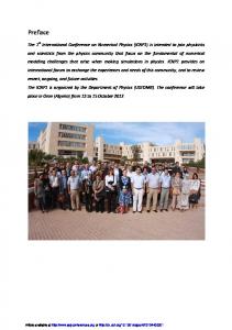
Thermo-chemical disk modeling started in 2004 with the work of Kamp & Dullemond (2004) and Jonkheid et al. (2004), who for the first time included an iterative solution of the gas heating/cooling balance and chemistry into 1+1D disk models. Earlier studies had investigated already the chemistry in disks (starting with Aikawa et al. 1996), and the effects of 2D radiative transfer for FUV and Lyman α (Bergin et al. 2003; Van Zadelhoff et al. 2003) on the disk chemistry. The most complex disk models to date consider the 2D disk structure and solve both for the dust temperature using continuum RT and the gas temperature using an iteration between the heating/cooling balance and the gas chemistry. The gas temperature can then be used further to iteratively solve for the vertical hydrostatic equilibrium. Figure 2 (left) shows the global iteration scheme of such a complex code, ProDiMo (Woitke et al. 2009). Other similar codes — with sometimes more or less complexity — have been published by e.g. Nomura & Millar (2005), Gorti & Hollenbach (2008), and Bruderer et al. (2009). The complexity of such models comes at a price. The computational effort is large compared to much simpler parametrized disk models and an exploration of the full parameter space when matching specific observations is currently beyond reach. In addition, the interplay between dust and gas processes, between chemistry and thermal balance and between physical/chemical processes and radiative transfer poses a challenge in the interpretation of the results. At a much deeper level, the uncertainties in the chemical rates, collisional rates, the simplification of a number of processes (e.g. H2 formation, X-ray ionization, cosmic ray heating) and the possible incompleteness of chemical networks and the heating/cooling processes are ’hidden’ uncertainties in the modeling process. Several of these caveats of course also apply to simpler models. For example, any model calculating non-LTE line emission will suffer from incomplete collisional cross sections and/or missing collision partners. The possibilities that thermo-chemical codes offer are immense and the following list is only meant to give a few diverse examples. Thermo-chemical disk models • enable the simultaneous study of different chemical species within a single model • allow for multi-wavelength studies of combined dust and line emission • are excellent astrochemical laboratories to study and disentangle physical, chemical and radiative transfer processes. An example of a multi-wavelength study of an individual object is HD 163296 (Tilling et al. 2012). The authors provide a single disk model that fits simultaneously the SED, 1.3 mm continuum maps (SMA), the line fluxes of [Oi] 63 μm (Herschel/PACS), 12 CO J=3-2, 2-1 and 13 CO J=1-0 (collected ground-based data), as well as the H2 S(1) (VLT/VISIR) and several far-IR line flux upper limits 00013-p.5

EPJ Web of Conferences

(Herschel/PACS). In addition, the CO J=3-2 spatial emission (SMA) is matched. The data is consistent with a gas-to-dust ratio between ∼ 10 and 100. The flaring index β of the disk surface is most likely below 1.1, meaning that the disk is far from maximum flaring, the 9/7 following from the Chiang & Goldreich (1997) two-layer models for passive disks. Such a disk model provides an excellent starting point for adding in new data that becomes available such as ALMA continuum and line maps, water line observations (Herschel/PACS/HIFI) and additional thermal emission images at shorter wavelengths. It can also be used to guide and help preparing new observing proposals for this target or similar ones.

3 Line fluxes After having discussed the various types of disk models in order of increasing complexity, I turn to the application of these models to actual observational data. The data will be discussed in order of increasing complexity/amount of information starting with the simplest case, in which only line fluxes are available, but the emitting regions remains spatially and spectrally unresolved. 3.1 Vertical temperature gradients

Disk models predict a vertical temperature gradient, decreasing from the upper layers towards the midplane. Van Zadelhoff et al. (2001) showed the resulting layering of gas emission lines: the emission lines of 12 CO J=3-2, 2-1 and 1-0 originate increasingly closer to the midplane. The excitation temperature of their respective upper levels decrease from 33.19 to 5.53 K. Hence, the optimum excitation conditions (maximum contribution to the total line flux) are reached at lower and lower disk heights above the midplane. All of these lines are optically thick in gas-rich primordial disks. However, the isotopologue ratio of 12 CO/13 CO is ∼ 70. Hence, for the same rotational levels, lines of the

Figure 2: Left: Global iteration scheme for a thermo-chemical disk code (ProDiMo, from Woitke c ESO). Right: Radial and vertical layering of the emitting et al. 2009, reproduced with permission region of CO rotational lines in a model for the outer disk around Herbig Ae star HD 100546 (from van der Wiel et al. 2014, reproduced by permission of Oxford University Press).

00013-p.6

Summer School „Protoplanetary Disks: Theory and Modeling Meet Observations‰

rarer isotopologue originate deeper in the disk compared to the main isotopologue. With an isotoplogue ratio of 550, lines of C18 O will originate even closer to the midplane. In the cold outer disk regions of T Tauri disks, the line emission is eventually limited by the CO ice formation. Depending on the radial extent, disks around Herbig stars could stay warm enough to keep CO in the gas phase up to the disk outer radius. Figure 2 (right) shows the layered line emission from a Herbig disk (ProDiMo model). Piétu et al. (2007) used a series of three CO rotational lines from a couple of disks around T Tauri and Herbig stars, to show that the gas temperatures at 100 AU deduced from those lines are consistent with a temperature decrease from 12 CO J=2-1 via 13 CO J=2-1 to 13 CO J=1-0. ALMA will provide such datasets for many more disks and allow a systematic study of the vertical gas temperature gradients in the outer disk. 3.2 Line optical depth

Isotopologues can also be used to assess the optical depth in an emission line. In the optically thin case, if both lines are co-spatial, the line flux ratio should reflect the ratio of the isotopologues. However, the 13 CO/12 CO line ratio is often larger than the isotopic ratio of 1/77, thus indicating that the 12 CO lines are optically thick. The intensity of an emission line, after background subtraction, can be calculated from the difference between the line source function S ν and the background intensity I0 as   Iν = (S ν − I0 ) 1 − e−τν ,

(3)

where τν is the line optical depth. In the Rayleigh-Jeans limit, i.e. at millimeter wavelengths, intensities are measured in temperature units according to T A∗ = Iν

c2 , 2ν2 k

(4)

where ν is the freqency and T A∗ is the observed (beam-filling) line intensity. If the source function and the background radiation field are Planck functions, S ν = Bν (T ex ) and I0 = Bν (T CMB ), with line excitation temperature T ex and cosmic microwave background temperature T CMB = 2.725 K, respectively, we can rewrite Eq. (3) as

  1 1 T A∗ = T 0 1 − e−τν , (5) − exp(T 0 /T ex ) − 1 exp(T 0 /T CMB ) − 1 where T 0 is defined as hν/k. An optically thick line that fills the beam can hence be used to directly measure the line excitation temperature T ex =

T0 ⎛ ⎞ K. ⎜⎜⎜ ⎟⎟ T 0 ⎜   ⎟⎟⎟⎟⎠ ln ⎜⎜⎝1 + ∗ T A + T 0 / exp(T 0 /T CMB ) − 1

(6)

If the excitation temperatures of 13 CO and 12 CO are the same, the 12 CO line is optically thick, and T ex T CMB , we can work out a simple expression that estimates the optical depth τ13 of the 13 CO line from   T A∗ (13 CO) ≈ T A∗ (12 CO) 1 − e−τ13 (7) 00013-p.7

EPJ Web of Conferences

and find

⎞−1 ⎛ T ∗ (13 CO) ⎟⎟⎟ ⎜⎜ ⎟⎠ . τ13 ≈ ln ⎜⎜⎝1 − A∗ 12 T A ( CO)

(8)

Due to its extremely low abundance with respect to the main isotope (factor ∼ 560), C18 O is often used as a column density or mass tracer. If the abundance with respect to H2 is constant and known, its column density can be used to estimate the total cold gas mass. The unknown here is the amount of CO frozen out in the form of ices. 3.3 Thermometers

Molecular line flux ratios can also be used as thermometers. One such example is ammonia, NH3 . As a symmetric rotator, it has next to the rotational quantum number J, which describes the total angular momentum, also a quantum number K associated with the rotation around the principal molecular axis (see chapter by Dionatos 2015). Between the various K-ladders, the dipole selection rules (ΔJ=0, ± 1, ΔK=0) allow only collisional coupling. Hence, at low temperatures, most of the ammonia will be found in the metastable levels J = K. Details on ammonia and its use as a thermometer can be found in Ho & Townes (1983) and Walmsley & Ungerechts (1983). We can thus write down the equations of statistical equilibrium for the lowest levels (1,1), (2,2), and (2,1). With C12 , C21 and C23 being the collisional rates for transitions (1,1)→(2,2), (2,2)→(1,1) and (2,2)→(2,1), respectively, the populations n2 and n1 of levels (2,2) and (1,1) are governed by n2 (C21 + C23 ) = n1C12 .

(9)

Replacing C12 by C21 g1 /g2 exp (−ΔE/T gas ) and introducing the line excitation temperature T 12 between levels (2,2) and (1,1)

n2 g2 ΔE , (10) = exp − n1 g1 T 12 we obtain

T gas

T 12 = 

1+

T gas ΔE

.

ln (1 + C23 /C21 )

(11)

Here, ΔE = hν21 /k ∼ 41 K is the energy difference between levels (1,1) and (2,2), and T gas is the kinetic temperature of the gas. This equation shows that, at low temperatures, T 12 ≈ T gas . Hence, in cold environments, we can use the observable line excitation temperature T 12 as a measure of the physical gas temperature. 3.4 Temperature and density diagnostics

In molecular clouds, line ratios of optically thick low excitation rotational transitions are good probes of gas temperature and density. For such lines, the level populations are dominated by collisions. Collisional rates depend on the volume density of the collision partner and the gas temperature. In the case of CO, where the low rotational lines are thermalized, optically thick and fill the beam, the beam averaged gas temperature can be measured by a single line. Evans (1999) provides an extensive overview of the diagnostic value of a large number of molecular transitions. However, while molecular clouds can be to some extent approximated with either constant density, temperature or at least simple 1D profiles of those quantities, disks are 2D structures. The line emission of different lines is rarely co-spatial and hence many diagnostics appropriate for molecular clouds have to be carefully revisited using 2D thermo-chemical disk models. 00013-p.8

Summer School „Protoplanetary Disks: Theory and Modeling Meet Observations‰ 3.5 Ionization diagnostics

Molecular ions such as HCO+ and N2 H+ depend on the local ionization fraction in the disk, i.e. the electron density. Their abundances are largely determined by the balance of the formation via CO/N2 and H+3 and dissociative recombinations with electrons. If the H2 ionization rate is known, and the column densities of these species can be inferred from the line fluxes, the electron density can be estimated using the column density ratio (Qi et al. 2003). A lower limit to the electron abundance derived for the disk around LkCa15 is 10−8 (Qi et al. 2003). The simple chemistry changes once metals are included such as Fe, Si, Mg. These metals can be easily ionized even deep in the disk (e.g. by secondary UV photons) and provide a significant contribution to the electron abundance, thus leading to a higher ionization fraction. The sources of ionization can be very different ranging from cosmic rays to X-rays and UV radiation. 3.6 Excitation mechanism diagnostics

Ro-vibrational lines of molecules such as H2 and CO can be used to infer the dominant excitation mechanism. Carmona et al. (2011) provide the line ratios of the ro-vibrational lines 1-0 S(0)/1-0 S(1) and 2-1 S(1)/1-0 S(1) in the presence of a variety of excitation mechanisms: LTE, shocks, fluorescence and fluorescence+thermal excitation. The combination of both ratios from observations can be used to exclude some of the excitation mechanisms. Similarly, Brittain et al. (2007) demonstrate that the vibrational temperature derived from near-IR CO ro-vibrational observations can be used to infer the presence of the fluorescent excitation mechanism. The presence of the UV pumping/fluorescence mechanism for CO has been observed directly using HST/COS spectra covering the Fourth Positive band system (A1 Π-X1 Σ+ , 1270-1720 Å) by France et al. (2011).

4 Boltzman diagrams If an entire rotational ladder or several ro-vibrational bands are observed from a single object, we can draw a Boltzman diagram. This diagnostic diagram shows the line flux versus the excitation energy or upper level quantum number. The following derivation is for diatomic molecules. With splitting the energy of a ro-vibrational transition ΔEvJ = ΔEv + ΔE J the population of the ro-vibrational levels can be calculated from



nvJ gJ ΔEv ΔE J gv , exp − exp − = n Zvib kT vib Zrot kT rot

(12)

(13)

where T rot and T vib are the rotational and vibrational excitation temperatures, n is the total particle volume density of the molecule, nvJ the density of the level with the vibrational and rotational quantum numbers (v, J). ΔE J = EvJ − Ev 0 is the energy difference with respect to the rotational ground level of the vibrationally excited level v and ΔEv = Ev − E0 is the energy difference with respect to the ground vibrational state. g J = 2J + 1 and gv = 1 are the statistical weights (vibrational levels in diatomic molecules are non-degenerate). Zrot and Zvib are the rotational and vibrational partition functions. The total population in a vibrational state can be written as

nv ΔEv gv . (14) exp − = n Zvib kT vib 00013-p.9

EPJ Web of Conferences

With this, the population in a specific (v, J) state becomes

nv nvJ ΔE J . = exp − gJ Zrot (T rot ) kT rot

(15)

In the case of LTE and optically thin emission, this can be vertically integrated and provides an expression for the column density NvJ of the level (v, J)

Nv NvJ ΔE J . (16) = exp − gJ Zrot (T rot ) kT rot  Nv = J NvJ is here the total column density in the vibrationally excited state v. The rotational partition function Zrot can be approximated for kT > hB0 by means of rewriting as an exponential integral and substitution u = J(J + 1) (Goldsmith & Langer 1999)



∞ ∞  ΔE J Brot J(J + 1) Zrot = = (17) (2J + 1) exp − (2J + 1) exp − kT rot kT rot J=0 0

 ∞ T rot Brot u du = exp − . ≈ kT rot Brot 0 Molecular rotational constants Brot = hB0 (see chapter by Dionatos 2015) and spectral data for diatomic molecules can be found for example in the NIST database. Energy levels and transitions for the rotational spectroscopy of many molecules (also beyond diatomic) are compiled in the LAMDA database (Schöier et al. 2005). If all lines are optically thin, the ratio NvJ /g J can be calculated from the observed line flux FvJ as NvJ 4π FvJ = , gJ g J hνvJ AvJ Ω

(18)

where Ω is the solid angle of the line emitting region. It is generally assumed that all lines are emitted from the same solid angle. Combining Eq.(16) and Eq.(18) leads to the following expression

4π FvJ Nv ΔE J = exp − . (19) Zrot (T rot ) kT rot g J hνvJ AvJ Ω If the rotational states of the vibrationally excited state are populated according to LTE with rotational excitation temperature T rot as assumed above, we can create a diagram with the natural logarithm of the right hand side versus the excitation energy of the upper level



ΔE J Zrot (T rot ) 4πFvJ . (20) − + ln = ln kT rot g J hνvJ AvJ Nv Ω The second term on the right hand side is an arbitrary constant (unless the column density and emit  ting area are known). In a diagram with x = ΔE J /k and y = ln FvJ /(g J hνvJ AvJ ) , see Fig. 3, we hence expect a line with slope −1/T rot . The rotational temperature found in this way corresponds not necessarily to the gas temperature. The equality T rot = T gas only holds for optically thin LTE emission where all lines are emitted from the same solid angle. For optically thick emission, a correction factor has to be added (Goldsmith & Langer 1999) NvJ = NvJ,thin

τ , 1 − e−τ

00013-p.10

(21)

Summer School „Protoplanetary Disks: Theory and Modeling Meet Observations‰

0 -1

55

Tgas=20, 50, 100, 200, 500 K, Δv=0.1 km/s N=1019 cm-2 log ε(CO)=10-4 log n=8.5

50 ln (FJ/(gJAJhνJ))

1

τline

-2 -3 -4 -5

slope -1/Trot log n=8.5 N=1017...1021 cm-2 log ε(CO)=10-4 Tgas=50 K, Δv=0.1 km/s

45 40 35 30 25

-6

20 500

1000 Eu (K)

1500

2000

500

1000 Eu (K)

1500

2000

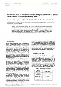
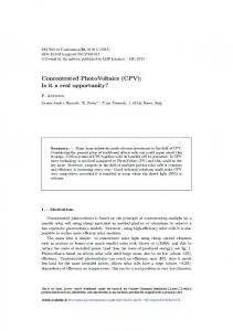
Figure 3: Left: Optical depth as a function of upper level energy Eu for a slab of CO gas with different temperatures. Right: Boltzmann diagram for CO for a slab of constant temperature with varying column density. The solid line indicates the slope of 50 K.

where NvJ,thin is the total emitting column density in the optically thin limit and τ the line optical depth. The latter depends on the assumed line broadening parameter b. The use of Boltzman diagrams is widespread not only in the study of galactic and extragalactic star formation, but also in the analysis of protoplanetary disks. The interpretation of the resulting column densities and temperatures requires a deeper understanding of the SE and radiative transfer. A seminal paper to understand such diagrams and their interpretation is Goldsmith & Langer (1999). Before going into details, it is important to realize that various ways of generating Boltzman diagrams exist in the literature. The x-axis can be energy in Kelvin or any other unit, but also simply the rotational quantum number. In the case of vibrational diagrams, the energies can be absolute values or rotational energies relative to the ground vibrational state. The y-axis can be on a log- or ln-scale. Also some authors include a solid angle while others do not. That can change the scaling by many tens of orders of magnitude. In any case, the absolute y-axis scale is arbitrary and not fixed through line flux observations. 4.1 Optical depth effects

For pure rotational lines of linear molecules, such as CO, the Einstein A coefficient scales as A J,J−1 =

64π4 ν3 μ2 J , 3hc3 2J + 1

(22)

where μ is the permanent electric dipole moment. This means that the Einstein A coefficient increases with J through the last term, but also through the transition frequency ν, which also scales with J. For CO, we find that ν = ΔE/h = 2B0 J, where B0 is the rotational constant (note that the rotational constant is given in different units in the literature and hence the use of different symbols, e.g. B0 , Brot ). The optical depth of the line J → J − 1 can be calculated from τ J,J−1 =

 N J  hν/kTex c3 e A J,J−1 −1 , 3 Δv 8πν

(23)

where N J is the column density of the upper level of the line and Δv the broadening parameter (FWHM in velocity units). Figure 3 (left) shows how the optical depth of the different J lines varies as a function of temperature. The gas temperature determines the distribution over the level populations, 00013-p.11

EPJ Web of Conferences

hence, the level at which the population is maximum. The line optical depth and hence also the line flux depend both on the level population and the Einstein A coefficient. For a sample molecule at fixed temperature, the optical depth depends on the total column density of the molecule (Fig. 3, right). In the optically thin regime log NH ≤ 1019 , measuring the slope (as indicated by the solid line) retrieves the 50 K gas temperature put into the model. For larger column densities, there is a clear upward curvature at low J and fitting a straight line is impossible. However, at higher J where the lines become optically thin even at high column densities, we can measure a rotational temperature from the observational data and and thus obtain a direct estimate of T gas . However, observing such high J rotational lines is more difficult, mostly because of their faintness and observability from the ground. In the literature, two temperature fits are often used in case of rotational diagrams that show curvature, e.g. Meeus et al. (2013). The meaning of these two temperatures with respect to T gas as noted by the authors is often limited, especially in case of protoplanetary disks, and care must be taken not to overinterpret the results (see Sturm et al. 2010). In disk models, very high J values are often required for CO to reach the optically thin line limit. Only then and only if the lines are excited under LTE conditions, the T rot fitted to the high J lines (beyond J = 40) will provide a reasonable estimate of T gas (Thi et al. 2013). The simple two temperatures from slab models could however serve as a valuable means to compare emission properties within a sample of protoplanetary disks. 4.2 LTE versus non-LTE

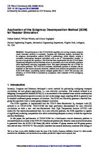
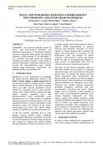
The second effect that can cause a curvature in the Boltzmann diagram is non-LTE. In the chapter by Kamp (2015) it has been shown that deviations from LTE are expected when the densities in the gas are too low to ensure full collisional coupling between the levels. Figure 4 (left) shows a Boltzmann diagram for a slab of CO at 50 K, where the density of the collision partner nH is varied over 5 orders of magnitude. The total CO column is chosen so that all lines are optically thin. At very high densities of the collision partner, the diagram shows a straight line; the level populations are in LTE for log nH = 8.5. As the collision partner density drops below 106.5 cm−3 , a downward curvature starts to appear, again preventing us from fitting a straight line to determine the rotational temperature. The additional complication in an observational diagram is that often non-LTE and optical depth effects are both present simultaneously. 4.3 Application to disks

In protoplanetary disk research, Boltzmann diagrams come with important caveats that often limit their use to certain types of transitions and/or wavelength ranges. Najita et al. (2003) discuss this for the example of CO ro-vibrational lines originating from the inner disks around T Tauri stars. Neufeld (2012) noted that the shape/slope of Boltzmann plots for models with continuous gas temperature distributions can strongly deviate from the single temperature models. One of the most important limitations of pure rotational diagrams is that the lines can originate in very different radial regions of the disk — with large temperature and density gradients and varying solid angle —, turning any slope measurement into a mere theoretical exercise without leading to the determination of a physical quantity. However, for a comparison between different targets that share e.g. the same SED and/or spectral type classification, comparing those ‘theoretical’ slopes can still help the analysis. It is almost obsolete to state that the column densities and rotational temperatures determined using simple slab models (taking optical depth and non-LTE into account) will be meaningless for this case. However, such data can be compared to thermo-chemical disk models. Nice examples of such studies are Bruderer et al. (2012) and van der Wiel et al. (2014). These authors 00013-p.12

Summer School „Protoplanetary Disks: Theory and Modeling Meet Observations‰ 55

R-branch slope -1/Trot

P-branch

0 log n=8.5...4.5 N=1019 cm-2 log ε(CO)=10-4 Tgas=50 K, Δv=0.1 km/s

45 40

log (FJ)

ln (FJ/(gJAJhνJ))

50

35

-2

-4 30 25

v=1-0 P4

-6

v=1-0 P36

20 500

1000 Eu (K)

1500

2000

4.4

4.6

4.8 λ (μm)

5.0

5.2

Figure 4: Left: Boltzmann diagram for CO for an optically thin slab of constant temperaturerm with varying collision partner density nH . The solid line indicates the slope of 50 K. Right: non-LTE Flux versus wavelength from a slab model with T gas = 800 K and column densities ranging from NH = 1019 to 1023 cm−2 for the fundamental CO ro-vibrational band (collision partner density log nH = 9.5, log (CO) = −4, Δv = 0.1 km/s). Dashed vertical lines indicate the position of the P4 (J=4-3) and P36 (J=36-35) lines.

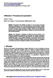
study the CO rotational ladder from combined ground-based and space-based observations in the context of a series of proposed disk structures for the object HD 100546. The data covers upper level J from 3 to 36. The high excitation rotational lines originate in a narrow radial region very close to the inner rim of the outer disk at ∼ 10 AU. On the other hand, the low J submm lines originate between 50 and 300 AU. The comparison of the observed Boltzmann diagram with the modeled one reveals how well the radial gas temperature gradients are captured between 10 and 300 AU. The far-IR wavelength range with access to the J > 10 transitions is crucial for such studies but unaccessible from the ground. Currently, only SOFIA has access with various instruments and resolution to the wavelength region that covers the mid and high J CO lines but its sensitivity is limited. The next possible mission to continue this work for larger samples of protoplanetary disks would be SPICA with its SAFARI instrument. The Japan Aerospace Exploration Agency (JAXA) leeds the proposal for the SPICA mission. It is planned to be a 3 m class cooled (6 K) observatory in space. SAFARI is the medium resolution (R ∼ 3000) far-IR spectrometer (30-210 μm) developed by a European consortium. There are however cases, where the lines do originate over a narrow radial disk region, e.g. rovibrational lines of CO, OH, water. They are usually emitted from the inner disk (inside a few 10 AU) and originate over a narrow radial range (appropriate for their excitation). Ideally this needs to be checked with resolved line profiles. If all profiles show the same shape and FWHM, it can be safely concluded that their radial line forming region is very similar. A good example are the CO ro-vibrational lines in HD 100546 (Brittain et al. 2009; Hein Bertelsen et al. 2014). Figure 4 (right) shows how the CO ro-vibrational line flux from a slab model changes with wavelength across the fundamental 5 μm band. The characteristic R- and P-branch signature is clearly visible for low optical depth. However, at large optical depth, low and high J lines differ only by a factor of a few. Even if the lines originate from the same radial disk region, still some or all lines could show non-LTE and optical depth effects. If the line coverage with J is sparse or has larger gaps, the column densities and temperatures derived with simple slab models will have very large uncertainties. More importantly, it becomes difficult to compare the temperatures derived from different observational sets with different J coverage (Fig. 5). Another problem when comparing different datasets is the absolute flux calibration. Slit loss effects will depend on the seeing, the performance of an adaptive optics 00013-p.13

EPJ Web of Conferences

(AO) system and the centering and position angle (PA) of the slit. Many of these effects are discussed in detail in Hein Bertelsen et al. (2014).

5 Line profiles The previous section already alluded to the additional information gained through lines profiles: We have a handle on the spatial origin of the emission even if the observation itself is spatially unresolved. The line profile contains kinematic information — unaccessible through dust observations — and thus indirect information on the spatial distribution of the emission. The following subsections will discuss the various kinematic signatures detected in disks (rotation, winds and outflows) and some issues we need to be aware of when interpreting line profiles: Blending, turbulence and instrumental effects. 5.1 Keplerian profiles

Figure 6 shows the velocity pattern and the resulting line profile from a disk in Keplerian rotation viewed edge-on around the central star. The high velocities, i.e. the wings of the line profile are dominated by the inner disk which contains less surface area. The lowest velocities correspond to the outer disk. The dip around the central velocity is caused by the disks finite outer radius, i.e. the lowest velocity bins do not show closed loops and hence lack emitting surface area. Beckwith & Sargent (1993) investigated in their seminal paper the line emission from disks and the diagnostic power in detail. If the line emission is optically thick and the disk emission had a sharp outer edge, we could measure that outermost emitting radius simply from the peak separation. The peaks occur at the projected Keplerian velocities ± vout sin i with i being the inclination of the disk with respect to the observer (i = 0 is face-on) and vout the velocity at the outer edge of the emitting area. Similarly, the full width at zero intensity (FWZI) provides an upper limit for the innermost radii contributing to the line emission. Due to the noise in the continuum, small contributions from gas inward of the inner radius cannot be ruled out. For the specific object discussed already in the case of line fluxes, HD 100546, the line profiles of low and intermediate pure rotational lines have been observed with ground-based (APEX) and

Figure 5: Rotational temperatures derived from non-LTE slab models including optical depth based on the full sample of fundamental ro-vibrational lines and various selected line samples from a model of the protoplanetary disk around the Herbig Ae star HD 163296. The grey shaded area outlines all possible solutions, the red lines the best fit. Temperatures and column densities refer to the best fit (figure courtesy of Rosina Hein Bertelsen).

00013-p.14

Summer School „Protoplanetary Disks: Theory and Modeling Meet Observations‰

Figure 6: Left: Velocity contours in a disk around a two solar mass star with an inclination angle i = 60◦ . The colored areas indicate velocity intervals around v = −10.0, −5.0, −3.6, −2.6, −1.0, 0, 1.0, 2.6, 3.6, 5.0 and 10.0 km/s with a width of 0.2 km/s. Right: Resulting line profile with the same colored velocity bins on top (figure courtesy of Andres Carmona).

16−15

10−9

3−2

1.2 T MB [K] (normalized)

1.0 0.8 0.6 0.4 0.2 0.0 −0.2 −5

0

5

10

15

−5

0

5 10 −1 V LSR [km s ]

15

−5

0

5

10

15

Figure 7: CO line profiles from the disk around HD 100546; J levels for line identification are shown on the top. Figure courtesy of Davide Fedele, for details see Fedele et al. (2013).

space-based (Herschel/HIFI) instruments (Fedele et al. 2013). At a distance of 97 pc (HD 100546), the disk emission is not spatially resolved (beam sizes ranging between 11" and 19"). The FWHM and peak separation increase clearly with J (Fig. 7). So now, besides the fluxes, we can also use the peak separation and FWHM to derive the radial disk structure. Models that can fit the Boltzman diagram may not fit at the same time the change in line profile with J. Hence, line profiles are crucial to break modeling degeneracies that keep existing if only unresolved data is used. 00013-p.15

EPJ Web of Conferences 5.2 Winds and outflows

Besides disk kinematics, line profiles can disentangle the origin of the emission: disk, disk wind, jet, outflow. Lines that lend themselves to studies of disk winds are for example the fine structure lines of Ne and Ar in the mid-IR which originate clearly in the hot ionized gas of the inner disk surface. Also mid-IR rotational lines of H2 should originate from the inner disk, but detection has proven difficult (Carmona et al. 2008). Jets are in general associated with much higher velocities and higher collimation than outflows and disk winds. Examples of line profiles likely originating from a jet and shifted by more than 100 km/s can be found in Baldovin-Saavedra et al. (2012) (see Fig. 8a). Photoevaporative winds should imply velocities of the order of a few km/s (for a recent review, see Alexander et al. 2014) and thus require not only high spectral resolution, but also an accurate independent measurement of the stellar radial velocity for their detection (figure 5 of Alexander et al. 2014). Nevertheless, line profiles can be quite complex even in the case of pure disk emission. The radial flux distribution in a disk can be more complex than a simple power law. In some cases, the inner rim could be vertically extended and thus provide a large contribution to the line profile. One such case is shown in Fig. 8c: The [Ne ii] line from a FUV and X-ray irradiated hydrostatic disk model (Aresu et al. 2012). The disk model shows a strong puffed up inner rim and a secondary puffed-up region that is radially more extended. In such cases, line profiles can display multiple peaks. Depending on the S/N and telluric contamination, such line profiles can be detected in real disks. Two interesting examples are the CO ro-vibrational lines and [O i] 6300 Å line profile of HD 101412 (Fig. 8b) and the [Ne ii] 12.81 μm line from GM Aur (figure 5 of Najita et al. 2009). Also, near-IR H2 lines have been used to study the temperature and kinematics of shocked gas in jets/outflows around young stars (for a recent review of observations of jets/outflows, see Bally et al. 2007). 5.3 Line blending

The resolution of spectrographs varies from a few hundred (gratings, Fourier Transform Spectrometer) to ∼ 106 (echelle and heterodyne). The highest spectral resolution for the Infrared Spectrograph onboard Spitzer was 600. At such low resolution, mid-IR rotational and ro-vibrational lines from various molecules, but even from the same molecule, are heavily blended. Hence, instead of individual line fluxes, only fluxes for an entire complex/blend can be extracted (see Fig. 9, left). We need to distinguish between blending caused by such limited spectral resolution and real physical blending, where lines originating in different parts of a disk (at different radial velocities) can physically interact, e.g. re-absorption of photons within a line. This happens very rarely though and only if the line density is extremely high, e.g. for near-IR ro-vibrational lines and/or lines of different isotopologues (e.g. 12 CO and 13 CO). High spectral resolution instruments beyond optical wavelengths often require more complex data reduction and intricate understanding of the instrument. Then why do it? The reasons are twofold: (1) Line blending is minimized and we can hope to extract individual lines, ideally even resolve their profiles, (2) Lines are smeared out at low resolution, meaning molecules with abundances well below the dominant species CO and water, such as CH4 , C2 H2 , HCN, will disappear in the continuum. On the modeling side, especially in the mid-IR with its very high density of lines, approximate radiative transfer concepts are used to predict spectra for comparison with observations. One such approach is the escape probability method that is discussed in the chapters by Kamp (2015) and Woitke (2015). However, for detailed fitting of wider wavelength ranges such simple schemes have limitations. Figure 9 (right) shows the difference in the modeled spectrum between a simple escape probability method and a detailed full line radiative transfer (FLiTs). 00013-p.16

Summer School „Protoplanetary Disks: Theory and Modeling Meet Observations‰

(b)

(a)

(c)

Figure 8: (a) Montage combining the possible geometry of a disk with jet and wind from Pontoppidan c AAS, reproduced with permission) with a sample of observed [Ne ii] line profiles et al. (2011, from several young stellar objects showing likely disk origin (CoKu Tau), disk+wind origin (V892 c ESO). Tau) and jet origin (MHO-1) (Baldovin-Saavedra et al. 2012, reproduced with permission (b) Overlay of complex line profiles of [O i] 6300 Å, CO ro-vibrational and overtone emission from HD 101412 (reproduced with permission from figure 4.13, PhD thesis of Gerrit van der Plas 2010). (c) Disk emission can also deviate in the absence of winds from a simple Keplerian profile (taken from c ESO). The line emission has a strong figure 6 of Aresu et al. 2012, reproduced with permission high velocity contribution from the inner rim (line shoulders) and a more extended second component (narrow emission peaks).

5.4 Turbulence

In the chapter by Kamp (2015) several line broadening mechanisms have been discussed; the ones most relevant to disks are thermal and turbulent broadening. Turbulence in disks can be caused by instabilities, such as gravitational instability, magneto-rotational instability or hydrodynamic instability (e.g. Balbus & Hawley 1998). However, hydrodynamical and magneto-hydrodynamical (MHD) simulations do not provide conclusive evidence for the mechanism behind and the amount of turbulence to be expected in disks. In a recent study, Simon et al. (2011) used ideal and non-ideal MHD simulations to provide values for turbulent velocities as a function of radial distance and height in the disk. Typical values are of the order of 10-100 % of the sound speed (c s ), while they drop to 1 % of the sound speed in dead zones. However, direct observations of turbulent velocities spatially resolved throughout the disk remain very difficult if not impossible. Several attempts to detect turbulence directly from gas emission line profiles have been made. Hughes et al. (2011) used very high spectral resolution (44 m/s, well below expected value for tur00013-p.17

EPJ Web of Conferences

Figure 9: Left: Mid-IR spectra of water calculated for a range of different spectral resolutions. At the bottom, the Spitzer spectrum of TW Cha is shown for comparison (figure 5 of Pontoppidan et al. c AAS, reproduced with permission). Right: Mid-IR spectrum calculated at R = 600 with 2010, escape probability (black line) and the new detailed fast RT code FLiTs (red line, courtesy of Michiel Min).

bulent velocities) CO J=3-2 line profiles observed with the SMA. In combination with a 1+1D disk model, the best fit to the line profiles suggests for TW Hya a broadening parameter b < 40 m/s (< 0.1 c s ) and for HD 163296 b ∼ 300 m/s (∼ 0.4 c s ). The largest degeneracy is between the thermal and turbulent broadening. If the disk model had a different temperature distribution, this would immediately affect the deduced turbulent broadening parameter. Hence, ideally the physical structure of the disk model should be constrained by one set of spatially resolved gas observations, while the turbulent broadening is then deduced from another. Also, using neutral species will always include the uncertainty of the coupling efficiency between neutral and ionized gas. If the process driving turbulence is MRI, the motions should be best measured in the ionized gas. Guilloteau et al. (2012) attempted to use one line (CS J=3-2) to determine the disk thermal structure and then another one (CS J=5-4) to deduce the turbulent broadening. Because of the higher mass of CS (44 mu ) compared to CO (28 mu ), the thermal velocities will be lower than for CO. In addition, the main isotopologue lines of CS are more optically thin than CO, so that these lines can probe turbulence closer to the midplane. From power law disk models, Guilloteau et al. (2012) deduced turbulent velocities between 50 and 150 m/s (depending on the gas temperature power law profile) at 300 AU in the disk around DM Tau. A remaining problem is that the CS J=3-2 line most likely originates above and outwards of the CS J=5-4 line. Hence the temperature gradient deduced from the former may not directly apply to the latter. ALMA will make a step further by observing many more transitions, thus removing remaining degeneracies between the disk thermal structure and the size of turbulent velocities. 00013-p.18

Summer School „Protoplanetary Disks: Theory and Modeling Meet Observations‰ 5.5 Slit effects

Last but not least, instrumental effects can influence the line fluxes and profiles. The most important example are slit effects. Depending on the physical size of the emitting region and the width of the slit, some of the line flux can be lost. The point spread function (PSF) can be wider than the slit width and even in the presence of an AO system lead to some flux loss. In addition, proper centering of the slit can cause problems especially if the emitting area is of the same order as the slit width. If the disk emission is more extended than the slit, not only flux, but also part of the velocities will be lost. If a slit is aligned with the minor axis of a disk, this can lead to single peaked emission lines instead of double-peaked ones since the wings of the velocity profile will fall outside the slit. In a recent study, Hein Bertelsen et al. (2014) show the CO ro-vibrational line profiles that originate from rotating the VLT/CRIRES slit through various PAs in the presence of possibly inaccurate centering (offsets up to 0.2" with respect to the minor axis of the disk). Figure 10 shows the resulting line shape variations that range from symmetric to asymmetric and from single peaked to doublepeaked.

Figure 10: Line profile variations depending on the position angle of the slit (0o to 175o in steps of 10 degrees). The inner radius of the emitting region and the slit width are of similar size. Offsets with respect to the star along the disk minor axis range from −0.2 to 0.2". The y axis is normalized flux from (−0.1 . . . 1.7), while the x axis ranges from −15 km/s to +15 km/s. Figure from Hein Bertelsen c ESO). et al. (2014, reproduced with permission

00013-p.19

EPJ Web of Conferences 5.6 Spectro-astrometry

If disks are observed with a long slit spectrograph such as VLT/CRIRES and VISIR in the near-IR using AO, the spatial distribution of the emission can be retrieved — even though only in one direction, the slit PA. If enough slit PAs are taken for the same target, even the two-dimensional spatial emission from the disk could be reconstructed. However, such observations are very time consuming and difficult to reduce. The method is described in detail in Whelan & Garcia (2008) and I introduce only some basic quantities and example applications here. Figure 11 illustrates the basic concept. The dispersion direction across the slit denotes wavelength and the direction along the slit denotes spatial distance from the central object. The line clearly shows up around the corresponding rest wavelength, but it has a distinctive s-shape pattern, which originates from Keplerian rotation in a disk. In addition, in this example, the width of the continuum signal is spatially less extended than the signal at the position of the line. We can fit a Gaussian at every wavelength and measure the FWHM and the Spatial Peak Position (SPP) as a function of wavelength. These quantities tell us immediately whether the line emission is spatially resolved and what its kinematic signature is.

Figure 11: Sketch of the main concept of spectroastrometry of a rotating protoplanetary disks; figure inspired by figure 1.11 from the PhD thesis of Gerrit van der Plas (2010). Spectro-astrometry has been used for example to demonstrate the absence/presence of molecular gas in dust cavities. Examples are CO ro-vibrational emission from the inner rim of the outer disk in HD 141569 (Goto et al. 2006), and CO emission from inside the dust cavity for SR21 and HD 135344B (Pontoppidan et al. 2008). All three disks show large gaps in the dust submm continuum images. Spectro-astrometry is the first step towards complete spatially resolved data available from interferometers, which will be discussed in the next section. 00013-p.20

Summer School „Protoplanetary Disks: Theory and Modeling Meet Observations‰

6 Spatially resolved line emission The highest amount of information can be derived from spatially and spectrally resolved lines. Such data is commonly taken by radio, millimeter and sub-mm interferometers such as the VLA, IRAM Plateau de Bure, SMA and ALMA. Interferometric data comes as a data cube (see chapter by Ilee & Greaves 2015) with two spatial dimensions and one spectral dimension. In order to visualize the data, we often use either 1D slices or 2D slices through the cube. Besides looking at the spatially integrated line profile, which we did in the previous section, we can now study moment maps (spatial maps), channel maps (velocity channels) and position-velocity diagrams (along one spatial dimension). An example of such a dataset is shown in Fig. 12. Diagrams of molecular line emission such as the one on the left, where the intensity-weighted velocity map is shown in color, have been used to proof that the extended dust emission around young pre-main sequence stars is due to inclined thin disks in Keplerian rotation (e.g. Mannings & Sargent 1997) and to derive disk inclinations and radial profiles. However, with the exquisite high spatial and spectral resolution of ALMA, position-velocity diagrams become increasingly useful diagnostics. We first have a close look at these key diagnostic diagrams before turning to the disk structure that can be deduced from such datasets (radial and vertical).

Figure 12: Left: Zeroth (contours) and first moment (color) map of the CO J=3-2 line emission from the disk around HD 100546 taken with ALMA. Right: position-velocity diagram for the same observation. Superimposed in red and yellow are the Keplerian velocity curves expected for inclinations of c AAS, reproduced 40 and 30 degrees respectively. Both figures are taken from Pineda et al. (2014, with permission).

6.1 Moment maps

The various moments that can be constructed are: • Zeroth moment — velocity integrated intensity • First moment — intensity weighted velocity • Second moment — intensity weighted velocity dispersion. The higher moment maps depend on the lower moment ones, so the noise level will increase with the order. Figure 12 (left) shows an example for zeroth moment contours displayed on a color map of the first moment. While the intensity contours clearly show the spatial distribution of the emission, the 00013-p.21

EPJ Web of Conferences

FWHM along the various disk axis, the color map displays the typical pattern of Keplerian rotation with one half of the disk turning away from us and the other half towards us. From that color map, the disk minor and major axes become immediately evident (dotted lines). 6.2 p-v diagrams

Position-velocity diagrams are created by defining a spatial cut through the data cube, e.g. along the major disk axis (see Fig. 12, right). If the mass of the central star is known — 2.4 M in this case —, Keplerian velocities can be overplotted for various inclinations. The outermost contours allow then an accurate determination of the disk inclination and the detection of infall/outflow or warps. Pineda et al. (2014) note that the contours inside 2" are better reproduced by an inclination of 30o , while those outwards of 2" agree better with 40o . 6.3 Channel maps

We can also choose to display spatial maps for each velocity slice. For that, we define a small velocity interval over which the intensity is integrated and then displayed as a function of position. An example is given — again for an ALMA dataset — in Fig. 13, showing the CO J=3-2 channel maps for the disk around HD 163296 (de Gregorio-Monsalvo et al. 2013). Due to the high quality of the new ALMA data, several features are now visible in these maps. The usual butterfly pattern resulting from the dipole nature of the Keplerian velocity field appears double. The systemic (heliocentric) velocity of the star itself is 5.79 km/s (Hughes et al. 2011). The more pronounced high intensity butterfly in Fig. 13 comes from the disk surface facing the observer (front surface), while the fainter thin butterfly pattern originates from CO in the rear surface of the disk. The reason for the clear separation between the front and rear disk surface is that the CO emission is very optically thick and arises very high up in the disk close to the surface. In addition, the inclination angle of 45o and the fact that the disk is optically thin in the neighboring continuum are favorable as well. 6.4 Radial and vertical disk structure

Since ALMA has just started to revolutionize the field, this section will not try to summarize the recent findings but rather concentrate on a brief outlook of what will likely be doable over the next decade. Besides what we know ALMA can do, there will always be unexpected discoveries. Line data cubes are very powerful in providing direct information on how the gas is distributed radially and vertically in disks. They open the possibility to measure disk scale heights, flaring angles, and temperature distributions directly. They will be a key tool to detect disk asymmetries and/or warps caused by e.g. planets or instabilities. We expect to measure the ionization fraction as a function of position and assess the role of MRI in driving disk evolution. With the superb kinematic resolution, even low velocity winds and flows will be easily detected and provide direct insight into disk dispersal mechanisms. The measurement of disk scale heights and temperature distributions will test 2/3D radiative transfer models of disks and the assumption of vertical hydrostatic equilibrium. How important are (magneto-)hydrodynamical instabilities is shaping the overall disk structure? How well do we understand the heating/cooling balance of the gas and do we miss important processes? Besides these direct measurements, the data cubes will put thermo-chemical disk models on the spot. Does the chemical structure/layering agree with the observations, e.g. the location of the warm 00013-p.22

Summer School „Protoplanetary Disks: Theory and Modeling Meet Observations‰

Figure 13: Channel maps of the CO J=3-2 emission from the disk around HD 163296 (spectral resolution = 0.21 km/s). The figure is taken from de Gregorio-Monsalvo et al. (2013, reproduced with c ESO). permission

molecular layer, the position of snow and ice lines. How important are radial and vertical mixing processes with respect to simple stationary or time-dependent chemistry? Does the observed chemical composition require varying C/O ratios, strong metal depletion (enhanced condensation/dust formation compared to the ISM)? Do the models miss chemical pathways? How much of the chemical memory of the molecular cloud phase gets preserved? Acknowledgements The research leading to these results has received funding from the European Union Seventh Framework Programme FP7-2011 under grant agreement no 284405. The work benefitted a lot from discussions within the DIANA team. In addition, I would like to thank Silvia Vicente, Andres Carmona and Irina Leonhardt for their valuable comments which greatly improved the manuscript.

References Aikawa, Y., Miyama, S. M., Nakano, T., & Umebayashi, T. 1996, ApJ, 467, 684 00013-p.23

EPJ Web of Conferences

Alexander, R., Pascucci, I., Andrews, S., Armitage, P., & Cieza, L. 2014, Protostars and Planets VI, 475 Aresu, G., Meijerink, R., Kamp, I., et al. 2012, A&A, 547, A69 Balbus, S. A. & Hawley, J. F. 1998, Reviews of Modern Physics, 70, 1 Baldovin-Saavedra, C., Audard, M., Carmona, A., et al. 2012, A&A, 543, A30 Bally, J., Reipurth, B., & Davis, C. J. 2007, Protostars and Planets V, 215 Beckwith, S. V. W. & Sargent, A. I. 1993, ApJ, 402, 280 Bensch, F. 2006, A&A, 448, 1043 Bergin, E., Calvet, N., D’Alessio, P., & Herczeg, G. J. 2003, ApJL, 591, L159 Brittain, S. D., Najita, J. R., & Carr, J. S. 2009, ApJ, 702, 85 Brittain, S. D., Simon, T., Najita, J. R., & Rettig, T. W. 2007, ApJ, 659, 685 Bruderer, S., Doty, S. D., & Benz, A. O. 2009, ApJSS, 183, 179 Bruderer, S., van Dishoeck, E. F., Doty, S. D., & Herczeg, G. J. 2012, A&A, 541, A91 Carmona, A., van den Ancker, M. E., Henning, T., et al. 2008, A&A, 477, 839 Carmona, A., van der Plas, G., van den Ancker, M. E., et al. 2011, A&A, 533, A39 Chiang, E. I. & Goldreich, P. 1997, ApJ, 490, 368 Crockett, N. R., Bergin, E. A., Neill, J. L., et al. 2014, ApJ, 787, 112 de Gregorio-Monsalvo, I., Ménard, F., Dent, W., et al. 2013, A&A, 557, A133 Dionatos, O. 2015, in EPJ Web of Conferences, Vol. 102, Summer School on Protoplanetary Disks: Theory and Modeling Meet Observations, ed. I. Kamp, P. Woitke, & J. D. Ilee Evans, II, N. J. 1999, ARA&A, 37, 311 Fedele, D., Bruderer, S., van Dishoeck, E. F., et al. 2013, ApJL, 776, L3 France, K., Schindhelm, E., Burgh, E. B., et al. 2011, ApJ, 734, 31 Glassgold, A. E., Meijerink, R., & Najita, J. R. 2009, ApJ, 701, 142 Goldsmith, P. F. & Langer, W. D. 1999, ApJ, 517, 209 Gorti, U. & Hollenbach, D. 2008, ApJ, 683, 287 Goto, M., Usuda, T., Dullemond, C. P., et al. 2006, ApJ, 652, 758 Goto, M., van der Plas, G., van den Ancker, M., et al. 2012, A&A, 539, A81 Guilloteau, S., Dutrey, A., Wakelam, V., et al. 2012, A&A, 548, A70 Hein Bertelsen, R. P., Kamp, I., Goto, M., et al. 2014, A&A, 561, A102 00013-p.24

Summer School „Protoplanetary Disks: Theory and Modeling Meet Observations‰

Ho, P. T. P. & Townes, C. H. 1983, ARA&A, 21, 239 Hughes, A. M., Wilner, D. J., Andrews, S. M., Qi, C., & Hogerheijde, M. R. 2011, ApJ, 727, 85 Ilee, J. & Greaves, J. 2015, in EPJ Web of Conferences, Vol. 102, Summer School on Protoplanetary Disks: Theory and Modeling Meet Observations, ed. I. Kamp, P. Woitke, & J. D. Ilee Jonkheid, B., Faas, F. G. A., van Zadelhoff, G.-J., & van Dishoeck, E. F. 2004, A&A, 428, 511 Kamp, I. 2015, in EPJ Web of Conferences, Vol. 102, Summer School on Protoplanetary Disks: Theory and Modeling Meet Observations, ed. I. Kamp, P. Woitke, & J. D. Ilee Kamp, I. & Dullemond, C. P. 2004, ApJ, 615, 991 Mannings, V. & Sargent, A. I. 1997, ApJ, 490, 792 Meeus, G., Salyk, C., Bruderer, S., et al. 2013, A&A, 559, A84 Meijerink, R., Pontoppidan, K. M., Blake, G. A., Poelman, D. R., & Dullemond, C. P. 2009, ApJ, 704, 1471 Najita, J., Carr, J. S., & Mathieu, R. D. 2003, ApJ, 589, 931 Najita, J. R., Doppmann, G. W., Bitner, M. A., et al. 2009, ApJ, 697, 957 Neufeld, D. A. 2012, ApJ, 749, 125 Nomura, H. & Millar, T. J. 2005, A&A, 438, 923 Piétu, V., Dutrey, A., & Guilloteau, S. 2007, A&A, 467, 163 Pineda, J. E., Quanz, S. P., Meru, F., et al. 2014, ApJL, 788, L34 Pinte, C., Harries, T. J., Min, M., et al. 2009, A&A, 498, 967 Pinte, C., Ménard, F., Duchêne, G., & Bastien, P. 2006, A&A, 459, 797 Pontoppidan, K. M., Blake, G. A., & Smette, A. 2011, ApJ, 733, 84 Pontoppidan, K. M., Blake, G. A., van Dishoeck, E. F., et al. 2008, ApJ, 684, 1323 Pontoppidan, K. M., Salyk, C., Blake, G. A., et al. 2010, ApJ, 720, 887 Qi, C., Kessler, J. E., Koerner, D. W., Sargent, A. I., & Blake, G. A. 2003, ApJ, 597, 986 Schöier, F. L., van der Tak, F. F. S., van Dishoeck, E. F., & Black, J. H. 2005, A&A, 432, 369 Simon, J. B., Armitage, P. J., & Beckwith, K. 2011, ApJ, 743, 17 Sturm, B., Bouwman, J., Henning, T., et al. 2010, A&A, 518, L129 Thi, W.-F. 2015, in EPJ Web of Conferences, Vol. 102, Summer School on Protoplanetary Disks: Theory and Modeling Meet Observations, ed. I. Kamp, P. Woitke, & J. D. Ilee Thi, W. F., Kamp, I., Woitke, P., et al. 2013, A&A, 551, A49 Tilling, I., Woitke, P., Meeus, G., et al. 2012, A&A, 538, A20 00013-p.25

EPJ Web of Conferences

van der Wiel, M. H. D., Naylor, D. A., Kamp, I., et al. 2014, MNRAS, 444, 3911 Van Zadelhoff, G.-J., Aikawa, Y., Hogerheijde, M. R., & van Dishoeck, E. F. 2003, A&A, 397, 789 Van Zadelhoff, G.-J., van Dishoeck, E. F., Thi, W.-F., & Blake, G. A. 2001, A&A, 377, 566 Walmsley, C. M. & Ungerechts, H. 1983, A&A, 122, 164 Whelan, E. & Garcia, P. 2008, in Lecture Notes in Physics, Berlin Springer Verlag, Vol. 742, Jets from Young Stars II, ed. F. Bacciotti, L. Testi, & E. Whelan, 123 Williams, J. P. & Best, W. M. J. 2014, ApJ, 788, 59 Woitke, P. 2015, in EPJ Web of Conferences, Vol. 102, Summer School on Protoplanetary Disks: Theory and Modeling Meet Observations, ed. I. Kamp, P. Woitke, & J. D. Ilee Woitke, P., Kamp, I., & Thi, W.-F. 2009, A&A, 501, 383 Zhang, K., Pontoppidan, K. M., Salyk, C., & Blake, G. A. 2013, ApJ, 766, 82

00013-p.26