PPeettrroolleeuum m && C Cooaall IISSN 1337-7027 Available online at www.vurup.sk/pc Petroleum & Coal 48 (2), 15-23, 2006
MODELING AND SIMULATION OF AMMONIA SYNTHESIS REACTOR Ali Dashti, Kayvan Khorsand1, Mehdi Ahmadi Marvast, Madjid Kakavand Research Institute of Petroleum Industry (RIPI), Pazhouheshgah Blvd., Khairabad, Qom Road, Tehran, Iran. 1 corresponding author,
[email protected] Received May 1, 2006; accepted June 24, 2006
Abstract In this paper an industrial ammonia synthesis reactor has been modeled. The reactor under study is of horizontal type. This reactor which is under the license of Kellogg Company is equipped with three axial flow catalyst beds and an internal heat exchanger in accompany with a cooling flow. The achieved modeling is one dimensional and non-homogenous. Considering the sever effect of internal heat exchanger on reactor operation, it has been simulated by calculation of film heat transfer coefficients in its tube and shell and then, taking into account the shell thermal resistance and fouling coefficient, obtaining the overall heat transfer coefficient. So in the developed software, the heat transfer coefficient is first calculated using the conditions of the input flow to the exchanger and then the input flows to the first and second beds are calculated. The differential equations have been solved using Rung Kutta 4 method and the results have been compared with the available industrial data. Finally the capability of the developed software for industrial application has been investigated by changing the reactor operation conditions and studying their effects on reactor output. Key words: ammonia, reactor, modeling, simulation
1. Introduction Ammonia Synthesis is a very important process in chemical complexes. Ammonia is the initial chemical material for a variety of industries. It is used in production of chemical fertilizers, explosive materials, polymers, acids and even coolers. Simulation can play an important role to give an insight of the industrial units and hence simulation of Ammonia unit is very important to help us investigate the different operation modes of this unit and optimize that. Ammonia synthesis loop is the most important part of this unit which better understanding of its bottleneck can led us to make the operation yield higher than before. 2. Ammonia Synthesis Loop In ammonia production unit, the synthesis loop is located after the syngas production and purification units. Ammonia synthesis process takes place in high pressure and hence high power multi cycle compressors are used to supply the required pressure. The Kellogg synthesis reactor incorporated in this loop is of horizontal type with three beds. To control the temperature between first and second beds, an internal heat exchanger has been used in which the input feed to the first bed and the output gas from the same bed have thermal exchange. In addition to the mentioned heat exchanger, the quench gas flow is also used for control of temperature. The input feed to the reactor, is first divided into two parts, before entrance. One part is considered as feed and the other part as quench gas. The feed, after entering the reactor, passes through the empty spaces of the beds as well as the reactor walls and gets slightly heated. When reaching to the end of the reactor, it passes through the shell of the internal heat exchanger and its temperature reaches 400 ºC. Tubes of the heat exchanger contain the output gas from the first bed. Quench gas is used to control the inlet temperature of the first bed. The required temperature for inlet of the first bed is 371 ºC. Output gas,
Ali Dashti et al./Petroleum & Coal 48(2) 15-23 (2006)
16
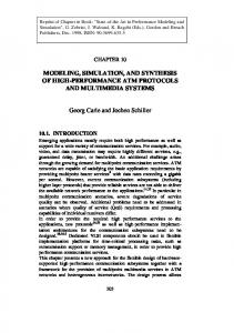
after warming up, is then entered to first catalytic bed. Figure 1 depicts the schematic diagram of a Kellogg horizontal reactor.
Fig.1 Ammonia Synthesis Reactor - Kellogg method [1] When the gas passes the first bed and the reaction is taken place, its temperature increases and reaches 496 ºC. It then enters the tubes of the heat exchanger to cool down. Gas is then entered from top of the second bed. Temperature rises again as the reaction takes place in the second bed. No specific operation is carried out between beds two and three. In fact these two beds act as a single bed whose length is twice the length of each bed. The catalyst of this reactor is magnetic ferro oxide. 3. Mathematical Model By modeling of the synthesis reactor, temperature, concentrations and pressure profiles are obtained. Of course testing of the model based on the above parameters is achieved at the end of each bed as industrial data are not usually available along the length of the bed. The following assumptions have been made for this modeling: 1. One-dimensional Cartesian coordinate has been considered along with the bulk flow. 2. Penetration of mass and heat is ignored, as the fluid velocity is very high in industrial scale. 3. Density is constant 4. Concentration and temperature on catalyst surface and bulk of gas are equal. 5. The effects of penetration resistance in catalyst, temperature gradient and catalyst inside concentration have been incorporated in the equations by a coefficient. [2,3]
Material balance (Molar) Considering an element with height of Δx and cross section area equal to that of the bed we’ll have:
uCA x
uCA x+Δx Accumulation = Consumption – Production + Output – Input There shall be no accumulation as the system has been considered to be in steady state.
(
)
uCA x − uCA x + Δx + AΔx − rNH 3 η = 0 Dividing both sides of the equation by AΔx and Δx →0, we’ll have:
1
Ali Dashti et al./Petroleum & Coal 48(2) 15-23 (2006)
u
(
)
dc + − rNH3 η = 0 dx
17
2
This equation can be re-written as below based on the Nitrogen Conversion Percentage shown by Z:
dZ ηrNH 3 = FNο dx 2 2 A
3
in which the term
FNο2
is the initial molar flow of N2.
A
Reaction Rate [3,4,5,6,7,8] To calculate the rate of reaction, modified Temkin equation offered by Dyson & Simon in 1968 has been used [4]
RNH 3
⎡ ⎛ a H3 2 2 ⎢ = 2k K a a N 2 ⎜ 2 ⎜ a NH ⎢ 3 ⎝ ⎣
α
2 ⎞ ⎛ a NH 3 ⎟ −⎜ ⎟ ⎜ a H3 ⎠ ⎝ 2
1−α
⎞ ⎟ ⎟ ⎠
⎤ ⎥ ⎥ ⎦
4
in which α : Constant which takes a value from 0.5 to 0.75 in literature [8]. k : Rate constant for reverse reaction in: N 2 + 3H 2 ⇔ 2 NH 3
K a : equilibrium constant ai : Activity Activation can be written in terms of activation coefficient as below:
ai =
fi f iο
5
f i 0 : Reference fugacity. If the reference fugacity is considered to be 1 atm, then: ai =
fi = f i = yiφi P 1
In this equation
φi
6
is the fugacity coefficient and P is the total pressure.
Below equations are the experimental ones for fugacity coefficient of hydrogen, nitrogen and ammonia [4].
φH
2
P ⎧⎪ (−3.8402T 0.125 +0.541) − ⎞⎫⎪ ( ( −0.011901T −5.941) ⎛ −0.1263T 0.5 −15.98 ) 2 300 ⎜e ⎟⎬ P−e P + 300 e = exp⎨e ⎟⎪ ⎜ ⎪⎩ ⎝ ⎠⎭
[
φ N = 0.93431737 + 0.2028538 × 10 −3 T + 0.295896 × 10 −3 P 2
− 0.270727 × 10 −6 T 2 + 0.4775207 × 10 −6 P 2 φ NH3 = 0.1438996 + 0.2028538 × 10 −2 T − 0.4487672 × 10 −3 P −5
−6
− 0.1142945 × 10 T + 0.2761216 × 10 P 2
2
]
7
8
9
Ali Dashti et al./Petroleum & Coal 48(2) 15-23 (2006)
18
In above equations T is in terms of Kelvin and P in terms of atmosphere. The equation of reverse ammonia synthesis reaction has been considered in base of Arrhenius format.
⎛ E ⎞ k = kο exp⎜ − ⎟ ⎝ RT ⎠ kο : Arrhenius coefficient equal to 8.849 × 10¹⁴
10
E : Activation energy, which varies with temperature. Its mean value is 40765
kcal kmol
R : Gas constant In 1930, Gillespie and Beattie have developed the following equation to calculate the equilibrium constant [9].
log K a = −2.691122 log T − 5051925 × 10 −5 T + 1.848863 × 10 −7 T 2 +
11
2001.6 + 2.689 T
η Effect Factor[3,4,10] To investigate the effects of temperature and density of the catalyst interior and the difference between these parameters with those of the catalyst surface, an effect factor called η has been defined. The general form of the equation defining this effect factor has been given below [10].
η = bο + b1T + b2 Z + b3T 2 + b4 Z 2 + b5T 3 + b6 Z 3
12
The above equation is in terms of T and conversion percentage. The coefficients of this equation for three different pressures have been depicted in table 3 [4].
Table 3. Coefficients of the correction factor polynomial in terms of pressure Pressure (bar)
bο
150 225 300
-17.539096 -8.2125534 -4.6757259
b2
b3
b4
b5
b6
6.900548 6.190112 4.687353
-1.08279e-4 -5.354571e-5 -3.463308e-5
-26.42469 -20.86963 -11.28031
4.927648e-8 2.379142e-8 1.540881e-8
38.937 27.88 10.46
b1 0.07697849 0.03774149 0.02354872
Energy balance Energy balance is investigated on the same element on which mass balance has been considered. Accumulation = Consumed Energy – Produced Energy + Output Energy – Input Energy In steady state, the accumulation is zero.
{
A ρuC pT x − ρuC pT
x + Δx
}+ AΔx(− ΔH )R r
η =0
NH 3
13
Dividing the above equation by AΔx and Δx →0, we’ll have:
ρuC p
dT + (− ΔH r )RNH 3η = 0 dx
Heat Capacitance The following equation is used to determine the Heat capacitance:
14
Ali Dashti et al./Petroleum & Coal 48(2) 15-23 (2006)
C pi = 4.184(ai = biT + ciT 2 + d iT 3 )
19
⎛ kj ⎞ ⎜ ⎟ ⎝ kmol ⎠
15
Table 4. Coefficients of Cp polynomial for some component. Component
a
b × 10 2
c ×10 5
H2 N2 CH4 Argon
6.952 6.903 4.75 4.9675
-0.04567 -0.03753 1.2 ----
0.09563 0.193 0.303 ----
d ×10 5 -0.2079 -0.6861 -2.63 ----
In 1967, Shah has developed an equation for determination of ammonia heat capacity which has been used in our modeling [11,12].
C PNH 3
⎧6.5846 − 0.61251 × 10 −2 T + 0.23663 × 10 −5 T 2 −⎫ ⎪ ⎪ −9 3 ⎪1.5981 × 10 T + 96.1678 − 0.067571P + ⎪ ⎛ kj ⎞ = 4.184⎨ ⎟ ⎬ ⎜ −4 ⎪ 0.2225 + 1.6847 × 10 P T + ⎪ ⎝ kmol.k ⎠ ⎪ 1.289 × 10 −4 − 1.0095 × 10 −7 P T 2 ⎪ ⎩ ⎭
( (
)
16
)
Reaction Heat Elnashaie has developed a relation in 1981 for calculation of reaction heat which has been used in our modeling [13].
⎫ ⎧ ⎡ 846.609 459.734 × 10 6 ⎤ P 5 . 34685 T − − + ⎪ ⎛ kj ⎞ ⎪− ⎢0.54526 + ⎥ T T3 ΔH r = 4.184⎨ ⎣ ⎟ ⎬ ⎜ ⎦ kmol ⎠ ⎝ ⎪ ⎪ −3 2 −6 3 ⎭ ⎩0.2525 × 10 T + 1069197 × 10 T − 9157.09
17
Pressure Drop[14,15,16] To calculate the pressure drop inside beds, Ergun equation has been applied. This relation for a onedimensional flow is as below [15,16].
ΔP = − μ∇ 2 u =
150(1 − ε )
ε3
z
×
μu d p2
− 1.75
1− ε
ε3
×
ρu 2 dp
18
As most of the industrial data along the beds are not available, the model is tested based on the above values at the end of each bed. Applying mass, energy and momentum balance on an element, derives the mathematical model. Considering all the points and discussions raised in the previous sections, the below set of three differential equations are derived.
ηrNH 3 ⎧ dz ⎪ = ο ⎪ dx 2 FN 2 A ⎪⎪ dT + (− ΔH r )rNH 3η = 0 ⎨ ρuC p dx ⎪ z ⎪ dP 150(1 − ε ) μu 1 − ε ρu 2 2 1 . 75 = − μ∇ u = − × − × ⎪ dp d p2 ε3 ε3 ⎪⎩ dx
19
Ali Dashti et al./Petroleum & Coal 48(2) 15-23 (2006)
20
The 4th order Runge Kutta approach is used to solve the above set of equations. As this set of equations is stiff, pressure drop equation is first taken out of the set and the new set with two equations is solved using Runge Kutta numerical method. At each stage of the numerical solution, pressure drop is calculated by means of the temperature and concentration derived from that stage and in this case the three parameters i.e. temperature, pressure and conversion rate are determined. 4. Modeling Results Results taken from simulation are compared with industrial data. Input conditions are as below [17]: Reactor input temperature: 266 °C Reactor input pressure: 136.5 bar Desired temperature for input gas flow to the first bed: 371 °C Input flow rate to reactor: 183600 kg hr
Input composition: y0, N 2 = 0.2363680
y0,H 2 = 06567006 y0, NH 3 = 0.026930 y0,CH 4 = 0.059714 y0, Ar = 0.0202874 The above has been calculated after mixing with quench flow and the total flow of the reactor is derived as 220200
kg . hr
Fig 2. Changes of N 2 conversion rate along the beds Fig 2 illustrates the changes of N 2 conversion rate along the three beds. It is observed that changes along the first bed are more sever than those of the second and third ones because of the lower reaction product ( N 2 ) content in feed of this bed. The deflection in the curve between first and second bed is because of change in the reaction speed, which is in turn resulted from gas cooling. As no specific operation is carried out between second and third beds, the curve remains uniform along them.
Ali Dashti et al./Petroleum & Coal 48(2) 15-23 (2006)
21
Fig 3. Molar fraction of the components along the beds Molar fraction of the components along the bed can be deducted from the conversion rate and initial mole fraction values. Fig 3 depicts the molar fraction of the three main components of the reaction.
Fig 4. Pressure Changes along the beds Fig 4 illustrates pressure profile along the beds. In practice, pressure drop is more than that shown by modeling as in the related simulation the catalyst particles are assumed to be spherical. Ferrite catalyst doesn’t have a regular shape which increases the pressure drop. The deflection in the curve between first and second bed is resulted from the internal heat exchanger pressure drop.
Ali Dashti et al./Petroleum & Coal 48(2) 15-23 (2006)
22
Fig 5. Temperature Changes along the beds Fig 5 illustrates the temperature changes along the beds. In first bed, as the ammonia concentration is low, the reaction rate is very high and the temperature increases along the bed while approaching equilibrium at its end (the slope of the curve is reduced along the bed). After first bed, gas is cooled down in internal heat exchanger causing that to get far from equilibrium. As it is observed in the figure, the gas approaches equilibrium at the end of third bed and the temperature change is low. As previously mentioned, one of the capabilities of the developed software is investigation of changes in the unit outputs. Analysis of these results, can lead us to find bottlenecks and high production ways, etc. Fig. 6 and 7 illustrate some of the results.
Fig 6. Effect of changes in flow rate on different parameters
Ali Dashti et al./Petroleum & Coal 48(2) 15-23 (2006)
23
Fig 7. Effect of changes in input NH 3 concentration on different parameters 5. References [1] [2 [3] [4] [5] [6] [7] [8] [9] [10] [11] [12] [13]
[14] [15] [16] [17]
R.W. Missen, C.A. Mims, B.A. Saville, “Introduction to Chemical Reaction Engineering & Kinetics” , Wiley, 1999. J. Morud, “The dynamics of Chemical Reactors Whit Heat Integration”, Ph.D thesis, 1995. S. S. Elnashaie, M. E. Abashar And A. S. Al. Ubaid, “Simulation and Optimization of an Industrial Ammonia Reactor”, Ind. Eng, chem.. Res, Vol. 27,pp. 2015, 1988. D.C. Dyson and J.M. Sicon. “A Kinetic Expression With Diffusion Correction for Ammonia Synthesis on Industrial Catalyst”, Ind. Eng. Chem. Fundamental, Vol. 7, No. 4, pp. 605, 1986. P.P. Singh and N. Saraf “Simulation of Ammonia Synthesis Reactor”, Ind. Eng. Chem. Process Des. Dev, Vol. 18, No.3, pp. 304, 1979. P. Stoltze and J. K. Norshov, “ An Inter perdation of the High-pressure Kinetics of Ammonia Synthesis Based on a Microscopic Model” J. Catal, Vol. 110, pp. 1, 1988. L. D. Gaines, “Optimal Temperatures for Ammonia Synthesis Converters”, Ind. Eng. Chem, process Des. Dev, Vol. 16, No. 3, pp. 381, 1977. rd A. Nielsen, “An investigation on Promoted Iron Catalysts for the Synthesis of Ammonia”, 3 Ed, Jul. Gjellerups, Copenhagen, 1968 L. J. Gillespie, J. A. Beattie, Phys. Rev., Vol. 36, pp. 734, 1930 L. D. Gaines, “Ammonia Synthesis Loop Variables Investigated By Steady-State Simulation”, Chem. Engng Sci, Vol. 34, pp. 37, 1970. B. Elverse, S. Hawkins, W. Russey, G. Schulz, “Ullman's Encyclopedia of Industrial Chemistry”, 5th Ed, Vol. A2, 1993. M. J. Shah, “ Control Simulation in Ammonia Production”, Ind. Eng. Chem., Vol 59, No 1, 72, 1967. A.T. Mahfouz, S.S. Elshishini, and S.S.E.H. Elnashaie, “Steady-State Modelling And Simulation of an Industrial Ammonia Synthesis Reactor – I. Reactor Modeling “, Modeling Simulation & control, B, ASME press, Vol. 10, No. 3, pp. 1, 1987. S.S.E. H. Elnashaie and S.S. Elshishini, “Modeling, Simulation, and Optimization of Industrial Fixed Bed Catalytic Reactors”, G&B Science, 1993. S. Ergun, “Fluid Flow Through Packed Columns”, Chem. Engng. Prog., Vol 48, No 2, pp. 89, 1952. F. Zardi, D.Bonvin, “Modelling, Simulation and *Validation for an Axial- Radial Ammonia Synthesis” , Chem. Engng Sci., Vol. 47, No. 9-11 , pp. 2523, 1992. “Feasibility Study on Technology Transfer and Localization of Ammonia Synthesis Process in Iran”, Project report, Research Institute of Petroleum Industries, 2001.