Modeling and Simulation of HPC Systems Through Job Scheduling Analysis W. B. Hurst Philander Smith College
[email protected] S. Ramaswamy University of Arkansas at Little Rock,
[email protected] R. B. Lenin University of Central Arkansas,
[email protected] D. Hoffman Acxiom Corporation,
[email protected] Abstract A key component needed for researching High Performance Cluster (HPC) Systems can be found through simulation of the HPC system. This paper presents comparative analysis of performance characteristics found from the operations of an “active” HPC system and a “simulated” HPC system.
be scheduled in parallel across the cluster through networking. The description of a computer server farm is a collection of loosely coupled commodity-based system hardware, provisioned with public domain software to enable job sharing; allowing jobs to be scheduled in parallel across the cluster through networking. Comparing these two descriptions allows a person to identify that the primary difference between these two component based systems is the purpose to which each of the systems have been dedicated.
1. Introduction In a recent 2009 report titled “How Much Information” it was stated that in the U.S. alone every person consumes, on the average, 34.69 bytes of data, every day, through TV, Radio, Phone, Print, Computer, Computer Games, Movies and Recorded Music [1]. Another report of the same name, stated that every person on Earth generates almost 800 MB of recorded information every year [2]. Since data needs to be processed before it can become information, consider this, if you imagine a 30 foot stack of books you will have visualized about 800 MB of data [2]. The issue is that all this data must be stored, indexed, processed, searched, accessed, transmitted and propagated through the Internet in order to become available for consumers; the primary method of providing all these data delivery services to large volumes of customers is through computer server farms. The fundamental piece of information that never seems to reach the surface of consciousness is that computer server farms are High Performance Cluster (HPC) systems. Consider a description of an HPC system, as visualized in Figure 1, is a a collection of loosely coupled commoditybased hardware systems, provisioned with public domain software to enable message passing interfaces; allowing jobs to
Figure 1. HPC Overview The reason for this comparison is to pull back the layers of our everyday lives and reveal that HPC systems are not mysterious entities totally disconnected from the activities of everyday people. In truth, to some degree, at least one HPC system provides some level of service to every person on the planet every day.
2. Importance The International Data Corporation (IDC) created a 2009 report titled “HPC Market and Interconnects Report [3]; which identifies a size mapping of HPC system implementation segments; listing them as follows: This same IDC report [3] states that in 2008 the estimated HPC server market revenue
Name Supercomputers
Divisional
Departmental
Workgroup
Description technical servers that sell for $500, 000 [>= 512 nodes] technical servers that sell for $250, 000 to $499, 999 [128 − 512) nodes technical servers that sell for $100, 000 to $249, 999 [16 − 128) nodes technical servers that sell for under $100, 000 (16 nodes or less)
Table 1. IDC Maps HPC Server Segments [3]
was $9.77 Billion [3]. Using the distribution of worldwide HPC technical shares described in the report [3]; the following quantities of HPC systems purchases can be calculated as follows: Any way you look at it, a $9.77 Billion revenue marDistribution Name
%
Supercomputer
27
Divisional
14
Departmental
38
Workgroup
21
Avg.Numbers
100
Estimated Quantities $9.77∗109 ∗0.27 $5∗105
= 5,279 Servers $9.77∗109 ∗0.14 $3.75∗105
= 3,647 servers
chases, there will need to be at least: 71, 175 ∗ 4
= 284, 700 HPC evaluations
Consider that for every one of those 284, 700 HPC system evaluations there currently is no generalized method of performing any one of the myriad of tasks required for performing said evaluations. Table 3 on Page 4, presents a list of HPC evaluation task requirements. Section 3 provides a Theoretical Background of subject areas potentially impacting HPC simulations, Section 4 describes the perceived Problem, then Section 5 provides the proposed Solution.
3. Theoretical Background Since this paper was a quest for methods of evaluating HPC systems through the simulation of HPC systems, all subject areas involved in that functionality will need to be investigated. A high-level, theoretical list of actions involved in obtaining an estimation of HPC system performance would include: *) workload characterization, *) the simulation of an HPC system, *) HPC scheduling techniques, and *) HPC performance evaluations. Then taking this list and checking for potential impacts from associated research, the following expanded list was developed: 3.1. 3.2. 3.3. 3.4. 3.5.
Simulation Applications HPC Workload Characterization HPC Scheduling Techniques HPC Performance Literature Review Summary
$9.77∗109 ∗0.38 $1.75∗105
= 21,215 servers $9.77∗109 ∗0.21 $0.50∗105
= 41,034 servers 71,175 servers
Table 2. Worldwide HPC Technical Server Shares [3]
ket share indicates a significant level of importance. Taking this one step further, looking only at HPC system purchases over the course of one year, as seen in Table 2 on Page 2, then approximately 71, 175 times organizations are going to decide on a purchase of an HPC system through comparative analysis of the three different HPC systems; based on vendor provided statistics. Then, subsequent to their choice of HPC system, each organization will have to perform one more HPC evaluation to nestle each of the newly purchased HPC systems into an optimal configuration; adding 71, 175 more evaluations to the total. In other words, considering only new HPC system pur-
3.1. Simulation Applications Simulation is effectively used to manage, evaluate, and predict a variety of real systems for capacity planning and system biology [4], modeling airport operation [5], public administration process [6], wireless sensor network performance [7], traffic signal operations [8], and blood service supply chain [9]. The broad base of successes in managing, evaluating, and predicting real system performance using simulators for so many different types of activities proves the viability of applying the concept of simulation to HPC systems as an excellent method of experiencing modifications to a real system in virtual time.
3.2. HPC Workload Characterization Since one of the issues identified in developing performance predictions of a real system was the use of workload characterization, perhaps it would be good to research other times that workload characterization had been used to identify operational behavior.
The most striking discovery was of an all-encompassing application of workload characterization that appeared in [10], where an attempt was made to characterize each job according to functional, sequential, parallel and quantitative descriptions across three foundational layers of program operation; its’ applications, algorithms and routines. In [11], workload characterization techniques were applied to the scaling behavior of micro-benchmarks, kernels, applications, and a number of processor affinity techniques on multi-core processor HPC systems. These seem to be examples where workload characterization had been carried-out in great detail to identify system impacts at many levels of operation on a real system.
3.3. HPC Scheduling Techniques Since HPC system processing involves job scheduling, then it becomes important to investigate the variety of scheduling techniques that have been implemented in the past; techniques affecting: (3.3.1) queuing disciplines; (3.3.2) scheduling policies,; and (3.3.3) software scheduling programs that may perhaps be implemented. The following subsections will discuss each of these. 3.3.1. Queuing Disciplines . In [12], the authors investigated the behavioral differences between the Shortest-RemainingProcessing-Time (SRPT), First Come First Serve (FCFS), Last Come First Serve (LCFS), Shortest Job First (SJF), Foreground-Background (FB), and Preemptive Last Come First Serve (P-LCFS). 3.3.2. Scheduling Policies . Another aspect of scheduling can be seen in the algorithms used in cluster operations. For example, hierarchical scheduling was investigated in [13], which utilized workload characterization to develop a hierarchical tree of scheduling based on job types. In [14], the authors proposed something called Flexible Co-Scheduling (FCS); where jobs requiring high inter-process communications were swapped out while they were waiting for synchronization from co-process CPUs. In [15], the author proposed an adaptive scheduling policy, where idle CPUs in a cluster are re-allocated to new jobs in times of high load, and CPUs returned to the cluster as resource requirements were reduced. An algorithm called Grid Backfilling was proposed in [16]; which uses jobs from multiple clusters to backfill jobs into other neighboring clusters. One other algorithm proposed of notice was possessed an internal simulator that is capable of analyzing workload, resource and policy change impacts. 3.3.3. Software Scheduling Programs . Maui [17] was heralded as one of the better job schedulers, because it possessed all the characteristics of a good job scheduler. Maui is described as a two-phase scheduling algorithm that uses advance reservation to schedule high-priority jobs and a backfill algorithm to schedule low-priority jobs. Additionally the article states that the internal simulator can be used to evaluate the ef-
fect of queuing parameters on the scheduler performance and can be tuned based on historical logs to maximize scheduler performance. The commercial version of Maui, provided by the same company, is called Moab. As the commercial version of Maui, Moab can be expected to perform at least as well as Maui.
3.4. HPC Performance There have been no shortage of investigations into methods of improving the performance of HPC systems. In [18], the authors reported on the the methods used by a group of investigators during one weekend in putting a new 256 node cluster on the TOP500 supercomputer list. As for comparisons between different CPU configurations on processing identical jobs, [19], provides a comparison of Dual- and QuadCore Processor capabilities performing the same two global climate modeling workloads. In their conclusion the investigators stated that the memory footprint of the system was crucial to discriminating system performance.
3.5. Literature Review Summary Maui and Moab are widely recognized as excellent HPC simulators/job schedulers [17]. Their only problem is that they are not free-standing; as they are embedded within an HPC system. This seems to preclude us from trying an extended set of parameters, evaluating the impacts from various configurations and choosing an optimal combination of those parameters. For example, it would be difficult to simulate a “cloud environment” using either of these simulators. In the investigation for existing “HPC simulators” an Internet search was conducted which returned approximately 1,240,000 results. However, a look at those search results revealed that these simulators was really specialized simulators designed to run on an HPC system; they are not capable of simulating an HPC system. While commercial simulators may exist for simulating HPC systems; information as to their specific characteristics are not generally available. However, by virtue of being commercial, any simulators purchased from vendors will not have the previously defined characteristics of: freely-available, extendible, adaptable, free-standing, and free HPC simulators; making them unsuitable for generalized application for research requiring the use of simulated HPC systems. The background review has not been able to discover any instances of an HPC simulator that has the characteristics of being: freely available, adaptable, extendable and free. Indeed a wide-range of subject areas were covered during this literature review. The subject areas researched for this review are: 3.1 Simulation Applications; 3.2 HPC Workload Characterization; 3.3 HPC Scheduling Techniques; and 3.4 HPC Performance. An inspection of the researchers presenting the papers will reveal personnel involved from all aspects of society: A. government employees, B. businesses employees, C. academic contributors and D. researchers. The types
of analysis involved in these research projects involved: A. Data consolidation, B. Data modeling, C. Systems simulation, D. Data storage, and various intensive computation solutions.
4. Problem Whether a person is considering the purchase of additional HPC system resources, or considering the possibility of selling their superlative resource capabilities to provide a new corporate revenue stream, globally there will be approximately 284,700 HPC evaluations performed in 2010. These tasks present considerable difficulty to personnel in determining the aspects of suitability, capability, sustainability, and adaptability of any chosen HPC system. Table 3, below, presents a list of HPC evaluation task requirements. Table 3. HPC Evaluation Task List Client base Computational capabilities Recognize: of specific HPC systems HPC configuration Variables Impacts of each HPC Identify: configuration Computational needs Client types Define: Client job classes Potential business advantages Potential customer bases Discover: New HPC business opportunities Business impacts from new technology implementations Evaluate: Resource impacts for various HPC configurations
5. Solution The solution to this problem, as presented in this report, is to simulate an HPC system for the purpose of evaluating hardware configuration options, business needs, and optimize system configurations. In order for the HPC simulator to be freely used for research it will need characteristics like: freely available, extendible, adaptable, and free; otherwise complications arise in obtaining the simulator, utilizing the simulator for HPC performance evaluations, and publishing the operational characteristics of the simulator.
5.1. Workload Characterization A blind dataset was obtained for the purpose of simulator development; information about HPC system configuration, queuing discipline, and hardware capabilities, including numbers of compute nodes of the HPC system generating the dataset, was provided to a non-specific degree.
The dataset used for this analysis was selected from a collection of trace log files accumulated over a year of operation for several active HPC systems; the largest dataset of this collection was utilized for this analysis. The time span covered by the trace logs was one year and the number of jobs found in the largest trace log dataset was 605,432. The data analysis of the trace logs involved clustering the jobs by “Nodes Requested” 1 . The analysis results indicated that there were five customer classes; the class definitions can be found in Job Classes, Table 4, below.
Table 4. Job Classes Job Type Number of CPUs Requested Client 0 4,5,6,7 Client 1 1 Client 2 2 Client 3 15,16,18,20,22,24,28,30,32 Client 4 8,9,10,11,12
The next task performed was the development of distribution curves 2 for key aspects of the dataset: 1) CPU Node Requests per Class, 2) Inter-arrival Time per Class, and 3) Process Time per Class. The “Workload Characterization” Table 5, below provides statistics on mean (µ), standard deviation (σ ), and covariance (cv) of Inter-arrival Times (IA Time), Queuing Times (QTime), Processing Times (PTime), and Service Times (STime) for each of the five customer job classes; as they are found in the active HPC System. It should be noted that co-variance was defined in conformance to a previous industry report, [20], as σµ . The next task performed was the development of distribution curves for key aspects of the dataset: 1) CPU Node Requests per Class, 2) Inter-arrival Time per Class, and 3) Process Time per Class. A distribution curve file example can be seen below in Table 6, on Page 5; which is a sample of a distribution curve file for “CPU Node Requests” for a job class. An inspection of Table 6 displays a general format of cumulative probability, followed by a class value. Since the sample file refers to “CPU node requests” for a specific client class; the first entry is the cumulative probability for the job classes’ associated number of CPU’s requested. A simple algorithm for implementing distribution curves with this format is to generate a random number to provide a target probability value; this probability value then supplies the relative job class value. This same format was used for all the workload characterization distribution curves. 1 Data 2 All
Cluster Analysis by Dr. Lenin Three Distribution Curves Developed by Dr. Lenin
Table 5. Workload Characterization IA Time (min) Class µ σ cv 1 5.66 23.67 4.18 2 1.44 9.79 6.79 3 7.48 26.01 3.47 14.16 56.39 3.98 4 12.91 46.01 3.56 5 Overall 4.34 24.01 5.53 Queue Time (min) Class µ σ cv 1 5.05 42.57 8.42 2 3.20 35.71 11.14 3 3.39 37.51 11.06 21.79 82.96 3.81 4 15.76 75.72 4.81 5 Overall 5.49 45.20 8.23 Process Time (min) Class µ σ cv 1 12.88 93.44 7.25 2 5.08 65.96 12.98 3 6.66 66.50 9.98 4 45.68 195.27 4.27 5 6.49 23.78 154.48 Overall 10.21 92.31 9.04 Service Time (min) Class µ σ cv 1 17.93 102.60 5.72 2 8.29 75.00 9.05 3 10.05 76.40 7.60 4 67.47 215.74 3.19 5 39.53 172.27 4.36 Overall 15.70 103.76 6.61
Table 6. “CPU Node Request” Distribution File Cumulative CPU’s Probability Requested 0.3535 15 0.9926 16 0.9927 18 0.9940 20 0.9946 22 0.9998 24 0.9999 28 1.0000 30
5.2. HPC Simulator Development The HPC simulator of this paper was developed using Omnet++ version 4.0 3 . Figure 2 presents a screen shot of the HPC 3 downloadable
from http://www.omnetpp.org/index.php
Figure 2. HPC Simulator Framework Developed
simulator during a sample run. A close look at the elements of the figure will reveal the following sub-module characteristics: (i) Client[0-N]: each “Client” module is a simulation model of a user creating jobs. (ii) Switch: acts as a simple router directing all network traffic from source to destination. (iii) HNode: Head Node performs the duties of the job scheduler. The reason for the distribution curves for IA time, CPU node requests and processing times can now be explained. The empirical distribution curves generated from the HPC trace log data was implemented to mimic the behavior of the active HPC system. A simulated client was initiated for each client class, then a random number generator provided a sample point probability from the distribution curve for each aspect of the job submitted to the simulated HPC system. An inspection of the simulator program code reveals that an “initialization” parameter file is the key to setting HPC hardware characteristics like: *) Ethernet link delays, *) CPU response times, *) switch speeds, etc. The simulator HPC job scheduler was designed to follow verbal descriptions of the existing system; it orders jobs on a First Come First Serve (FCFS) basis, but prioritizes them according to the numbers of CPU nodes requested; putting the highest priority to the largest jobs. Any remaining CPU nodes are then backfilled with smaller jobs; always placing the largest jobs requested into free CPU node space.
5.3. Simulation Results Since the numbers of compute nodes implemented on the dataset originating system was unknown; a series of simulation runs were performed to determine an estimate for the number of compute nodes on real HPC system. During the series of simulation “test” runs it could be determined the originating HPC system consisted of somewhere between 128-134 compute nodes. This could be determined because running the simulator with any configuration less than 128 compute nodes resulted in the system becoming unable to support the work load, and running with greater than 134 compute nodes significantly reduced HPC system utilization ratios. Based on simulation test run results, it was decided to simulate the HPC system using a configuration of 128 compute nodes. Then the simulator was allowed to run until 627, 168 Jobs were created. The results presented in this re-
port came from that HPC simulator test. As a point of certification on HPC simulator operation, subsequent to this evaluation, the number of compute nodes existing in the real HPC system for this dataset was confirmed to be from 120-150. 5.3.1. Statistical Analysis . The tables below present a series of data analysis comparisons. The Table 7, titled “HPC Job Class Comparisons”, is a comparison between the actual HPC Jobs submitted by Classes to the simulated HPC Jobs submitted by classes. A Table 7. HPC Job Class Comparisons Class Actual HPC # Jobs % Jobs Name 1 92,835 15.34 2 60.22 364,593 3 70,200 11.60 4 37,115 6.13 5 40,689 6.72 Overall 605,432 1.00 Class Simulated HPC Name # Jobs % Jobs 1 109,925 17.52 2 338,901 54.04 3 84,739 13.51 4 44,205 7.05 5 49,398 7.88 Overall 627,168 1.00
key point to mention is that the time required to generate the data from the “active” HPC system, appearing in Table 7, was one year, while the time to generate a years’ worth of data on the simulator was about 15 minutes on a laptop. 5.3.2. Statistical Results . The remaining portion of this report will present comparisons of the two separately generated datasets, “Actual” vs “Simulated”, using two well-known two statistical tests; “Fisher’s F” test, and “Student’s t-Test.” Queuing Time Comparison Table 8, Page 6, presents comparison statistics between the actual HPC system and the simulated HPC system. Using this information, Table 9 labeled “QTime: Var Test Results” displays the application of the “Var” test for sample comparisons to the statistics of the two separately generated datasets. The “Var” test is a test to verify the statistical equivalence of two dataset samples using the variances of the two samples; it performs a NULL Hypothesis test using sample variances. In the case of Table 9, Page 6, the Var Test reveals that two out of five of the Job Classes have statistically equivalent results; meaning that they could be considered as having been drawn from the same larger dataset. Since, the Null Hypothesis had been successful in the Var Test overall sample, the Student’s t Test can be seen in Ta-
Table 8. Actual vs.Simulated: QTime Comparison Actual Queue Time Class µ σ cv 1 5.05 42.57 8.42 2 3.20 35.71 11.14 3 3.39 37.51 11.06 21.79 82.96 3.81 4 15.76 75.72 4.81 5 Overall 5.49 45.20 8.23 Sim Queue Time Class µ σ cv 1 7.82 45.75 5.85 2 3.24 25.46 7.85 5.02 38.16 7.60 3 4 22.28 92.68 4.16 5 21.00 97.17 4.62 Overall 7.03 47.57 6.77 Table 9. QTime: Var Test Results Stat Results Var Test Class df Ratio CritVal 1 414 1.16 1.21 2 1.97 553 1.18 3 317 1.04 1.25 4 649 1.25 1.17 5 567 1.65 1.18 Overall 966 1.11 1.13 Table 10. QTime: Student’s t Test Results Stat Results Student’s t Test Class df t-value CritVal 1 414 0.0007 1.9657 2 553 0.000002 1.9642 3 0.0006 317 1.9775 4 649 0.000003 1.9636 5 567 0.0003 1.9642 Overall 966 0.0004 1.9624
ble 10. This is a null hypothesis test for the sample means. The results here, were unanimous. The t distribution value comparison of sample means consistently achieved values less than critical value. Considering that the list of unknowns about the actual HPC system included: queuing discipline, communication speeds, processor speeds, switch capabilities, numbers of compute nodes, etc. these results are remarkably similar, because one dataset was generated from an actual HPC system and the other dataset was generated by an HPC simulator. Processing Time Comparison Table 11, Page 7, presents the comparison statistics for processing times; while Table 12, Page 7, labeled “PTime: Var Test Results”, displays the application of the Var test to the two
datasets. In this case, the two datasets are statistically equivalent in five out of five cases. As before, the Student’s t Test Table 11. Actual vs.Simulated PTime Comparison Actual Process Time Class µ σ cv 1 12.88 93.44 7.25 2 5.08 65.96 12.98 3 6.66 66.50 9.98 4 45.68 195.27 4.27 5 6.49 23.78 154.48 Overall 10.21 92.31 9.04 Sim Process Time Class µ σ cv 1 13.06 94.48 7.24 2 5.79 68.75 11.88 3 6.80 64.75 9.53 4 46.24 194.267 4.20 23.90 162.356 6.79 5 Overall 11.48 97.06 8.46 Table 12. PTime: Var Test Results Stat Results Var Test Class df Ratio CritVal 1 544 1.02 1.18 2 880 1.08 1.14 3 1.05 388 1.22 4 1029 1.01 1.13 5 672 1.10 1.16 Overall 1525 1.11 1.11 Table 13. PTime: Student’s t Test Results Stat Results Student’s t Test Class df t-value CritVal 1 544 0.000001 1.9643 2 0.000007 880 1.9627 3 388 0.000002 1.9661 4 1029 0.0000007 1.9623 672 1.9635 5 0.0000002 Overall 1525 0.000007 1.9615
results can be seen in Table 13. In all cases, a comparison of the number standard deviation units by which the two sample means varied, provided further support for the Null Hypothesis, by achieving t-distribution values less than the Critical Value. Service Time Comparison As a final synch on the comparisons, Table 14 Page 7, presents the raw statistics of both datasets, and Table 15, Page 7, labeled “STime: Var Test Results”, displays ratios identifying statistical equivalence in in four out of five job classes. Not to be undone, the Student’s t Test results for the Service Time Comparisons are seen in Table 16. Similarly, a
Table 14. Actual vs Simulated STime Comparison Actual Service Time Class µ σ cv 1 17.93 102.60 5.72 2 8.29 75.00 9.05 76.40 7.60 3 10.05 67.47 215.74 3.19 4 39.53 172.27 4.36 5 Overall 15.70 103.76 6.61 Sim Service Time Class µ σ cv 1 20.88 104.95 5.02 73.33 8.12 2 9.03 11.82 3 75.26 6.37 4 68.51 214.39 3.12 5 44.90 188.49 4.20 Overall 18.50 107.89 5.83 Table 15. STime: Var Test Results Stat Results Var Test Class df Ratio CritVal 1 646 1.05 1.17 1017 1.13 2 1.05 3 509 1.03 1.19 4 1153 1.01 1.12 5 1.20 859 1.14 Overall 1663 1.08 1.01 Table 16. STime: Student’s t Test Results Stat Results Student’s t Test Class df t-value CritVal 1 646 0.000137 1.9636 1017 1.9623 2 0.000007 3 509 0.00015 1.9646 4 0.000001 1153 1.9620 5 859 0.000008 1.9627 Overall 1663 0.00013 1.9614
comparison of the number standard deviation units that the Service Time Means varied further supported the Null Hypothesis, by achieving t-distribution values less than the critical value in all instances.
6. Conclusions & Future Work While the simulator is still under development, the results are pretty amazing. Even though there were key informational fragments missing concerning the original HPC system, the HPC simulator developed datasets that were statistically equivalent to the dataset generated by a “running” HPC cluster in 11 out of 15 of the client job classes for the Var Test; and in 15 out of 15 applications of the Student’s t Test.
Future work plans include a software package that performs the workload characterization from trace log files and creates the distribution curves for simulation of any HPC system. This wraps-up, into a single software package, a complete solution to the problems set currently discovered with HPC system evaluations. The contributions from the development of a free-standing HPC simulator is that it provides the option to simulate: any chosen HPC system for comparative evaluations; or collections of HPC systems for the simulation of “cloud computing” environments, conditions and situations.
Acknowledgments General thanks are given to all those who assisted me in performing this project: Dr. Ramaswamy as my ever-patient project advisor, editor, and idea-man; Dr. Lenin as my constant project guide, enabler, occasional instructor, companion and editor; Dr. Yoshigoe as an HPC system provider; Dr. Hoffman as the HPC system dataset provider; and Albert Everett as the HPC system administrator. This work is based in part, upon research supported by the National Science Foundation (under Grant Nos. CNS0619069, EPS-0701890 and OISE 0729792). Any opinions, findings, and conclusions or recommendations expressed in this material are those of the author(s) and do not necessarily reflect the views of the funding agencies.
References [1] R. Bohn and J. Short, “How much information? 2009, report on american consumers,” http://hmi.ucsd.edu/pdf/ HMI 2009 ConsumerReport Dec9 2009.pdf, San Diego,CA, Dec 2009. [2] P. Lyman and H. R. Varian, “How much information 2003,” How Much Info 2003 full rpt.pdf; http://www.sims.berkeley.edu/ how-much-info-2003, School of Information Management and Systems, Berkeley, CA 94720, Oct 2003. [3] G. Shanier, “Hpc market and interconnects report,” http://files.shareholder.com/ HPC Market and Interconnects Report.pdf, http://hpcadvisorycouncil.mellanox.com; www.idc.com; www.TaborResearch.com, May 2009. [4] R. Ewald, C. Maus, A. Rolfs, and A. Uhrmacher, “Discrete event modelling and simulation in systems biology,” Journal of Simulation, Tech. Rep. Vol. 1, 81-96, 2007. [5] H. Khoury, V. Kamat, and P. Ioannou, “Evaluation of general-purpose construction simulation and visualization tools for modeling and animating airside airport operations,” KhHaLo2007.pdf, 2007. [6] A. Kovacic and B. Pecek, “Use of simulation in a public administration process,” KoPe2007.pdf; http://sim.sagepub.com, 2007. [7] T. Santoni, J. Santucci, E. Gentili, and B. Costa, “Discrete event modeling and simulation of wireless sensor network performance,” Simulation, Tech. Rep. Vol. 84, No. 2-3, 103-121, 2008.
[8] B. Sadoun, “On the simulation of traffic signals operation,” Simulation, Tech. Rep. Vol. 84, No. 6, 285-295, 2008. [9] N. Mustafee, S. Taylor, K. Katsaliaki, and S. Brailsford, “Facilitating the analysis of a uk national blood service supply chain using distributed simulation,” Simulation, Tech. Rep. Vol. 85, No. 2, 113-128, 2009. [10] M. Calzarossa, G. Haring, G. Kotsis, A. Merlo, and D. Tessera, “A hierarchical approach to workload characterization for parallel systems,” University de Pavia, University Wien, Tech. Rep., 1996. [11] S. R. Alam, R. F. Barret, J. A. Kuehn, P. C. Roth, and J. S. Vetter, “Characterization of scientific workloads on systems with multi-core processors,” 2006-10 iiswc06 multicore.pdf, Oak Ridge, TN, USA 37831, Oct 2006. [12] N. Bansal and M. Harchol-Balter, “Analysis of srpt scheduling: Investigating unfairness,” School of Computer Science, Carnegie Mellon University, Pittsburgh, PA 15213, Tech. Rep., 1999. [13] T. Thanalapati and S. Dandamudi, “An efficient adaptive scheduling scheme for distributed memory multicomputers,” IEEE Transactions on Parallel and Distributed Systems, vol. 12, no. 7, pp. 758–768, July 2001. [14] E. Frachtenberg, D. G. Feitelson, F. Petrini, and J. Fernandez, “Adaptive parallel job scheduling with flexible co-scheduling,” IEEE transactions on Parallel and Distributed Systems, Tech. Rep. Vol. 16, No. 11, Nov 2005. [15] J. Abawajy, “An efficient adaptive scheduling policy for highperformance computing,” ScienceDirect, Future Generation Computer Systems, www.elsevier.com/locate/fgcs, Tech. Rep. Vol. 25, p. 364-370, Apr 2006. [16] F. Guim, I. Rodero, and J. Corbalan, “A multi-site scheduling architecture with data mining prediction techniques,” Barcelona Super Computing Center, Jordi Girona 29, 08034 Barcelona, Spain, Tech. Rep. DOI: 10.1007/978-0-387-78446-5 10, p. 137-152, 2008. [17] S. Iqbal, R. Gupta, and Y. Fang, “Planning considerations for job scheduling in hpc clusters,” Dell Power Solutions, Tech. Rep., Feb 2005. [18] P. M. Papadopoulos, C. A. Papadopoulos, M. J. Katz, W. J. Link, and G. Bruno, “Configuring large high-performance clusters at lightspeed: A case study,” configuring large hpc at lightspeed- paper.pdf, University of California San Diego, La Jolla, CA 92093-0505; Scripps Institution of Oceanography, University of California, San Diego, La Jolla, CA 92093-0505, May 2004. [19] N. H. E. Computing, “Benchmark comparison of dual- and quad-core processor linux clusters with two global climate modeling workloads,” http://daac.gsfc.nasa.gov /techlab /giovanni /index.shtml, Oct 2008. [20] N. Hamm, L. Dowdy, A. Apon, H. Bui, B. Lu, L. Ngo, D. Hoffman, and D. Brewer, “Performance modeling of grid systems using high-level petri nets,” Acxiom, 2008 ALAR Conference of Applied Research in Information Technology, University of Central Arkansas, Mar 2008. [21] M. J. Crawley, The R Book. The Atrium, Souther Gate, Chichester, West Sussex PO19 8SQ, England: John Wiley & Sons Ltd., ISBN-13: 978-0-470-51024-7, 2007.