Modeling and Simulation of Optical Coherence ... - Science Direct

Available online at www.sciencedirect.com

ScienceDirect Procedia Computer Science 45 (2015) 644 – 650

International Conference on Advanced Computing Technologies and Applications (ICACTA2015)

Modeling and Simulation of Optical Coherence Tomography on Virtual OCT Yogesh Raoa,*, Dr. N. P. Sarwadeb, Roshan Makkarc a,bDepartment of Electrical Engineering, Veermata Jijabai Technological Institute , Mumbai, India c Society for Applied Microwave Electronic Engineering and Research, IIT Campus , Powai, Mumbai, India

Abstract Optical Coherence Tomography (OCT) is noninvasive emerging medical imaging technique for acquiring depth resolved information from human tissues. Some of the commercially available OCT systems have found their applications in ophthalmology, where one can acquire detailed images from within the retina. Recently OCT has found its applications in blood flow estimation, cancer diagnosis, dermatology, dentistry, gastroenterology and other non-biomedical applications. For this purpose simulation of OCT has been done using Lab VIEW and Matlab scripts. Spectral domain OCT (SD-OCT) which is recent modification to traditional time domain OCT systems and has advantage of faster signal acquisition rates and higher signal to noise ratio. The basic principle of OCT, its types, modeling and its simulation on Virtual OCT GUI and various results obtained from it have been discussed. © 2015 The Authors. Published by Elsevier B.V. This is an open access article under the CC BY-NC-ND license © 2015 The Authors. Published by Elsevier B.V. (http://creativecommons.org/licenses/by-nc-nd/4.0/). Peer-review Peer-review under under responsibility responsibility of of scientific scientific committee committee of of International International Conference Conference on on Advanced Advanced Computing Computing Technologies Technologies and and Applications Applications (ICACTA-2015). (ICACTA-2015). Keywords: Michelson Interferometry; Signal Processing; Image processing

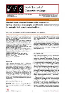
1. Introduction OCT is based on interferometry principle. OCT imaging technique has resolution in the μm range and depth of imaging in the mm range as shown in fig.1. Unlike other techniques that use X-rays, OCT is comparatively safer as it uses light source where no radiations are involved. OCT can be used to image various aspects of biological tissues. [1] Some of these include structural information, blood flow, polarization sensitivity, elastography, spectroscopy etc. Any combination of above imaging modes can be used to bring out specific features of biological tissues as desired. [1]

1877-0509 © 2015 The Authors. Published by Elsevier B.V. This is an open access article under the CC BY-NC-ND license (http://creativecommons.org/licenses/by-nc-nd/4.0/). Peer-review under responsibility of scientific committee of International Conference on Advanced Computing Technologies and Applications (ICACTA-2015). doi:10.1016/j.procs.2015.03.121

Yogesh Rao et al. / Procedia Computer Science 45 (2015) 644 – 650

645

Fig.1. Comparison of various techniques with respect to resolution and penetration depth

The Michelson interferometer setup consists of consists of a broadband source, which is split by the beam splitter along the reference arm and the sample arm. The reference arm consists of mirror and the sample arm consists of sample used for imaging. The backscattered light from the sample and reference arm are collected and allowed to interfere. This interference pattern is detected by photo detector. The source, sample, reference arm and the detector are connected to the beam splitter via optical fibers, allowing light to pass through it. Fig. 2 shows the Michelson interferometer setup.

Fig.2. Optical Coherence Tomography using Michelson Interferometer

OCT systems can be classified briefly into TD-OCT (Time domain) and FD-OCT (Frequency domain). 1) TD-OCT: It is also called first generation OCT. In TD-OCT the interference pattern is obtained by moving the reference mirror linearly, to change the reference path length and match multiple optical paths due to reflections within the sample. [1-3] 2) SD-OCT: In spectral domain OCT the reference arm is not movable. The main advantage of this method is faster acquisition rates as compared to time domain method and there are no moving parts thereby minimizing distortions. Fig. 3 shows the block diagram of SD-OCT setup.

Fig.3. OCT Setup

646

Yogesh Rao et al. / Procedia Computer Science 45 (2015) 644 – 650

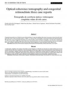
The source used is broadband source e.g. SLD (Super Luminescent diode). The beam of light coming from SLD is splitted and given to reference and sample using 50:50 beam splitter. The interference pattern is detected by spectrometer which internally has diffraction grating and CCD. Finally, the data is been sent to PC for image reconstruction. To get a 2 D image, a galvano scanner can be used which scans the sample in x-y direction. By taking the axial scans in x and y directions, one can get 2D or 3D images. Fig.4 shows the implemented hardware setup.

Fig.4. (a) OCT Setup (b) Galvano scanner

2.

Modeling of OCT

To simulate the behavior of OCT we need to know various parameters that influence the interference pattern. These parameters include coherence length, center wavelength of source(nm), half bandwidth of source(nm), power of source(nw), responsivity of detector, number of reflectors in the sample, number of samples for constructing the signals. 1) Coherence length: It is the distance travelled by wave in Tc amount of time, where Tc is coherence time. The coherence time is the time over which a propagating wave may be considered coherent. In other words, it is the time interval within which its phase is, on average, predictable. In long-distance transmission systems, the coherence time may be reduced by propagation factors such as dispersion, scattering, and diffraction. (1)

‫ ܿܮ‬ൌ ሼܿ ‫ܿܶ כ‬ሽ Where c = speed of light. Lc can also be expressed as in equation ఒమ

‫ ܿܮ‬ൌ ቄ ቅ ଶగοఒ Where οߣ =ሼ݉ܽ‫ ݔ‬െ ߣ݉݅݊ሽ ; οߣrepresents the bandwidth of the SLED source.

(2)

2) Light source spectrum : It is denoted by S(k). It denotes the spectrum of source used for OCT. [3] ܵሺ݇ሻ ൌ ݁ ିቄ ଶగ

Where k0 =

ఒ଴

ೖషೖబ మ ቅ  οೖ

*ቄ

ଵ

ο௞‫כ‬ξగ

ቅ

also called as wave number, λ0 is central wavelength of source selected.

(3)

647

Yogesh Rao et al. / Procedia Computer Science 45 (2015) 644 – 650

3) Interference Pattern: The interference pattern form by the back reflections from the reference and sample is given as [3]:

ߩ ‫ܫ‬ሺ݇ሻ ൌ  ሾܵሺ݇ሻሺܴோ ൅  ܴௌଵ ൅  ܴ௦ଶ ൅ ‫ ڮ‬ሻሿ Ͷ ୒ ߩ ൅ ሾሺሻ ෍ξ ୖ  ୗ౤ ሺ‡୧ଶ୩൫୸౎ ି୸ୗ౤ሻ൯ ൅  ‡ି୧ଶ୩ሺ୸౎ ି୸ୗ౤ሻ ሻሿ Ͷ ୬ୀଵ ே

ߩ ൅ ൥ܵሺ݇ሻ ෍ ξ ୱ୬  ୗౣ ሺ‡୧ଶ୩൫୸౏౤ ି୸ୗౣሻ൯ ൅  ‡ି୧ଶ୩ሺ୸౏౤ ି୸ୗౣሻሻ ൩ Ͷ ௡ஷ௠ୀଵ

(4) As shown in fig.5 [3], RR is reflectivity of reference arm and Rsn is reflectivity of nth reflector in sample,ߩ is responsivity of detector ,ϒ is inverse fourier transform of S(k), zR is the distance of reference arm from beam splitter and zsn is distance of nth reflector from beam splitter. ID(Z) has three terms, D.C term, autocorrelation and cross correlation terms. The D.C and autocorrelation terms are undesired terms. The autocorrelation term has least magnitude of all terms so it can be neglected. However, D.C has highest magnitude and so it needs to be filtered out.

Fig.5. OCT Schematic of Michelson interferometer used in OCT

4) Domain Transform: The interference produced, are detected by spectrometer which is function of wavelength. Dispersion results from the non-linear function of the phase dependency of wavelength λ. Therefore, the spectrometer output must be transformed from the wavelength to the other space. The factor Si nonlinearity constant is first calculated. [1]

(5) Where N is number of samples generates by ADC convertor of spectrometer. If t= (ߣ ƒš െߣ݉݅݊ሻ, Si= (N-1) – i*t+ i2*(t2-t) / (N-1) +i3 *(t3-4t2+5t-(4/ߣ݉݅݊))/ (N-1)2

(6)

It is of the form: (7)

648

Yogesh Rao et al. / Procedia Computer Science 45 (2015) 644 – 650

For the corresponding Si, ߣ݅can be found out as shown in equation (8)

(8) 5) Virtual OCT (VOCT) : As shown in fig.6, a GUI was designed using Lab VIEW and Math scripts [4], to accept the control parameters from user for simulation. These parameters include center wavelength of source(nm), half bandwidth of source(nm), power of source(nW), responsivity of detector, number of reflectors in the sample, knob for controlling number of samples for constructing the signals(range :0 to 1000). The various indicators displayed are SLD (source) spectrum, Si non linearity constant graph versus the number of samples, λ to k- domain transform, interference pattern and imaging of ‘A’ scan. Several A scans can be combined together to form a 3 D image called ‘B’ scan. The block diagram for the simulation in Lab VIEW is as shown in fig.7. Here, the sub VI calculates all the values of Si, Interference pattern, SLD spectrum, IFFT, Ki versus wavelength and displays it on waveform graph.

Fig.6. GUI of VOCT

Fig.7. Block diagram of VOCT

Yogesh Rao et al. / Procedia Computer Science 45 (2015) 644 – 650

6) Results: For center wavelength=1310nm, half bandwidth=50nm, power of source=10 mW, responsivity=0.001, number of reflectors=4, number of samples=600, the SLD spectrum is as shown in fig.8. Here the spectrum is spread across kmax and kmin corresponding to max and min. These values are been provided as inputs by user during simulation. Fig.9 shows the graph for Si versus number of samples. As Si is been calculated to compensate for nonlinearity, from the graph it can be seen that the response is linear. Fig.10 shows the graph for Ki versus wavelength. It corresponds to to k transform for every value of . Fig.11 shows the interference pattern plotted. Fig.12 shows the IFFT of the interference pattern. It can be seen that the D.C component has the largest amplitude which is centered at zero frequency. The four impulses correspond to the four reflector layers. The lowest amplitude terms corresponds to autocorrelation terms. Fig.13 shows the simulated image without filtering out the undesired D.C and autocorrelation terms for four layers. Fig.14 shows the simulated image with filtering out the undesired terms.

Fig.8.SLD Spectrum

Fig.9. Si versus number of samples

Fig.10. Ki versus wavelength

Fig.11. Interference pattern

Fig.12. IFFT of interference pattern

649

650

Yogesh Rao et al. / Procedia Computer Science 45 (2015) 644 – 650

Simulated image after removing D.C terms & Auto correlation

Simulated image with D.C Terms & Auto correlation Terms 0.5

0.5

0.6

0.6

0.7

0.7

0.8

0.8

0.9

0.9

1

1

1.1

1.1

1.2

1.2

1.3

1.3

1.4

1.4

1.5

50

100

150 samples----->

200

Fig.13. Simulated image without filtering

250

1.5

50

100

150 samples----->

200

250

Fig.14. Simulated image with filtering

7) Conclusion To carry out real time OCT for human samples, VOCT software was designed. VOCT carries out simulation to plot the interference pattern of ‘A’ scan and its simulated images. The software can be further modified to import real time ‘A’ scan data of any sample from spectrometer and form a simulated depth resolved image. Scanning in z direction would result in 3D image reconstruction. The main objective is to have a miniaturized setup comprising of interferometer, source, reference and sample arm, and detector. The data of spectrometer will be exported to VOCT where signal processing of data like noise removal, k transform calculation of Si will be carried out. Finally a 2D image will be formed so as to get depth resolved information of sample.

8) References 1. Murtaza Ali and Renuka Parlapalli, “Signal Processing Overview of Optical Coherence Tomography Systems for Medical Imaging,” TEXAS INSTRUMENTS, SPRABB9–June 2010. 2. Peng Li, Yonghong He, Hui Ma, “Spectral-Domain Optical Coherence Tomography and Applications for Biological Imaging,” IEEE(2006). 3. J.A. Izatt and M.A. Choma, “Theory of Optical Coherence Tomography,” Optical Coherence Tomography Technology and Applications, Springer,pp.47-72. 4. Image processing toolbox help, MATLAB® [Online]. Available: http://www.mathworks.com/