The SAWs are excited by interdigital transducers and are diffracted into the device where they propagate through the base and enter the fluid filled microchannel ...
Modeling and Simulation of Piezoelectrically Agitated Acoustic Streaming on Microfluidic Biochips Harbir Antil1 , Andreas Gantner2 , Ronald H.W. Hoppe1,2 , Daniel K¨ oster2 , 2 3 Kunibert Siebert , and Achim Wixforth 1
2
3
University of Houston, Department of Mathematics (http://www.math.uh.edu/~rohop/) University of Augsburg, Institute for Mathematics (http://scicomp.math.uni-augsburg.de) University of Augsburg, Institute of Physics (http://www.physik.uni-augsburg.de/exp1)
Summary. Biochips, of the microarray type, are fast becoming the default tool for combinatorial chemical and biological analysis in environmental and medical studies. Programmable biochips are miniaturized biochemical labs that are physically and/or electronically controllable. The technology combines digital photolithography, microfluidics and chemistry. The precise positioning of the samples (e.g., DNA solutes or proteins) on the surface of the chip in pico liter to nano liter volumes can be done either by means of external forces (active devices) or by specific geometric patterns (passive devices). The active devices which will be considered here are nano liter fluidic biochips where the core of the technology are nano pumps featuring surface acoustic waves generated by electric pulses of high frequency. These waves propagate like a miniaturized earthquake, enter the fluid filled channels on top of the chip and cause an acoustic streaming in the fluid which provides the transport of the samples. The mathematical model represents a multiphysics problem consisting of the piezoelectric equations coupled with multiscale compressible Navier-Stokes equations that have to be treated by an appropriate homogenization approach. We discuss the modeling approach and present algorithmic tools for numerical simulations as well as visualizations of simulation results.
1 Introduction Microfluidic biochips and microarrays are used in pharmaceutical, medical and forensic applications as well as in academic research and development for high throughput screening, genotyping and sequencing by hybridization in genomics, protein profiling in proteomics, and cytometry in cell analysis (see [7]). Traditional technologies such as fluorescent dyes, radioactive markers, or nanoscale gold-beads only allow a relatively small number of DNA probes per assay, and they do not provide information
306
H. Antil et al.
about the kinetics of the processes. With the need for better sensitivity, flexibility, cost-effectiveness and a significant speed-up of the hybridization, the current technological trend is to integrate the microfluidics on the chips itself. A new type of nanotechnological devices are Surface Acoustic Wave (SAW) driven microfluidic biochips (cf. [4, 9]).
Fig. 1. Microfluidic biochip with network of microchannels (left), and sharp jet created by surface acoustic waves (right) The experimental technique is based on piezoelectrically actuated Surface Acoustic Waves (SAW) on the surface of a chip which transport the droplet containing probe along a lithographically produced network of microchannels to marker molecules placed at prespecified surface locations (cf. Fig. 1 (left)). These microfluidic biochips allow the in-situ investigation of the dynamics of hybridization processes with extremely high time resolution. The SAWs are excited by interdigital transducers and are diffracted into the device where they propagate through the base and enter the fluid filled microchannel creating a sharp jet on a time-scale of nanoseconds (cf. Fig. 1 (right)). The acoustic waves undergo a significant damping along the microchannel resulting in an acoustic streaming on a time-scale of milliseconds. The induced fluid flow transports the probes to reservoirs within the network where a chemical analysis is performed.
2 Modeling of SAW Driven Microfluidic Biochips Mathematical models for SAW biochips are based on the linearized equations of piezoelectricity in Q1 := (0, T1 ) × Ω1 ρ1
∂ 2 ui ∂ ∂uk ∂ − cijkl ekij − ∂t2 ∂xj ∂xl ∂xj ∂uk ∂ ∂ ejkl ǫjk − ∂xj ∂xl ∂xj
∂Φ =0, ∂xk ∂Φ =0 ∂xk
(1a) (1b)
with appropriate initial conditions at t = 0 and boundary conditions on Γ1 := ∂Ω1 . Here, ρ1 and u = (u1 , u2 , u3 )T denote the density of the piezoelectric material and the mechanical displacement vector. Moreover, ǫ = (ǫij ) stands for the permittivity
Acoustic Streaming on Microfluidic Biochips
307
tensor and Φ for the electric potential. The tensors c = (cijkl ) and e = (eikl ) refer to the forth order elasticity tensor and third-order piezoelectric tensor, respectively. The modeling of the micro-fluidic flow is based on the compressible Navier-Stokes equations in Q2 := (0, T2 ) × Ω2 ρ2
� η� ∂v + (v · ∇)v = − ∇p + η ∆v + ζ + ∇(∇ · v) , ∂t 3 ∂ρ2 + ∇ · (ρ2 v) = 0 , ∂t ∂u v(x + u(x, t), t) = (x, t) on (0, T2 ) × Γ2 ∂t
(2a) (2b) (2c)
with suitable initial conditions at t = 0 (see, e.g., [1, 2]). In the model, compressible and non-linear effects are the driving force of the resulting flow. Here, ρ2 , v = (v1 , v2 , v3 )T and p are the density of the fluid, the velocity, and the pressure. η and ζ refer to the shear and the bulk viscosity. The boundary conditions include the time derivative ∂u/∂t of the displacement of the walls Γ2 = ∂Ω2 of the microchannels caused by the surface acoustic waves. Therefore, the coupling of the piezoelectric and the Navier-Stokes equations is only in one direction. No back-coupling of the fluid onto the SAWs is considered. It has to be emphasized that the induced fluid flow involves extremely different time scales. The damping of the sharp jets created by the SAWs represents a process with a time scale of nanoseconds, whereas the resulting acoustic streaming reaches an equilibrium on a time scale of milliseconds. SAWs are usually excited by interdigital transducers located at Γ1,D ⊂ Γ1 operating at a frequency f ≈ 100 MHz with wavelength λ ≈ 40 µm. The time-harmonic ansatz leads to the saddle point problem: Find (u, Φ) ∈ V × W , where V ⊂ H 1 (Ω1 )3 , W ⊂ H 1 (Ω1 ), such that for all (w, Ψ ) ∈ V × W Z Z Z ∂Φ ¯ ¯ cijkl εkl (u)εij (w)dx − ω 2 ρ1 ui w ¯i dx + ekij εij (w)dx = < σ n , w >, ∂xk Z
Ω1
Ω1
eijk
Ω1
∂ Ψ¯ dx εij (u) ∂xk
−
Ω1
Z
ǫij
∂Φ ∂ Ψ¯ dx ∂xi ∂xj
= < Dn , Ψ > .
Ω1
Here, (εij (u)) stands for the linearized strain tensor and ω = 2πf . The elastic 1 and electric Neumann boundary data are supposed to satisfy σ n ∈ H − 2 (Γσ )2 and 1 −2 Dn ∈ H (ΓD ) with < ·, · > in the above system denoting the respective dual products. Then, the following results holds true (cf. [3]): Theorem 1. For the above saddle point problem, the Fredholm alternative holds true. In particular, if ω 2 is not an eigenvalue of the associated eigenvalue problem, there exists a unique solution (u, Φ) ∈ V × W . In order to cope with the two time-scales character of the fluid flow in the microchannels (penetration of the SAWs within nanoseconds and induced acoustic streaming within milliseconds), we perform a separation of the time-scales by homogenization. In particular, we consider an expansion of the velocity v in a scale parameter ε > 0 representing the max´ımal displacement of the walls
308
H. Antil et al. v = v0 + ε v′ + ε2 v′′ + O(ε3 )
and analogous expansions of the pressure p and the density ρ2 . We set v1 := εv′ , v2 := ε2 v′′ and define pi , ρ2,i , 1 ≤ i ≤ 2, analogously. Collecting all terms of order O(ε) results in the linear system ρ2,0
� ∂v1 η� − η ∆v1 − ζ + ∇(∇ · v1 ) + ∇p1 = 0 ∂t 3 ∂ρ2,1 + ρ2,0 ∇ · v1 = 0 ∂t ∂u p1 = c20 ρ2,1 in Q2 , v1 = ∂t
in Q2 ,
(3a)
in Q2 ,
(3b)
on Γ2 ,
(3c)
where c0 represents the small signal sound speed in the fluid. The system describes the propagation of damped acoustic waves. Collecting all terms of order O(ε2 ) and performing the time-averaging hwi := R t +T T −1 t00 w dt, where T := 2π/ω, we arrive at the Stokes system in Ω2 � η� ∂v1 −η ∆v2 − ζ + − ρ2,0 [∇v1 ]v1 i , ∇(∇ · v2 ) + ∇p2 = h−ρ2,1 3 ∂t ρ2,0 ∇ · v2 = h−∇ · (ρ2,1 v1 )i , v2 = − h[∇v1 ]ui
on Γ2 .
(4a)
(4b) (4c)
The Stokes system describes the stationary flow pattern, called acoustic streaming, resulting after the relaxation of the high frequency surface acoustic waves. As far as analytical results for the Navier-Stokes equations (3a)-(3c) are concerned, one can show existence and uniqueness of a weak periodic solution assuming the forcing term to be a periodic function. Moreover, under some extra regularity assumption it can be shown that the periodically extended solution converges to an oscillating equilibrium state (see [5]). Theorem 2. Assume that the forcing term is a periodic function of period T . Then, the linear Navier-Stokes equations (3a)-(3c) have a unique weak periodic solution (vper , pper ) ∈ H 1 ((0, T ); H −1 (Ω)3 × L20 (Ω)). Moreover, if (˜ v, p˜) resp. (˜ vper , p˜per ) are extensions of the solution resp. the periodic solution of the Navier-Stokes equation with periodic forcing term to arbitrary large 2 2 2 2 ˜ , ∂tt ˜ per , ∂tt τ > 0 and if (∂tt v p˜), (∂tt v p˜per ) ∈ L2 ((0, τ ); H), where H := L2 (Ω)3 × L20 (Ω), then there holds k(˜ v(t), p˜(t)) − (˜ vper (t), p˜per (t))kH = O(t−1/2 ) .
3 Simulation of the SAWs and the Microfluidic Flows The time-harmonic acoustic problem is solved in the frequency domain by using P1 conforming finite elements with respect to a hierarchy of simplicial triangulations. This leads to an algebraic saddle point problem � � � �� � Aω B f U . (5) = T g Φ B −C
Acoustic Streaming on Microfluidic Biochips
309
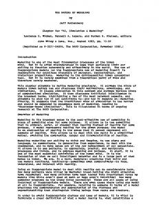
For the numerical solution of (5) we use multilevel preconditioned CG for the associated Schur complementbased on a block-diagonal preconditioner � −1 � A˜ω 0 P −1 = (6) −1 ˜ 0 C with BPX- or hierarchical-type preconditioners for the stiffness matrices associated with the mechanical displacement and electric potential, respectively (see [3] for details). 3000
2500
400
Standard FEM Hierarchical Basis BPX
Standard FEM Hierarchical Basis BPX
# Iterations
# Iterations
300 2000
1500
1000
200
100 500
0 1
2
3
4
5
6
Refinement Level
7
8
9
0 1
2
3
Refinement Level
4
5
Fig. 2. Performance of the multilevel preconditioned CG compared with standard CG in 2D (left) and 3D (right) Fig. 2 displays the performance of the multilevel preconditioners compared to the standard single-grid iterative solver both in 2D (on the left) and in 3D (on the right). For the BPX-preconditioner we observe the expected asymptotic independence on the refinement level (cf., e.g., [6]). The Navier Stokes equations (3a)-(3c) with a periodic excitation on the boundary Γ2 are discretized in time by the Θ-scheme (cf., e.g., [8]), until a specific condition for periodicity of the pressure is met. The discretization in space is taken care of by Taylor-Hood elements with respect to a hierarchy of simplicial triangulations. On the other hand, for the discretization of the time-averaged Stokes system we use the same techniques as for the time-harmonic acoustic problem (see [5] for details).
4 Numerical Simulation Results The following simulation results are based on 2D computations that have been carried out for LiNbO3 as the piezoelectric material and assuming the fluid in the microchannels to be water at 20◦ C. For a precise specification of the geometrical and material data we refer to [3] and [5]. Fig. 3 shows the amplitudes of the electric potential at an operating frequency of 100 MHz (left) and the polarized Rayleigh waves by means of the displacement vectors (right). The amplitudes of the displacement waves are in the region of nanometers. The SAWs are strictly confined to the surface of the substrate. Their penetration depth into the piezoelectric material is in the range of one wavelength. Rayleigh surface waves characteristically show an
310
H. Antil et al.
elliptical displacement, i.e., the displacements in the x1 - and x2 -direction are 90o out of phase with one another. Additionally, the amplitude of the surface displacement in the x2 -direction is larger than that along the SAW propagation axis x1 .
Fig. 3. Electric potential wave (100 MHz) (left) and mechanical displacement vectors (right) Fig. 4 (left) displays the effective force creating the sharp jet in the fluid (cf. Fig. 1 (right)) which can be easily computed by means of F := ρ2,0 h(v1 ·∇)v1 +v1 (∇·v1 )i, where the brackets stand for the time average removing the fast oscillations of the sound wave. Fig. 4 (right) contains a visualization of the associated velocity field.
Fig. 4. Effective force and associated velocity field Fig. 5 shows the strong damping of the acoustic waves in the fluid where excitation occurs through an SAW running from left to right along the lower edge at a frequency of 100 MHz. We have performed a model validation by a comparison of experimental data with numerical simulation results. Fig. 6 (left) displays the measured streaming pattern visualized by a fluorescence video microscope for an experimental layout consisting of a typical biochip with an IDT placed on top of a standard YXl 128ˆ o substrate (the IDT is visible at the bottom right of Fig. 6 (left)). Fig. 6 (right) shows the result of a
Acoustic Streaming on Microfluidic Biochips
311
Fig. 5. Strong damping of the SAWs after penetration into the fluid
Fig. 6. Model validation: experimental measurements (left) and numerical simulation results (right)
simulation run based on the data of the experimental setting. A similar qualitative behavior can be observed. More importantly, for the resulting acoustic streaming the simulation results are quantitatively in good agreement with the experimental data. Acknowledgement. The authors acknowledge support by the German National Science Foundation within the Priority program ‘Optimization with Partial Differential Equations’. The work of the first author is further partially supported by the NSF under Grant-No. DMS-0511611.
References [1] C.E. Bradley. Acoustic streaming field structure: The influence of the radiator. J. Acoust. Soc. Am., 100:1399–1408, 1996.
312
H. Antil et al.
[2] B. Desjardins and C.-K. Lin. A survey of the compressible Navier-Stokes equations. Taiwanese Journal of Mathematics, 3:123–137, 1999. [3] A. Gantner, R.H.W. Hoppe, D. K¨ oster, K. Siebert, and A. Wixforth. Numerical simulation of piezoelectrically agitated surface acoustic waves on microfluidic biochips. Comput. Vis. Sci., 10(3):145–161, 2007. [4] Z. Guttenberg, H. M¨ uller, H. Haberm¨ uller, A. Geisbauer, J. Pipper, J. Felbel, M. Kilepinski, J. Scriba, and A. Wixforth. Planar chip device for pcr and hybridization with surface acoustic wave pump. Lab Chip, 5:308–317, 2005. [5] D. K¨ oster. Numerical simulation of acoustic streaming on saw-driven biochips. Dissertation, Inst. of Math., Univ. Augsburg, 2006. [6] P. Oswald. Multilevel Finite Element Approximations: Theory and Applications. Teubner, Stuttgart, 1994. [7] J. Pollard and B. Castrodale. Outlook for dna microarrays: emerging applications and insights on optimizing microarray studies. Report. Cambridge Health Institute, Cambridge, 2003. [8] J.W. Thomas. Numerical Partial Differential Equations: Finite Difference Methods. Springer, Berlin-Heidelberg-New York, 1995. [9] A. Wixforth, C. Strobl, C. Gauer, A. Toegl, J. Scriba, and Z. Guttenberg. Acoustic manipulation of small droplets. Anal. Bioanal. Chem., 379:982–991, 2004.