Modeling and Simulation of Time Domain Faults in Digital Systems D. Barros Júnior1, F. Vargas1, M. B. Santos2, I. C. Teixeira2 and J. P. Teixeira2 1 PUCRS, Porto Alegre, Brazil; 2 IST / INESC-ID Lisboa, Portugal
[email protected],
[email protected]
Abstract The purpose of this paper is to present and discuss a novel modeling and fault simulation technique for two types of dynamic faults in digital systems: transient power supply voltage drops and transient delays in logic elements or signals paths. Techniques and tools currently used for permanent faults are reused for dynamic (permanent) and intermittent faults. For transient power supply voltage drops (∆VDD), two approaches are proposed: delay fault injection in all logic elements of the CUT (Circuit Under Test), or modulation of the clock and observation rate. For transient delays (e.g., SEU), single delay injection is performed at logic element level. Delay modulation is carried out by fault injection using the PLI interface of the commercial Verilog simulation tool. Preliminary results, demonstrated by the c7552 ISCAS’85 benchmark circuit, show that CUTs with long critical paths are very sensitive to power supply transients. Moreover, a pseudo-random test pattern can be used to identify the dependence of the CUT sensitivity to delay faults on defect size, for a given clock period, τo.
1. Introduction High quality products require high-quality production test. Highly dependable products (for safety-critical or economically-critical applications) require tolerance to defects and environmental disturbances. Defects and disturbances are modeled as faults. Fault injection campaigns are required, during new product development, to evaluate and improve design and test quality. Defects, induced during manufacturing or product lifetime, or environmental disturbances (e.g., power supply voltage transients [1], or Single Event Upset (SEU) and Transients (SET)) may cause permanent faults and/or intermittent faults. Permanent faults can further be categorized into static (e.g., single Line StuckAt (LSA) faults) or dynamic, such as delay faults. The detection of static faults has been extensively investigated, and mature methodologies and tools are available for digital systems. Dynamic faults and intermittent faults are the focus of this work, as well as high-speed products, for which the clock rate is pushed to the limit allowed by the manufacturing technology and process variations. Fault modeling and simulation, performed in a cost effective way, can be useful for two, complementary objectives: either to develop fault-
tolerant products, or to develop high-quality tests to uncover the target faults. Delay testing for digital systems has been a topic of intensive research [1-13], with emphasis on permanent delay faults. As new, emerging nanometer technologies become mainstream technologies, testing to uncover dynamic faults is becoming even more relevant, especially when high-quality, low DPM (Defects Per Million) products are considered [3]. Moreover, the sensitivity of semiconductor devices to environmental disturbances increases with device scaling down. Consider a permanent or intermittent delay fault, either local or global, characterized by a defect size – the delay deviation, ∆τ. Here, we refer as local delay faults those affecting a single Logic Element (LE) or interconnection in the circuit, while global delay faults are the ones affecting all LEs. ∆VDD (SEU/SET) faults are expected to induce global (local) delay faults. In order to cause a system timing failure, the defect size of the delay fault(s) must exceed the signal path slack. The path slack is defined as the difference between the time allowed for signal propagation (the clock period, τo) and the path length. The signal path delay considers the delays of all the logic elements and all the interconnection delays in the path [14]. In this work, delay faults on combinational circuits are under investigation. Two types of relevant dynamic faults in digital systems are considered: transient power supply voltage drops (∆VDD) (important for EMI/EMC standard compliance [15], and for power supply noise monitoring [1]) and transient delays in logic elements or signals paths. Here, we assume that their impact does not cause a functional error (incorrect logic values at the system primary outputs), but it may cause a performance error (incorrect time response, leading to a timing failure). Hence, we assume that such dynamic faults manifest themselves as delay faults (permanent, or intermittent). One may argue that we approach a complex, challenging problem with a too simplistic model. However, the objective is, by addressing only this valued characteristic of the abnormal behavior, we may draw conclusions on its impact, both for fault tolerance and for fault detection. Fault injection of such faults is not a trivial task. The purpose of this work is to propose a cost-effective modeling and fault simulation scheme for such dynamic faults, using a commercial simulation platform. Sections 2 and 3 describe the modeling and simulation techniques, section 4 presents typical results and section 5 summarizes the main conclusions of the work.
2. Fault Modeling Approach Consider a Circuit Under Test (CUT) to which a pseudo-random (PR) test pattern is applied. PR test vectors are applied using a clock rate τo, and responses are observed at the same rate. A defect or disturbance is assumed to modify the typical delay, globally or locally, inducing (or not) a timing failure at its PO (Primary Outputs). The proposed modeling approach does not depend on actual test stimuli. However, experiments have been carried out with PR test for good reasons. In fact, a PR test sequence, being pseudo-random, is not biased to detect difficult transient faults, as this is not the objective of the work. Unbiased PR sequences (generated, e.g., by a LFSR (Linear Feedback Shift Register)) are used in this work (1) to find out if such a unbiased test can nevertheless provide a low-cost snapshot of the circuit timing behavior, namely the identification of the most relevant CUT logic elements likely to induce timing failures, and of a first set of input transitions (test vector pairs) which are useful to detect the timing failures under consideration; (2) such PR test is well suited for BIST (Built-In Self Test) implementation, which could prove to be rewardingly used for testing such defects or disturbances. Assume first that the CUT experiences a transient VDD voltage drop. At logic level, the VDD variable is absent. Hence, we need to model the impact of such transient on CUT behavior. Under this disturbance, signals temporarily undergo lower voltage swings and the driving strength of pull-up / pull-down paths (network of NMOS/PMOS field-effect transistors) is reduced, while the parasitic capacitances remain unchanged. Consequently, each logic element will exhibit an increased time response, and the CUT’s response exhibits an abnormal delay (see Figure 1 for a typical example). The characteristics of the VDD transient (pulse width, ∆τ, and magnitude, ∆VDDmax) will determine the quantitative modification on the timing response. Here, we distinguish between two situations, both from a timing and voltage level points of view: slow and fast transient (as compared to the clock period, τo); moderate and sharp transitions (as compared to nominal VDD values). Accurate quantification of these domains is considered out of the scope of this paper. However, a moderate transition requires that the VDD voltage drop is not too severe, allowing correct gate Boolean behavior. Therefore, we assume that low VDD(t) values are always greater than a given threshold value. For the sake of comprehensiveness, we assume that VDD (t)min > 2.5 Vth, where Vth is the average threshold voltage of NMOS/PMOS transistors in the target IC technology. In order to have an idea of the dependence of logic elements delays (defect size) on the VDD value, we can
use the approximate equation for the propagation delay of a CMOS inverter, Td, as used in [8], Td = K. VDD / (VDD – Vth)2, where K = CL / (µ Cox (W/L)) and the symbols retain the usual meaning. Assume that, for the target technology, Vth = 0.2 VDDnom. Hence, restricting VDD voltage drop to 2.5.Vt corresponds to restrict the power supply voltage transient to values as low as half of the nominal VDD value. For VDDmin = VDDnom /2, an increase of the inverter propagation delay of Td (VDD=2.5.Vt) = 3.55 Td (VDDnom) is obtained. This is a significant delay increase, although pessimistic due to the quadratic power law assumed for the MOS transistor’s ID(VGS) in saturation. Accurate modeling of the dependence of the defect size on VDD(t) is under evaluation, and will be reported in the future.
Figure 1 – 77 inverters ring oscillator (AMS 0.35 µm CMOS technology) under a slow transient ∆VDD . The impact of transient power supply voltage drops on circuit performance can thus be modeled, at logic level, as an enhanced propagation delay of all library logic elements and/or signal paths. The proposed modeling approach of such dynamic faults takes into account the rationale used on the detection of design flaws using VLV (Very Low Voltage) testing [8] and on resistive bridging fault coverage enhancement techniques using VLV testing [9]. Consider now that an intermittent delay fault occurs, e.g., due to the impact of an alpha particle, causing a Single Event Transient (SET). We assume that the signal glitch is not captured by a memory element, thus not causing a permanent bit flip. Instead, we assume that the glitch delays the correct Boolean operation performed by the signal path in which the affected logic element lies. In this situation, fault modeling requires a modification of the library-stored delay values of the single logic element affected by the disturbance.
3. Fault Simulation Approach As referred, fault simulation of the two considered types of faults is not a trivial task. First, no VDD “exists”
as variable, at logic level. Second, continuous time variations are absent of the digital simulation. Third, transient CUT modifications during simulation (to inject a temporary fault) also require tricky simulation techniques. Therefore, using commercial tools, how can we evaluate the impact of these faults on circuit performance? Prior to analyzing the fault injection process, let us look into the issue of intermittent versus permanent faults simulation. Our claim is that modeling and simulation of intermittent faults can take advantage of reusing the techniques and tools currently used for permanent faults. The simulation process is first established assuming that the abnormal delay(s) is(are) permanent. This allows us to reuse mature tools, commercially available. For a given PR test pattern, it is thus possible to estimate, through fault simulation, the detection probability of all or single path delay faults, as a function of the defect size. Each simulation experiment provides us, for each defect size and assumed clock period, τo, the failing vectors (if any) and their faulty signatures. For single delay fault injection, it can also identify the logic elements which are failing first, as the defect size increases. Such logic elements are expected to be part of the critical paths. Fault detection is, in reality, guaranteed by the input transition between two vectors: the test vector precedent to the failing vector, and the failing vector itself. Consequently, it is possible to estimate the ability of the PR test pattern to detect or tolerate the defect or disturbance under consideration. Note that estimating the detection probability through a given PR test pattern experiment has its limitations. In fact, as it can be said regarding permanent (stuck-at) faults, random pattern resistant delay faults are to be expected. In reality, such faults are resistant to the consecutive vector pairs generated in the PR test sequence. Research is under way to evaluate how reliable is the estimation of the detection probabilities based on a PR test experiment. Preliminary results suggest that, if a large test length is considered, results seem promising. Now, let us address the fault injection issue, for both types of dynamic faults under consideration. Consider first the transient VDD voltage drop. At logic level, fault injection of such delay faults would require that the timing parameters of the library logic primitives of the digital circuit are modified during simulation, either permanently, or temporarily. This is a computationally costly process, even for permanent faults. At logic level, and for combinational circuits, we propose to exploit the time excitation - delay response duality. Fault injection may be performed either by CUT faulty delay injection, or by faulty time excitation pace (clock period τ < τo ) modulation. This duality corresponds to what we call the “accordion” effect. Under the VDD transient, either the CUT performance
slows down, or the stimuli race increases. Performing the fault injection by modifying the clock period has the significant advantage of using the fault-free CUT description; hence a low-cost simulation can be carried out. Moreover, when fault injection is performed at library cells delay level, only a discrete set of defect sizes (corresponding to a discrete set of VDD values) can be sequentially be carried out. However, when fault injection is performed by clock period modulation, even a continuous variation of τo can be envisaged. Regarding the simulation process, the proposed technique uses, as kernel simulator, a commercial simulator (Verilog, from Cadence). Delay fault injection is performed through the available PLI interface, which allows to modulate library cell attributes. As, in the presence of VDD voltage drops, pullup/pull-down currents increase and capacitance values remain unchanged, fault injection is carried out modifying the rise and fall delays, the parameters used in our experiments. Therefore, for power supply voltage drops, two strategies are proposed: (1) nominal clock frequency (unchanged stimuli pace application) and faulty delay injection in all logic elements in the circuit netlist, or (2) clock frequency modulation (to simulate abnormal circuit delays) and unchanged (fault-free) circuit description. Consider now that an intermittent delay fault occurs, e.g., due to a SET. Assuming that the signal glitch delays the Boolean operation performed by the signal path in which the affected logic element lies, fault injection needs to be performed by modifying locally the librarystored delay values of the single logic element affected by the disturbance.
3. Results The proposed modeling and simulation approach for these transient timing failures is validated (in its preliminary results) using as test vehicle an ISCAS’85 benchmark circuit, the c7552, and a PR test sequence. The c7552 benchmark circuit [17] has 207 primary inputs, 108 primary outputs, 876 inverters, 2636 gates (1310 ANDs + 1904 NANDs + 244 ORs + 54 NORs) and 534 buffers. A PR test pattern of test length up to 65,000 test vectors has been used. The structural Verilog description used has 2051 logic elements in which delay faults can be injected. For the experiments, simultaneous percentage increase in rise and fall time (∆τr ,∆τf) have been injected. Defect sizes range from 0.9% up to 60%. Library cells are from an AMS 0.35 µm CMOS technology with nominal VDD = 3.3 V. Circuit level fault simulation results are not included, due to space limitations. 3.1 Fault-free Simulations
First, the fault-free logic simulation has been performed and the clock frequency increased until a timing failure (for the PR test pattern) occurs. This allowed us to identify 7.48 ns as the nominal clock period for this circuit and technology In order to study the sensitivity of the CUT to delay faults, a stringent value for the clock period has been selected: τo = 7.6 ns. With this time frame, the CUT starts to exhibit timing failures when the clock period is reduced 1.6%. As shown in Figure 2, applying the first 5,000 PR test vectors a reduced set of test vectors pairs (identified by the number of the 2nd. vector) make timing failures visible at the primary outputs of the benchmark circuit. In these experiments, the clock period starts at 8 ns, and 0.5% decrease in the clock period is applied in sequence. For a better understanding of the Figure, clock values (in ns) are grouped into ranges: [7.44 – 7.40], and so on. For 7.48 ns, the output is fault free. For 7.44 ns, two vector pairs (#4363 and 4859) allow observation of a timing failure. We refer these test vector pairs as timing vectors, in the sense that these input transitions allow the identification of time-limited behavior at the CUT’s outputs. Timing vectors are associated with the activation of signal critical paths. As the clock period decreases, the number of failing vectors monotonically increase (2, 3, 10, 12, 25 and 32). For this benchmark and PR test, the two most “fruitful” timing vector are #4363 and 4859. As shown in Figure 2, an “iceberg like” behavior can be observed. As the clock period is being reduced, first two timing vectors are identified, then (in the [7.20 – 7.29] range) additional four (#4295, 4791, 4818 and 4826), then (in the [7.00 – 7.09] range) additional five (#2327, 4308, 4428, 4627, and 4832), and finally (in the [6.90 – 6.99] range) additional five (# 2207, 2267, 4039, 4762 and 4799) timing vectors are identified. When injecting the faults, the set of timing vectors should be monitored, as we expect that abnormal delays in the circuit behavior will likely produce timing failures in the same vector pairs. 3.2 Multiple Delay Fault Injection (∆ ∆VDD Faults) Fault injection for the power supply voltage drop faults has been subsequently performed, according to the two strategies described above. Delay fault injection in all library logic elements has been performed, by incrementing (∆τr ,∆τf) in steps of 0.9% (Figure 3). With just 2.7% increase, and the τo = 7.60 ns timeframe, the CUT exhibited a timing failure in 2 out of the first 5,000 vectors, again in the “fruitful” timing vectors, #4363 and 4859. The number of failing vectors again monotonically increases with the defect size. It is interesting to compare the “iceberg-like” behavior again, leading to the identification of basically the same timing vectors (and by the same order of occurrence) as in the fault-free
simulation, which ascertains the time excitation - delay response duality assumption. In fact, as the defect size is being increased, the same first two timing vectors are identified, then (in the [4.5 – 5.4] range) additional four (#4295, 4791, 4818 and 4826), then (in the [8.1 – 9.0] range) additional seven (#2207, 2267, 2327, 4308, 4428, 4627, and 4832), and finally (in the [9.9 – 10.8] range) additional seven (# 4002, 4039, 4603, 4762, 4799, 4840 and 4900) timing vectors are identified. As it can be seen, for large defect sizes, some additional timing vectors are identified, which may indicate that the model of percentage increase may finally transform some noncritical paths into critical paths, under low VDD conditions. As referred, ∆VDD faults are expected to lead to relatively large delay increase per gate, as it can also be observed in the delay versus VDD dependence on a given cell library. The cumulative delay build through a critical path justifies the fact, confirmed by simulation, that CUTs (like this one) with long critical paths are very sensitive to this intermittent disturbance. High performance VLSI circuits, such as microprocessors, typically have short critical paths between logic elements. The delay fault simulation results supports the conclusion that such high-performance devices exhibit (fortunately) a lower sensitivity to ∆VDD drops, as compared to modules such as the c7552. Data showing the dependence of the number of failing vectors, ni, on the percentage increase of (∆τr ,∆τf), can be used for the estimation of the detection probability of a given ∆VDD voltage drop fault on the defect size. In fact, the detection probability for a permanent low VDD operation can be estimated, for the specific PR test sequence, as ni / N, where N is the number of applied vectors. When an intermittent VDD voltage drop disturbance occurs, the probability of a timing failure to occur is further reduced. Note that, for the 5,000 PR test sequence, only 20 out of 5,000 vectors lead to timing failures (for 10% increase of (∆τr ,∆τf), which allow us to conclude that, for short time VDD drops, the CUT seems to be relatively tolerant to this disturbance. Of course, we must keep in mind that no test sequence, optimized for the detection of delay faults, has been applied to the CUT; hence, some hard to detect delay faults may not be uncovered by this 5,000 vectors PR test pattern. However, hard to detect permanent faults will be even harder to detect, if they occur during a very limited period of time. 3.3 Single Delay Fault Injection Another set of experiments has been performed for single (∆τr ,∆τf) fault injection in each of the 2051 library logic elements, again using the τo = 7.60 ns timeframe. Building the whole delay fault dictionary is
time consuming, even for this small benchmark circuit, especially if we want to collect all failing vectors for all 65,000 vectors. Preliminary results have been obtained with 50% increase on single (∆τr ,∆τf) fault injection on randomly chosen 500 logic elements (out of the total of 2051), using 5,000 PR vectors. Simulation stops analyzing one delay fault when the first failing vector is identified. Even with such large delay increase (50%), only 3 out of the 500 logic elements (LE # 1, 3 and 262) have produced timing failures. Additional detailed results have been obtained, and are shown in Figure 4. Now for all the 2051 logic elements in the CUT, single local delay faults have been injected, using only the first 5,000 PR vectors. Five defect sizes (25, 30, 40, 50 and 60% increase of rise and fall delays) have been injected. As shown in Figure 4, the “iceberg like” behavior is again observed, and with the same “shape” as before. The main difference is now that the single fault situation requires a much large defect size. This conclusion is reasonable, as the increase path delay needed to erode the path slack is now lumped into a single logic element, instead of being distributed as % increase in all logic elements in the path. In fact, as the single defect size is being increased, the same first two timing vectors are identified, then (for 40%) additional four (#4295, 4791, 4818 and 4826), then (for 60%) additional five (#2327, 4308, 4428, 4627 and 4832), timing vectors are identified. Now, not only the timing vectors, but also the logic elements in which abnormal delays are injected, can be identified by simulation. Additional information can be extracted from the faulty signatures, identifying the primary outputs which terminate these critical paths.
4. Conclusions In this paper, a novel modeling and fault simulation technique for two types of dynamic faults in digital systems has been proposed, for (1) transient power supply voltage drops and (2) transient delay faults in logic elements or signals paths. The innovative ideas emerge from the following concepts: reuse (for intermittent faults) of methodologies and tools for permanent faults, modeling of ∆VDD voltage drops as % increased delays in all logic elements, delay fault simulation performed by exploiting the time excitation - delay response duality, and single or multiple delay fault injection on a commercial simulator using its PLI interface. Future work encompasses defect size computation, as a function of the VDD(t) pulse characteristics, minimum allowable VDD values for only-performance impact, test of sequential CUTs and validation through extensive electric level (SPICE-like) fault simulation.
References [1] A. Krstic, Y-M. Jiang, K.-T. Cheng, "Pattern Generation for Delay Testing and Dynamic Timing Analysis Considering Power-Supply Noise Effects" IEEE Transactions on CAD, vol. 20, nº. 3, pp. 416-425, 2001. [2] G.M. Luong, D.M.H. Walker, “Test Generation for Global Delay Faults”, Proc. International Test Conference, pp. 433442, 1996. [3] J.-J. Liou, A. Krstic, Y-M. Jiang, K.-T. Cheng, "Modeling, Testing and Analysis for Delay Defects and Noise Effects in Deep Submicron Devices," IEEE Transactions on CAD, vol. 22, nº., 2003.. [4] W.-C. Lai, A. Krstic and K.-T. Cheng, "Functionally Testable Path Delay Faults on a Microprocessor;" IEEE Design & Test of Computers, pp. 6-14, Oct.-Dec. 2000. [5] A. Krstic, S. T. Chakradhar and K.-T. Cheng, "Testable Path Delay Fault Cover for Sequential Circuits," Journal of Information Science and Engineering, vol. 16, (no.5), pp. 673686, September 2000. [6] A. Krstic, L.-C. Wang, K.-T. Cheng, J.-J. Liou, T.M. Mak, "Enhancing Diagnosis Resolution for Delay Defects Based Upon Statistical Timing and Statistical Fault Models," Proceedings of ACM/IEEE Design Automation Conference, June 2003. [7] Franco, P., and E.J. McCluskey, "Delay Testing of Digital Circuits by Output Waveform Analysis", Proc. 1991 Int. Test Conf., Nashville, TN, pp. 798-807, Oct. 26-30, 1991. [8] Jonathan T.-Y. Chang and E. J. McCluskey, “Detecting Delay Flaws By Very-Low-Voltage Testing”, Proc. International Test Conference, 1996. [9] Y. Liao and D. M. H. Walker, "Fault Coverage Analysis of Physically-Based Bridging Faults at Different Power Supply Voltages", Proc. IEEE Int'l Test Conf., Oct. 1996. [10] Manish Sharma , “Enhancing Defect Coverage of VLSI Chips by Using Cost Effective Delay Fault Tests“,UILU-ENG03-2220, October2003, available at http://www.crhc.uiuc.edu/TechReports/reports.html [11] J.-J. Liou, L.-C. Wang, K.-T. Cheng, J. Dworak, M.R. Mercer, R. Kapur, T.W. Williams, “Enhancing Test Efficiency for Delay Fault Testing Using Multiple-Clocked Schemes”, Proc. of 39th.Design Automation Conf., 371-374, June, 2002. [12] A. Krstic, J.-J. Liou, K.-T. Cheng, and L.-C. Wang, “On Structural vs. Functional Testing for Delay Faults”, Proceedings of IEEE International Symposium on Quality Electronic Design, March, 2003. [13] Keerthi Heragu, Janak H. Patel, and V. D. Agrawal, “Segment Delay Faults: A new Fault Model”, Proc. of the VLSI Test Symposium, pp. 32-39, April 1996. [14] W.B. Jone, Y.P. Ho, S.R. Das, “Delay Fault Coverage Enhancement Using Variable Observation Times”, Journal of Electronic Testing: Theory and Applications (JETTA), vol. 11, pp. 131-146, 1997. [15] International Electrotechnical Commission-International Standard IEC 61000-4-29 Normative. (www.iec.ch), last visit: 4th March 2004. [16] F. Brglez, H. Fujiwara, Proc. IEEE Int. Symp. on Circuits and Systems (ISCAS), pp. 662-698, 1985.
3,5
Number of Failling Vectors
3
2,5 7,44-7,40 7,30-7,39
2
7,20-7,29 7,10-7,19 1,5
7,00-7,09 6,90-6,99
1
0,5
0 2207
2267
2327
4039
4295
4308
4363
4428
4627
4762
4791
4799
4818
4826
4832
4859
c7552 - Failling vectors id. Number, for different clock periods (ns)
Figure 2 – Number of failing vectors as a function of the decrease of the clock period for the c7552 fault-free circuit and 5,000 PR test vectors. Number of Failling Vectors (deltaVDD, multiple faults)
2,5
2
2,7-3,6
1,5
4,5-5,4 6,3-7,2 8,1-9,0 1
9,9-10,8
0,5
0 2207
2267 2327
4002
4039
4295
4308
4363
4428 4603
4627
4762
4791 4799
4818
4826 4832
4840
4859
4900
c7552 - Failling vectors id. Number, for different percentage increase in delays
Figure 3 – Number of failing vectors as a function of % increase of (∆τr ,∆τf) (c7552, 5,000 PR test vectors) (multiple faults, ∆VDD). 16
Number of Failling Vectors (SET, single fault)
14
12
10
25% 30% 40%
8
50% 60%
6
4
2
0 2327
4295
4308
4363
4428
4627
4791
4818
4826
4832
4859
c7552 - Failling vectors id. Number, for different percentage increase in delays
Figure 4 – Number of failing vectors as a function of % increase of (∆τr ,∆τf) for the c7552 circuit and 5,000 PR test vectors (single faults, injected in each of the 2051 logic elements).