Modeling and simulation of turbulent combustion in Type ... - mediaTUM

M AX -P LANCK -I NSTITUT FÜR A STROPHYSIK

Modeling and simulation of turbulent combustion in Type Ia supernovae

Martin Reinecke

Vollständiger Abdruck der von der Fakultät für Physik der Technischen Universität München zur Erlangung des akademischen Grades eines Doktors der Naturwissenschaften genehmigten Dissertation.

Vorsitzender:

Univ.-Prof. Dr. U. Stimming

Prüfer der Dissertation: 1. Hon.-Prof. Dr. W. Hillebrandt 2. Univ.-Prof. Dr. M. Lindner

Die Dissertation wurde am 22. 5. 2001 bei der Technischen Universität München eingereicht und durch die Fakultät für Physik am 25. 6. 2001 angenommen.

Contents

1

I 2

3

Introduction and motivation 1.1 History of supernova observations and theory . . . . . . . . 1.2 Characteristics and classification of supernovae . . . . . . . 1.2.1 Supernova subtypes . . . . . . . . . . . . . . . . . . 1.2.2 Characteristics of core-collapse supernovae . . . . . 1.2.3 Properties of Type Ia SN . . . . . . . . . . . . . . . 1.3 Models for Type Ia supernovae . . . . . . . . . . . . . . . . 1.3.1 Progenitor scenarios . . . . . . . . . . . . . . . . . 1.3.2 Models for the explosion dynamics in MCh scenarios 1.3.3 The current state of SN Ia simulations . . . . . . . . 1.4 Influence of SN Ia on other scientific areas . . . . . . . . . . 1.5 Goals of this work . . . . . . . . . . . . . . . . . . . . . . .

. . . . . . . . . . .

. . . . . . . . . . .

. . . . . . . . . . .

. . . . . . . . . . .

. . . . . . . . . . .

. . . . . . . . . . .

. . . . . . . . . . .

. . . . . . . . . . .

Physical and numerical background Governing equations 2.1 Hydrodynamics . . . . . . . . . . . . . . . . . . . . . . . . . 2.1.1 Basic equations . . . . . . . . . . . . . . . . . . . . . 2.1.2 Source terms . . . . . . . . . . . . . . . . . . . . . . 2.1.3 Real fluids . . . . . . . . . . . . . . . . . . . . . . . 2.2 Combustion theory . . . . . . . . . . . . . . . . . . . . . . . 2.2.1 Laminar flames . . . . . . . . . . . . . . . . . . . . . 2.2.2 Jump conditions for thin flames . . . . . . . . . . . . 2.3 Hydrodynamical stability and turbulence . . . . . . . . . . . . 2.3.1 Relevant types of instability . . . . . . . . . . . . . . 2.3.2 Properties of turbulent flow . . . . . . . . . . . . . . . 2.4 Turbulent combustion . . . . . . . . . . . . . . . . . . . . . . 2.4.1 Instabilities of burning fronts . . . . . . . . . . . . . . 2.4.2 Turbulent burning regimes . . . . . . . . . . . . . . . 2.4.3 Scale dependence of the turbulent flame speed in SN Ia

4 4 6 6 7 8 10 10 13 15 16 18

21 . . . . . . . . . . . . . .

23 23 23 25 25 27 27 28 30 31 32 34 35 35 37

Models and numerical schemes 3.1 Treatment of the hydrodynamic equations . . . . . . . . . . . . . . . . . .

39 39

. . . . . . . . . . . . . .

. . . . . . . . . . . . . .

. . . . . . . . . . . . . .

. . . . . . . . . . . . . .

. . . . . . . . . . . . . .

. . . . . . . . . . . . . .

1

C ONTENTS

3.2 3.3 3.4 3.5

3.6 4

3.1.1 Treatment of real gases . . . . . . . . . . . 3.1.2 Time step determination . . . . . . . . . . 3.1.3 Numerical viscosity . . . . . . . . . . . . Thermodynamical properties of white dwarf matter Energy source terms . . . . . . . . . . . . . . . . Gravitational potential . . . . . . . . . . . . . . . Turbulent flame propagation speed . . . . . . . . . 3.5.1 The burning rate law . . . . . . . . . . . . 3.5.2 Velocity fluctuations on the grid scale . . . Tracer particles . . . . . . . . . . . . . . . . . . .

The level set method 4.1 Implicit description of propagating interfaces 4.1.1 The G-equation . . . . . . . . . . . . 4.1.2 Temporal evolution . . . . . . . . . . 4.1.3 Re-Initialization . . . . . . . . . . . 4.1.4 Complete Flame/Flow-Coupling . . . 4.2 Implementation details . . . . . . . . . . . . 4.2.1 Level set propagation . . . . . . . . . 4.2.2 Re-Initialization . . . . . . . . . . . 4.2.3 Energy generation . . . . . . . . . .

. . . . . . . . .

. . . . . . . . .

. . . . . . . . .

. . . . . . . . . .

. . . . . . . . . .

. . . . . . . . . .

. . . . . . . . . .

. . . . . . . . . .

. . . . . . . . . .

. . . . . . . . . .

. . . . . . . . . .

. . . . . . . . . .

. . . . . . . . . .

. . . . . . . . . .

. . . . . . . . . .

. . . . . . . . . .

40 40 41 42 44 45 47 47 48 50

. . . . . . . . .

. . . . . . . . .

. . . . . . . . .

. . . . . . . . .

. . . . . . . . .

. . . . . . . . .

. . . . . . . . .

. . . . . . . . .

. . . . . . . . .

. . . . . . . . .

. . . . . . . . .

. . . . . . . . .

. . . . . . . . .

51 52 53 53 55 57 58 58 60 61

II Simulations of Type Ia Supernovae

63

5

. . . . .

65 65 65 67 68 70

. . . . .

71 71 71 73 78 81

7

Three-dimensional simulations 7.1 Axisymmetric initial conditions . . . . . . . . . . . . . . . . . . . . . . . 7.2 Multipoint ignition scenarios . . . . . . . . . . . . . . . . . . . . . . . . .

83 83 86

8

Discussion and conclusions

91

6

2

Simulation setup 5.1 Summary of the employed models 5.2 White dwarf model . . . . . . . . 5.3 Grid geometry . . . . . . . . . . . 5.4 Hydrostatic stability . . . . . . . . 5.5 Tracer particle distribution . . . .

. . . . .

. . . . .

Parameter studies in two dimensions 6.1 Influence of the initial flame location . 6.1.1 Choice of initial conditions . . 6.1.2 Explosion characteristics . . . 6.2 Sensitivity to the numerical resolution 6.3 Influence of numerical viscosity . . .

. . . . .

. . . . .

. . . . .

. . . . .

. . . . .

. . . . .

. . . . .

. . . . .

. . . . .

. . . . .

. . . . .

. . . . .

. . . . .

. . . . .

. . . . .

. . . . .

. . . . .

. . . . .

. . . . .

. . . . .

. . . . .

. . . . .

. . . . .

. . . . .

. . . . .

. . . . .

. . . . .

. . . . .

. . . . .

. . . . .

. . . . .

. . . . .

. . . . .

. . . . .

. . . . .

. . . . .

. . . . .

. . . . .

C ONTENTS 8.1

8.2 8.3 8.4

Overall analysis of the results . . . . . . . . . . . . . . . . 8.1.1 Energy release and nucleosynthesis . . . . . . . . 8.1.2 Structure of the remnant . . . . . . . . . . . . . . 8.1.3 A posteriori evaluation of the energy conservation Comparison to other simulations . . . . . . . . . . . . . . Possible future directions . . . . . . . . . . . . . . . . . . Concluding remarks . . . . . . . . . . . . . . . . . . . . .

. . . . . . .

. . . . . . .

. . . . . . .

. . . . . . .

. . . . . . .

. . . . . . .

. . . . . . .

. . . . . . .

. . . . . . .

91 91 92 94 95 97 98

A

Design of the simulation code

101

B

Nomenclature

103

Bibliography

105

3

1 Introduction and motivation 1.1

History of supernova observations and theory

Supernova (SN) outbursts belong to the brightest observable events in the universe. Their luminosity rises during several days to a few weeks; after maximum their intensity drops over a timescale of several years. Therefore a SN explosion in the Milky Way is a spectacular astronomical event which is easily observed with the naked eye, under favourable conditions even during the day. One of the first records of a direct supernova observation dates back to the year 1054, when Chinese astronomers discovered a “new” star in the region of the sky where today the Crab nebula and pulsar are located; both objects are believed to be remnants of a supernova that must have exploded about thousand years ago. Even older Chinese star catalogs document the disappearance of a star in the neighbourhood of δ Vel and κ Vel at some time between 300 BC and 600 AD; in the same region, the ROSAT X-ray telescope discovered a supernova remnant (RXJ 0907-5207) of appropriate age, again confirming the historical observations (Zhuang & Wang 1987, Greiner et al. 1994). Tycho Brahe and Johannes Kepler were the first astronomers in the western world who discovered local supernovae and studied them in detail. At that time, however, the knowledge of physics, cosmology and our cosmic neighbourhood was not yet sufficient to draw conclusions on the true nature of the events or even on their distance. A first impression of the energies released in a supernova was gained in 1919 when Lundmark determined the distance to M31 (the Andromeda galaxy) to be about 7·10 5 light years. This led to the re-examination of the nova-like event S Andromedae in M31, which had been reported by Hartwig in 1885. The estimate for the luminosity of this “nova”, based on the new distance information, was three orders of magnitude higher than the luminosities of “classical” novae in the Milky Way that had been observed so far (Lundmark 1920). This motivated Baade & Zwicky (1934) to postulate a new class of cosmic explosions for which they coined the term “supernova”. In 1940, soon after the first supernova spectra were obtained, it became apparent that there exist at least two significantly different SN subtypes: one class produces spectra containing prominent Balmer-lines near maximum light, whereas the other one shows no trace of hydrogen. Both types are further distinguished by the characteristics of their light curve (i.e. the temporal evolution of the luminosity), like the maximum brightness and the time scales for decline. Following Minkowski (1940), these two classes are called Type II and Type I supernovae, respectively.

4

1.1

H ISTORY OF SUPERNOVA

OBSERVATIONS AND THEORY

Zwicky (1938) was the first to propose a scenario that could explain the origin of the enormous amounts of energy needed to power a supernova; he suggested that the binding energy released during the gravitational collapse of an ordinary star to a neutron star might heat the outer stellar layers and drive them apart. This model has difficulties to explain a large fraction of the Type I supernovae that does not leave compact objects behind and shows no features of light elements in the spectrum. This subgroup – called Type Ia today – is better described by the thermonuclear disruption of an electron-degenerate white dwarf, a scenario first mentioned by Hoyle & Fowler (1960). Broad interest in supernova physics was rekindled by the explosion of SN 1987A (a Type II event) in the Large Magellanic Cloud, which exhibited many features that were not observable in earlier supernovae because of their large distances or insufficient sensitivity of the available telescopes. During the following years research was mainly focused on verifying and refining the theoretical models for Type II SN. Some years ago, however, the importance of SN Ia as potential distance indicators on cosmological scales became clear (Perlmutter et al. 1997) and considerable effort has been made to improve our knowledge of the “inner workings” of these thermonuclear explosions. On the observers’ side the main task is to gather detailed information about supernova spectra and light curves in order to derive quantities like expansion velocities, composition of the ejecta and the total energy release, which themselves can be used to construct new theoretical models or judge the validity of existing ones. The progenitor models can be further constrained by the correlation between supernova outbursts and their surroundings, i.e. the type of the host galaxy or the association with spiral arms. It is also important to establish a large and unbiased sample of observed Type Ia supernovae; this will allow to determine the small inherent scatter of this remarkably homogeneous class of explosions, which must also be explained by theory. The best source for high-quality observational data would of course be a nearby Type Ia explosion (e.g. in the Local Group or the Milky Way); however, SN Ia are rare (less than one per century and galaxy) and therefore it is not reasonable to speculate upon such an event in the near future. For this reason the term “local explosions” is relaxed to include all SN Ia at redshifts up to z ≈ 0.1. At these distances it is still possible to obtain very accurate spectroscopic and photometric information. So far, not very many (less than 100) SN Ia have been observed within this radius, to a large part by systematic surveys (Hamuy et al. 1996). On the other hand, SN Ia at cosmological distances are much more likely to be observed because of the very high number of galaxies in the field of view of a typical telescope; they are detected at a rate of a few hundreds per year by ongoing systematic searches (Schmidt et al. 1998, Perlmutter et al. 1997). These observations, though naturally not as accurate as data from closer events, provide valuable insight into supernovae at earlier cosmological epochs and can most probably be used to determine cosmological parameters like the Hubble constant H0 , the deceleration parameter q0 or the cosmological constant ΩΛ . The theory of Type Ia supernovae has the goal of finding progenitor models and explosion mechanisms which are consistent with all observations and, if possible, allow for prediction of yet unobserved phenomena. Since the equations describing the explosion itself are very complex in most conceivable scenarios, this task as a whole cannot be accomplished

5

1

I NTRODUCTION

AND MOTIVATION

analytically. While analytical considerations play an important role in many of the partial aspects of the supernova event, the governing equation system has to be discretized and solved numerically in order to obtain quantitative results. For the special case of SN Ia two quite different approaches to that goal have been pursued. On the one hand there is a series of models that produce spectra and light curves which are in very good agreement with observed SN Ia, but have the disadvantage of depending on one or more free parameters whose physical meaning is not well understood. In many cases these models are one-dimensional and parameterized by the propagation velocity of the thermonumclear fusion flame that disrupts the progenitor. On the other hand a large effort has been made to avoid all free parameters and try to model the SN event using only well-known physical phenomena. So far all of these calculations fail to reproduce some aspect of the observed SN Ia; it is even very hard to derive synthetic spectra or light curves, since the current “first principle” simulations only cover the first few seconds of the SN event, whereas information about the explosion does not leave the remnant until several days later, after highly complicated radiation transport processes inside the ejected material. In this situation the only quantity that can be obtained both by observation and simulation is the total energy release of the supernova; this is possible because, as predicted by all current theories, the largest part of the energy release takes place during the short time span that can be simulated. But even this single verifiable result shows strong deviations from the expected value – in most cases the theoretically computed result is too low. This indicates that the employed models need to be refined or that the theoretical picture of the explosion process is wrong. Fortunately the phenomenological models can be of great help when trying to improve the understanding of the underlying processes: the prescription of the thermonuclear burning speed, as mentioned above, might not have had a physical motivation at first; but the success of the models is a strong hint that the real flame could behave in a similar way. Given such hints, it is easier to search for effects that have the desired influence on the flame and incorporate them into the parameter-free models.

1.2

Characteristics and classification of supernovae

1.2.1 Supernova subtypes The term “supernova” was initially invented to refer to a class of cosmic explosions with very high energy releases. Since their origin was unknown at that time, the only way to develop a finer classification scheme for the sub-types of supernovae themselves was to divide them according to presence or absence of some special features in their light curve shapes and spectra. As was already mentioned, the first such distinction was made by Minkowski (1940); the great amount of observational data gathered in the following decades allowed a refinement of his scheme by adding new subcategories. Figure 1.1 shows the current classification tree based on spectral features (Harkness & Wheeler 1990). In the meantime it has become apparent that the original distinction between SN of Type

6

1.2

C HARACTERISTICS AND

CLASSIFICATION OF SUPERNOVAE

H / no H

SN II

SN I

Light Curve Shape Maximum Light Continuum

Si / no Si SN Ia

II L

II P

He / no He

SN 1987A SN 1987K SN Ib

SN Ic

Figure 1.1: Supernova classification scheme, based mainly on spectroscopic features (Harkness & Wheeler 1990).

I and II is not very lucky, since it does not correspond to the two fundamentally different SN progenitor scenarios: a classification based on the physical explosion mechanism would lead to one subgroup consisting of Type Ia SN only and another group containing all other types. Nevertheless the original scheme is still used because it was already well established when the physics behind the different explosions became clear.

1.2.2 Characteristics of core-collapse supernovae Presently there is a broad agreement that all SN with the exception of the subtype Ia are caused by the collapsing iron core of a massive star ( ' 8 M ) to a neutron star. When the core reaches nuclear densities, the infalling material bounces at the surface of the protoneutron star and a shock front forms, which is expected to propagate outwards and disrupt the outer stellar layers. It is not yet exactly clear how the shock, which is believed to stall after about the first 100 km, can be powered in order to accelerate again, but energy deposition by neutrino absorption behind the front appears to play an important role. Owing to the varying mass and internal structure of the progenitors, core-collapse supernovae are a rather heterogeneous class of explosions: the different light curves exhibit significant scatter in maximum luminosity as well as in rise and decline times, and 1 H or 4 He features may or may not appear in the spectra. While photometrical variations will be most likely connected with progenitor mass, the missing spectral signature of hydrogen in some events (the SN Ib/c) indicates that the progenitor has lost its hydrogen shell before explosion (Woosley et al. 1993). Non-detection of helium emission features most likely means that the outer stellar regions were not sufficiently heated by the shock to excite the atoms, which suggests a weak explosion (Branch et al. 1991). The hypothesis of a massive progenitor is supported by the fact that core-collapse SN are only observed in the star-forming regions of late-type galaxies; due to the rather short lifetime of stars heavier than about 8 M they can only be found in an environment of young stars.

7

1

I NTRODUCTION

AND MOTIVATION

1.2.3 Properties of Type Ia SN The subtype Ia is distinguished from other supernovae by the absence of hydrogen absorption lines (in contrast to Type II events) and by strong silicon features before and at maximum light, which are not observed in SN of Type Ib/c. In the following, the most prominent features of this subclass will be discussed; for a more detailed characterization see Hillebrandt & Niemeyer (2000). Spectroscopy In addition to silicon, the spectrum at maximum light also exhibits lines of other intermediate-mass elements like Ca, Mg and O in neutral or singly ionized states; since most of the remnant is assumed to be optically thick at this time, this spectrum is directly related to the chemical composition and temperature of the outer ejecta layers. The lines appear in the form of a typical P-Cygni profile with a blue-shifted absorption component, which indicates expansion velocities of the order of 10 9 cm/s (Filippenko 1997). The composition of the outer shell appears to have a layered structure, because lines of different elements also show different expansion velocities. A few weeks after maximum the remnant has expanded far enough that the photosphere enters the inner regions containing iron-rich material, thereby causing the appearance of permitted Fe II lines in the spectrum (Harkness 1991). With the exception of some Ca II, which remains detectable in absorption, the lines of the lighter elements disappear (Filippenko 1997). The so-called nebular phase sets in about one month after maximum light; it is dominated by forbidden lines of Fe II, Fe III and Co III (Axelrod 1980). Photometry The optical light curve of a SN Ia is characterized by a rise time of about 20 days, followed by a rapid decline of about three magnitudes during the next weeks and finally an exponential decay of about one magnitude per month. In combination with the relative intensities of the cobalt and iron spectral lines, this last time scale strongly suggests that the late light curve is powered by the radioactive decay of 56 Co (Truran et al. 1967, Colgate & McKee 1969, Axelrod 1980). In the infrared most SN Ia exhibit a second, lower maximum 3 – 4 weeks after the first one. The interpretation of this feature is still unclear; it can be possibly explained by the fact that opacities are decreasing faster in the infrared than in the visible range and stored recombination energy is released in the infrared (Meikle et al. 1997). At maximum light the luminosity reaches on average MB ≈ MV ≈ −19.5 mag and Lbol ≈ 1043 erg/s. It is important to note that SN Ia do not emit a significant amount of energy in the radio and X-ray frequencies; this fact can be used to constrain the explosion progenitor (see section 1.3.1).

8

1.2

C HARACTERISTICS AND

CLASSIFICATION OF SUPERNOVAE

Progenitor surroundings In contrast to the other supernova subtypes, SN Ia are observed in all types of galaxies and are not limited to regions containing relatively young stars. It has been reported, however, that there exists some correlation between rate and strength of SN Ia and their surroundings: According to Cappellaro et al. (1997) explosions occur twice as often in late-type galaxies than in early-type ones, and they show systematically faster ejecta velocities, broader light curves and higher maximum brightness (Hamuy et al. 1995, 1996, Branch et al. 1996) Overall, the spectral and photometric properties of most SN Ia are remarkably homogeneous; about 85% of all observed events are classified as so-called “Branch-normals” (Branch et al. 1993), i.e. they had very similar maximum luminosities, light curve shapes and spectra. However, the large amount of data gathered during the last years indicates that the luminosity distribution of these events is not as narrowly peaked as was assumed before (Li et al. 2000). The remaining 15% of “peculiar” SN Ia exhibit various anomalies and therefore do not easily fit into the standard category. Probably the most prominent (and extreme) members of this class are SN 1991T and SN 1991bg, respectively. SN 1991T was one of the few observed examples of an unusually energetic and bright explosion; compared to a Branch-normal event, its light curve peak was considerably broader, and the spectrum near maximum light showed lines of highly excited Fe III instead of the expected Si II and Ca II lines. These observations suggest that the nucleosynthesis during the burning phase produced more nickel than in the standard case and that fewer intermediate mass elements were synthesized. On the other end of the scale, SN 1991bg was subluminous by 2.5 magnitudes in the B band and exhibited a very fast light curve; the second maximum in the infrared spectral bands was missing, and the inferred element abundances show a strong overproduction of lighter elements and only very little iron. Models created by Mazzali et al. (1997) indicate that the initial nickel mass was only ≈ 0.07 M , compared to about 0.5 M in a normal explosion. In accordance with the low energy release, the ejecta velocities were found to be very slow (Filippenko et al. 1992). Since very few 1991T-like SN Ia have been observed so far, superluminous events appear to be quite rare. The analogous conclusion does not hold for the faint 1991bg-like explosions: they are not detected often, but their actual number will likely be underestimated because they are harder to find. It is still a matter of debate whether the peculiar SN Ia may be interpreted as extreme outliers of the Branch-normal class or if they are caused by other explosion mechanisms and therefore have to be classified as separate subgroups (Mazzali et al. 1997). Though being a very homogeneous class of supernovae, there is still some small amount of scatter in the maximum brightness and light curve shapes of the Branch-normal SN Ia. Pskovskii (1977) and Branch (1981) were the first to suggest that all of the different deviations from the “standard” SN Ia are strongly correlated, and that all characteristics of a Branch-normal SN Ia can be expressed by one parameter. The most prominent example is the connection between the peak brightness and the “broadness” of the light curve maximum (known as the Phillips relation): it has been observed that the initial decline rate of

9

1

I NTRODUCTION

AND MOTIVATION

very luminous SN Ia is slower than the average, whereas subluminous events decline faster. This empirical correlation is of extreme importance for cosmological studies using supernovae as distance indicators (see section 1.4) and must therefore be carefully measured and understood from a theoretical viewpoint. Since the exact choice of the parameterization is free, different groups of researchers have used various approaches and nonetheless arrived at remarkably similar predictions for several cosmological parameters. However, the results of a recent comparative study by Leibundgut (2000) cast some doubt on the equivalence of the different parameterization methods. A successful theoretical model must explain quantitatively all of the features mentioned above, at least for the Branch-normal explosions. Despite large efforts and several promising approaches, the current non-empirical models fail to reproduce all observables or produce only qualitative predictions.

1.3

Models for Type Ia supernovae

1.3.1 Progenitor scenarios When trying to understand the nature of SN Ia, the first task is to identify the progenitor of the explosion. The size and expansion velocities of SN Ia remnants in our galaxy lead to the conclusion that the progenitor must be a single star. Furthermore, the exploding object cannot contain significant amounts of hydrogen and helium, since these elements do not appear in the spectrum (neither in emission nor in absorption). This also implies that the amount of circumstellar material, produced, e.g., by a stellar wind or a common envelope phase (i.e. a gas cloud enclosing both components of a binary system), must be very small. If the progenitor is not a neutron star or black hole, which can be excluded by the absence of strong radio and X-ray emission, it can be further concluded that it must be a relatively low-mass star, since SN Ia are often observed in regions with an old stellar population. The combination of all these constraints only leaves white dwarfs (WDs) as sources of SN Ia. However, isolated white dwarfs are inert and have no way to explode; this means that a SN Ia can only occur in a binary system. The ignition condition is then most likely reached by accretion of material from the companion onto the white dwarf surface. The fundamental parameters describing a white dwarf are chemical composition and mass. There exist basically three chemically different WD types: WDs consisting mainly of helium, of carbon and oxygen, or of a mixture of oxygen, neon and magnesium. It has been shown that the incineration of a He white dwarf will always produce nearly pure nickel and is therefore not suited to explain a SN Ia, whereas the ONeMg white dwarfs tend to collapse rather than explode in all calculations performed so far when they are ignited (Gutiérrez et al. 1996). This leaves the class of CO WDs as promising SN Ia candidates, which are the main focus of theoretical considerations and simulations today. Chandrasekhar-mass models There exists an upper limit for the WD mass, above which the pressure of the electron gas in the star cannot compensate the gravitational forces; this so-called Chandrasekhar mass

10

1.3

M ODELS

FOR

T YPE I A

SUPERNOVAE

Figure 1.2: Allowed parameter space for the production of a MCh white dwarf in a binary system, depending on the rotation period of the system and the initial donor mass. The two disjoint areas represent a main sequence and a red giant companion, respectively. The allowed regions are plotted for an initial WD mass of 0.75, 0.8, 0.9, 1.0 (bold) and 1.1M . The 0.75M contour vanishes for a main sequence donor. There is no valid parameter set for an initial mass below 0.7M . From Nomoto et al. (2000).

(MCh ) is about 1.4 M for cold, nonrotating white dwarfs. As soon as a WD approaches this mass (e.g. by accretion), its central density will increase rapidly and the heat capacity becomes very low because of the high degeneracy of the electrons. If the central density of the WD is too high at this point, it will collapse to a neutron star once M Ch is reached and not produce a SN-like event. Otherwise the rates of all nuclear reactions in the central region will rise tremendously due to a feedback process between reaction time scales and temperature, and a thermonuclear runaway will set in and disrupt the star. This scenario is particularly appealing because the nearly uniform mass before explosion is a reason to expect a very homogeneous class of events; small variations could be introduced by the C/O ratio, the accretion rate etc. However, the process of creating a Chandrasekhar-mass WD is not simple. Most white dwarfs are created with a mass of about 0.6 M (Weidemann & Koester 1983) and therefore have to grow by a significant amount to reach the critical mass. Since the material accreted from the companion will be hydrogen or helium (a main sequence star or giant is assumed here), it must be processed into C/O on the WD surface; otherwise it could be detected in the spectrum. A detailed analysis by Nomoto et al. (2000) has shown that, depending on the initial WD mass only rather small windows exist for the rotational period of the stellar system and the companion mass in order to grow the white dwarf to Chandrasekhar mass (see figure 1.2). If the system parameters lie outside this area, many different scenarios are possible (cf. Nomoto et al. 2000):

11

1

I NTRODUCTION

AND MOTIVATION

• If the accretion happens too fast, a common envelope of light elements forms around both objects. This circumstellar material is not observed in SN Ia. • At accretion rates below 10−7 M per year steady hydrogen and helium burning cannot be maintained on the white dwarf surface; novae and hydrogen shell flashes will take place instead and remove the accreted shell from the WD, so that there is no net accretion. • WDs with high initial mass will collapse instead of explode when approaching the Chandrasekhar mass, because the heating wave caused by the accretion has not yet reached the center at this time. In a cold environment at high densities electron capture reactions become important, leading to a breakdown of the central pressure. • For very light WDs with red giant companions, the donor will shrink before the white dwarf reaches MCh and the mass transfer stops. Observations have not yet provided a reliable estimate for the number of binary systems with the right parameters, mostly because it is not yet known how they can be identified. However it is assumed that the so-called supersoft X-ray sources (SSXS) are associated with binary systems that will produce a SN Ia (van den Heuvel et al. 1992). Another problem is that, compared to the supernova outburst itself, the emission of these systems is rather weak; as a consequence they can only be detected in the Local Group with current telescopes. Since only a very small number is expected to exist in a single galaxy at a time, there will be a large statistical uncertainty in the predicted number of progenitor systems. Sub-MCh explosions As an alternative to MCh white dwarfs and the uncertainty of their existence several different models for the explosion of lighter white dwarfs were considered in the context of SN Ia. These models share the advantage that binary systems with intermediate-mass WDs are known to exist in sufficient numbers. On the other hand it is nontrivial to explain how such an object can be ignited and completely incinerated. Presently all approaches assume a C/O core with a helium shell. When this shell has reached a certain mass by accretion (≈ 0.3 M ), it will ignite near its bottom and a detonation wave will form and propagate around the star. Depending on the strength of this detonation, the core could be ignited where the shock first hits the interface between He and C/O (off-center explosion), or the converging of wave fronts from different parts of the star could trigger the C/O fusion somewhere inside the core, opposite the point of helium ignition. Several authors report successful core ignition (Woosley & Weaver 1994a, Livne & Arnett 1995), but this is possibly a consequence of the symmetry assumptions used in their one- and two-dimensional simulations. Benz (1997) performed three-dimensional calculations; here, the core failed to ignite in all cases but one. Concerning the chemical composition of the ejecta, sub-MCh models can explain the observed abundance of intermediate-mass elements rather well, except for a slight underproduction of silicon and calcium, and do not produce unwanted neutron-rich isotopes like

12

1.3

M ODELS

FOR

T YPE I A

SUPERNOVAE

some MCh models (see sections 1.3.2 and 1.3.3). Unfortunately it is difficult to understand the homogeneity of SN Ia in this scenario, since different events will most likely have different progenitor masses, implying considerable variations in explosion strength. An additional problem is that the models predict a spectral signature of nickel with high expansion velocities, which is produced by the detonation of the helium shell. Except for SN 1991T, which is generally considered too energetic for a sub-MCh event, there is presently no observational evidence of such a feature. Overall it appears not likely that sub-MCh models can be used to explain the Branchnormal SN Ia, and because of their predicted spectra they are not very good candidates for faint events like SN 1991bg either, even though the amount and scatter of released energy could fit this subclass rather well. Binary WD systems Yet another interesting theory, first suggested by Webbink (1984) and Iben & Tutukov (1984), postulates that a close system of two white dwarfs, which lose orbital angular momentum through gravitational wave emission and finally merge into one object, could produce an outburst with the characteristics of a SN Ia. The initial distance of the two WDs must be quite small (of the order of R ) to ensure a realistic merging time scale (less than a few billion years); this means that the system must have lost much of its angular momentum in its earlier history. It is also necessary that the combined mass of both components is larger than MCh ; otherwise the outcome of the merger will be a single, rapidly rotating WD (Mochkovitch et al. 1997). As in the case of MCh systems, it was a matter of debate for several years whether this kind of system is created frequently enough to explain the observed SN Ia rate. A few years ago only a handful sufficiently close systems were known (Bragaglia 1997), and their masses lay below MCh . Theoretical considerations (Yungelson et al. 1994) already predicted the existence of sufficiently many progenitors, and recent observational data indeed seem to confirm these results (Livio 2000 and references therein). Independent of these statistical considerations, numerical simulations of merging white dwarfs were carried out by Benz et al. (1990) and Mochkovitch et al. (1997). The results show that the less massive WD is torn into a thick disk around the heavier one and subsequently accreted. As a result of shock heating a thermonuclear reaction will start at the boundary between core and disk and propagate slowly inwards, converting the star to ONeMg (Nomoto & Iben 1985, Saio & Nomoto 1985); the resulting object then collapses to a neutron star, if it has high enough mass. Even if a fraction of the double degenerate systems cause a SN Ia-like explosion during merging, it is still doubtful whether these events could be homogeneous enough to be the source of the typical SN Ia. More likely they could account for the superluminous events since the total mass of the system will exceed MCh when an outburst really takes place.

1.3.2 Models for the explosion dynamics in MCh scenarios Even though there is broad agreement that MCh CO white dwarfs are the most promising SN Ia progenitors, it is not yet clear how the explosion process works in detail. All of the

13

1

I NTRODUCTION

AND MOTIVATION

theories suggested so far have some weak points, mostly because they require some finetuning or depend sensitively on quantities and mechanisms that are not well known yet. One of the largest uncertainties lies in the state of the WD shortly before ignition. Perhaps most importantly, its central density can vary between ≈ 109 and 5·109 g/cm3 for nearly constant mass and total energy; in many models the ejecta composition and even the distinction between collapse and explosion depends strongly on this parameter. The exact density and temperature fluctuations in the central regions are also important for the explosion, since they determine the initial flame position and topology. These quantities are significantly influenced by the so-called URCA process (Paczy´nski 1973, Iben 1978, Barkat & Wheeler 1990, Mochkovitch 1996), whose net effect on the star is still discussed controversially. Reliable information about the thermodynamical state of the star before ignition can only be gained by hydrodynamic simulations of the ca. 1000 years of “smouldering” prior to ignition; to do this is a computationally very challenging task that has not been undertaken so far. A crude picture of the initial flame geometry is obtained from simulations carried out by Garcia-Senz & Woosley (1995); their results suggest that fast burning will start on the surface of buoyant bubbles, at distances of a few hundred kilometers away from the center. The number, radial distribution and size of these bubbles, however, is not yet known and might have a significant influence on the final outcome. It would also be interesting to investigate whether the thermonuclear runaway will only start in the hottest of these bubbles, resulting in a one-point ignition, or if the weak shocks produced by the first burning bubble are sufficient to trigger the reactions in the others also. Apart from these fundamental uncertainties, several different models were constructed to describe the propagation of the thermonuclear reactions through the white dwarf after ignition. The first one of these, introduced by Arnett (1969), assumed a central, spherically symmetric detonation of the star. While the energy release of such an event would be more than sufficient to power a SN Ia, the ejecta composition differs significantly from observations: since the white dwarf matter has no time to expand before being processed in the detonation wave, the combustion takes place at relatively high densities. As a consequence the reaction products consist mostly of nickel, while the amount of intermediate-mass elements is too small. For this reason the detonation scenario in MCh progenitors can be ruled out (note that detonation in sub-MCh white dwarfs can produce the correct mixture of elements, since their densities are much smaller). To avoid this problem it was suggested that the flame front is propagating as a subsonic deflagration instead of a detonation. In this mode of combustion rarefaction waves can propagate ahead of the front with the local sound velocity and the density will drop significantly due to expansion of the whole star before most of the material is burned. Assuming a spherically symmetric explosion, the flame will propagate essentially with the laminar burning velocity; this quantity was numerically determined for white dwarf matter by Timmes & Woosley (1992). Simulations using this mode of combustion do not result in typical SN Ia either: since the laminar velocity is very slow compared to the sound speed and drops rapidly for lower densities, the star will expand by a large amount and the flame will “stall” before a sufficient mass fraction has been processed. On the other hand, though the expansion is too fast in the above respect, it is at the same

14

1.3

M ODELS

FOR

T YPE I A

SUPERNOVAE

time too slow, since the reaction products near the center remain at high density for too long, leading to neutronization by electron captures and thereby to overproduction of neutron-rich heavy nuclei. If the central density was very high in the beginning, this effect will even lead to a collapse of the WD (Nomoto & Kondo 1991). In order to eliminate at least one of these shortcomings, the so-called “delayed detonation” model was developed by Khokhlov (1991) and Woosley & Weaver (1994b). This approach postulates that the slow deflagration wave turns into a detonation upon reaching a critical density of ≈ 107 g/cm3 . Such a “deflagration to detonation transition” (DDT) is often observed in technical combustion, but it is not yet clear how it can be realized under the conditions given in a supernova. Niemeyer (1999) reaches the conclusion that a DDT is extremely unlikely to occur in this astrophysical context, but the debate is not concluded so far. The process of initiating a detonation might be made easier if the star is first expanded by a stalling deflagration, but still remains bound and recontracts again, while fuel and ashes in the region of the front are mixed by turbulent motions. When this mixture is sufficiently compressed during recontraction, a “pulsational delayed detonation” might be triggered (Arnett & Livne 1994a,b). The problem with this idea is that a realistic deflagration calculation (not necessarily the idealized laminar case described above) will produce just enough energy to unbind the star so that the necessary pulsation will not take place. In any case the models assuming that combustion starts as a laminar spherical flame result in a rather slow initial expansion of the WD and therefore share the unrealistic overproduction of neutron-rich elements. Although a recent correction of certain nuclear reaction rates (Brachwitz et al. 2000) makes this problem less severe, some speedup of the flame in the early stages is still required.

1.3.3 The current state of SN Ia simulations The experience gained from the analysis of the models described in the last section has shown several requirements for the explosion dynamics in a M Ch scenario: the central region of the WD has to be processed rather quickly and combustion must reach the outer stellar layers. Though the flame must start subsonically it may switch to a detonation once the star has sufficiently expanded. Most of the SN Ia simulations of the last decades were performed in one spatial dimension under the assumption of spherical symmetry. In this context there are not many other choices than to prescribe a more or less arbitrary law for the flame speed if one wishes to fulfill the above requirements. By variation of this burning law it is possible to create artificial explosions whose light curves and spectra resemble the observed data very closely. One notable example for this class of simulations is Nomoto’s W7 model (Nomoto et al. 1984), which has been very successful over a long time and is used in several variations by many groups for fitting observed light curves and spectra and deriving explosion parameters. For several years now, it has been the goal of the parameter-free models to reproduce the accurate results of the empirical models. In order to achieve this, an intuitive approach

15

1

I NTRODUCTION

AND MOTIVATION

˙ which is given by would be to mimic the behaviour of the energy generation rate E, E˙ = 4πr2F ρF QF sF

(1.1)

in one-dimensional simulations (rF : distance of the flame from the center, ρF : density directly ahead of the front, QF : specific energy release, sF : empirical flame propagation speed). For calculations from first principles a completely empirical value for s F is not acceptable; but since all other quantities are more or less fixed, it follows that such a calculation cannot be performed in one spatial dimension. The equivalent formula for three dimensions reads Z ~ ˙E = ρ(~r)Q(~r)s(~r)dA, (1.2) F

where the integration takes place over the whole flame surface. This expression is much more flexible; it allows, for example, to reproduce the one-dimensional results obtained with an artificially increased sF by a flame propagating with the correct laminar speed, but having a larger surface area. This approach is very promising since the thermonuclear flame in a white dwarf is subject to various hydrodynamical instabilities, which lead to turbulent combustion and increase the total surface (see section 2.4.3). The simulation of turbulent burning requires multidimensional treatment because the wrinkling of the flame cannot be adequately described in one-dimensional models. At the same time it would have to cover the entire scale space on wich physically relevant effects take place; for SN Ia this includes a range of about 0.01 mm (the thickness of the flame) to several 1000 km (the white dwarf radius). A problem of this size is not tractable on any computer; therefore all processes on small scales like the flame propagation and turbulent velocity fluctuations must be described by physically well-founded models. First-principle calculations have so far been performed by Khokhlov (1995, 2000) and Niemeyer & Hillebrandt (1995a) and did not arrive at comparable results; significant refinement of the individual approaches seems to be necessary before convergence with the observations is reached. The work described in this thesis is originally based on Niemeyer’s results and continues the development of the models described in Reinecke et al. (1999b,a); it focuses on a more accurate treatment of the thermonuclear flame and the transition from two to three spatial dimensions.

1.4

Influence of SN Ia on other scientific areas

As was already mentioned, the most important aspect of SN Ia is currently their nearuniformity, which makes them promising candidates for the determination of cosmological parameters. Even though they are not perfect “standard candles” that can be used directly to obtain their distance from the observed maximum brightness, it is generally believed that they are “standardizable” and allow a distance measurement if enough observational data (maximum brightness, light curve shape etc.) are known. Presently, both groups searching and analyzing distant SN Ia (e.g. Schmidt et al. 1998, Perlmutter et al. 1997) reach the conclusion that the universe is most likely flat with the parameters ΩM ≈ 0.3 and ΩΛ ≈ 0.7 and exclude the possibility of a vanishing cosmological

16

1.4

I NFLUENCE

OF

SN I A

ON OTHER SCIENTIFIC AREAS

3 Ba n

g

MLCS

Bi g

95

.5

ΩM=0.24, ΩΛ=0.76

% .7

g atin

1

0.5

0

eler g Acc atin eler Dec

Cl

Recollapses

Op

os

en

Ω

to

t

MLCS

0.10 z

1.00

-1 0.0

0.5

1.0

ΩM

^

ΩΛ=0

ed

-0.5

0.01

5

0. q 0=

Expands to Infinity

.7

0.0

0 q 0=

99

34

95 68. .4 3% %

ΩM=0.20, ΩΛ=0.00 ΩM=1.00, ΩΛ=0.00

%

36

-0 q 0=

99

∆(m-M) (mag)

.4%

2 38

7%

N o

40

ΩΛ

m-M (mag)

42

99.

44

1.5

=1

2.0

2.5

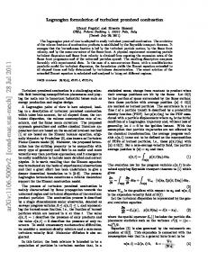
Figure 1.3: Constraints on the matter density of the universe and the cosmological constant by brightness measurements of high-redshift SN Ia. From Riess et al. (1998)

constant at a high confidence level (see figure 1.3). The value for ΩΛ is obtained from the fact that the distant SN at a redshift of about 1 are appear to be systematically dimmer by ≈ 0.25 mag as would be expected in a universe with ΩΛ = 0. Since this deviation is smaller than the intrinsic scatter of SN Ia, some caution is advised: even a small systematic error caused by incorrect assumptions may result in a significant change of the predicted Ω Λ . As a hypothetical example, the dimness of the distant SN Ia could be caused by some kind of “grey dust” with a constant absorption coefficient for all optical wavelengths, which is distributed evenly across the universe. Unless other distance indicators independent of absolute luminosities are found, there is no way to decide if this dust exists or not. The discrepancy in brightness could also be the consequence of evolution effects like a slightly different chemical composition of the progenitor stars at z ≈ 1, when the universe was considerably younger than today. Livio (2000) mentions the possibility that the SN Ia samples at low and high redshifts could be dominated by different progenitor populations (e.g. mostly sub-MCh explosions at z ≈ 1 and mostly MCh explosions today); this can happen if the pre-supernova evolution time is significantly different in the two scenarios. This idea can only be verified or falsified when all different progenitor models and their dependency on cosmological evolution have been studied in a quantitative manner. To obtain more complete information about possible evolution effects and their influence on SN Ia observables, data from redshifts of 0.1 / z / 0.5 would be very helpful. Unfortunately there is a gap in the observations at these intermediate redshifts (which is also evident in figure 1.3), because no good strategy exists for detecting them: they are too weak to be

17

1

I NTRODUCTION

AND MOTIVATION

discovered in wide-field surveys and they are not numerous enough to allow “scheduled” observations in a small sky region. A complete coverage of SN Ia from redshifts 0 to 1 is still many years away.

1.5

Goals of this work

The numerical models and simulations presented in this work are concerned with the short stage (approximately one second) of fast nuclear fusion reactions, during which the largest part of the explosion energy is released. Since one of the main goals is a better insight into the physical processes occuring during the explosion and not so much a precise fitting of particular SN Ia events, only models without free parameters were considered. As was mentioned in the beginning, the total energy release serves as a fundamental comparison criterion between simulation and observation results. Only if a set of numerical models produces energies in the correct range, it can be considered a promising description of the SN Ia explosion mechanism. Of course, other features like the ejecta composition and expansion velocities must also be reproduced by a correct model, but obtaining this information from simulations not only requires numerical treatment of the combustion phase, but also the of the remnant’s evolution over several weeks. While this kind of verification is beyond the scope of this work, additional facilities were provided in the simulation code to allow such follow-up calculations, which are planned for the near future. Once the model has been proven to produce a SN Ia-like event, the next goal is to thoroughly investigate the influence of various physical parameters, like the progenitor’s composition, accretion history and rotation profile. Varying these values within a reasonable parameter space should, for a correct model, reproduce the observed scatter in explosion strength and its correlation with the light curve shape etc. Such a discovery would give valuable insights on the physical origin of this correlation and could greatly increase the credibility of the hitherto purely empirical luminosity corrections applied for cosmological measurements. Apart from this known scatter, parameter studies might also reveal evolution effects, i.e. a dependence of the SN characteristics from the age of the universe at the time of the explosion. In this context, a correlation between the explosion strength and the chemical composition of the white dwarf – which is arguably different at high redshifts and the current time – appears most likely. Only if this possibility is ruled out, or if the correlation has been studied in detail, SN Ia can be used as “standardizable candles” and therefore as distance indicators with good conscience. The outline of this work is as follows: in the following chapter, the mathematical equations describing all processes relevant for the combustion phase are introduced. Chapter 3 discusses how the equations for the macroscopic phenomena are discretized in space and time to allow their numerical integration. The important microphysics cannot be resolved in simulations of the entire star and therefore must be described by models, which are presented and motivated in detail. Special emphasis is laid on the description of the model for the thin reaction front, since the employed numerical scheme has not been used in an

18

1.5

G OALS OF THIS WORK

astrophysical context before: chapter 4 contains a comparison of this tool with other methods currently in use, as well as an extensive discussion of the implementation details and potential difficulties. The second part of the work focuses on supernova simulations carried out with the developed code. Chapter 5 recapitulates the used equations and solution methods for quick reference and then describes the employed stellar model and grid geometry as well as a test calculation to assert the hydrostatic stability of this configuration. In the next chapter, twodimensional SN simulations are presented and discussed, whose goal is mainly to study the correctness and robustness of the numerical methods and to investigate the influence of different initial flame configurations on the explosion process. A few fully three-dimensional calculations were also performed; their results are shown in chapter 7 and compared to the two-dimensional simulations. Finally, chapter 8 summarizes the new physical insights gained, discusses advantages and shortcomings of the current approach and suggests possible future improvements. Also, the results are compared to other works in the same area, and their significance for other branches of astrophysics is briefly discussed.

19

Part I Physical and numerical background

21

2 Governing equations In this chapter the fundamental physical and mathematical concepts will be presented, which are needed to describe a SN Ia event in terms of a system of equations. First, the formulae for the treatment of an ideal fluid are introduced; those are expanded in the following sections to incorporate external forces, internal source terms and dissipation effects. Chemical or nuclear reactions within the fluid can take place in many different ways. An overview over these burning modes is given in section 2.2, including a more detailed discussion of so-called “thin flames”, i.e. combustion processes with highly temperaturedependent reaction rates and consequently very stiff source terms in energy and species concentrations. Under certain conditions the inherent nonlinear nature of the resulting set of partial differential equations results in unpredictable, chaotic behaviour of the fluid. Several different cases for this transition to turbulent flow are relevant for this work and their properties are briefly discussed, with an emphasis on turbulent burning processes.

2.1

Hydrodynamics

Throughout this work the white dwarf matter will be interpreted as a continuum. This approach is justified because the star can be subdivided into volume elements which are larger than the mean free paths of the individual particles, but at the same time much smaller than the scales on which statistically defined quantities like temperature and density change perceptibly. Furthermore all particles are in thermodynamical equilibrium on this scale, so that a single set of thermodynamical quantities completely describes the state of the material. The interpretation as a fluid is justified because the material has negligible resistance to shear. Starting from the minimal equations describing fluid flow, the extensions and generalizations required for the understanding and simulation of Type Ia SN are presented and motivated one by one.

2.1.1 Basic equations Most of the equations of hydrodynamics take the form of local conservation laws: in a given volume element, the rate of change of any volume-related quantity a is equal to the total

23

2

G OVERNING EQUATIONS

flux of that quantity over the surface of this element (neglecting explicit source terms): Z I ∂a 3 ~ = 0. d r+ a~vdA (2.1) V ∂t ∂V The surface integral in this expression can be transformed to a volume integral according to Gauss’s law, resulting in Z ∂a ~ + ∇(~va) d3 r = 0. (2.2) ∂t V In the (idealized) case of a continuum it is possible to make the transition to an infinitesimally small volume element and the integration can be omitted: ∂a ~ + ∇(~va) = 0 ∂t

(2.3)

It must be noted, however, that this differential form cannot be applied easily to flows containing jumps in one or more state variables like idealized contact discontinuities and shocks, since the derivatives will contain singularities. This class of so-called “weak solutions” is better treated by the conservation laws in integral form. The above equations can be used directly to describe the conservation of mass, which results in the continuity equation: ∂ρ ~ + ∇(~vρ) = 0 ∂t

(2.4)

The corresponding equations for the momentum components contain an additional source term, since the fluid is accelerated in the opposite direction of a pressure gradient: ∂(ρvi ) ~ ∂p + ∇(~vρvi ) = − ∂t ∂xi

(2.5)

Combination of eqs. (2.4) and (2.5) leads to the so-called Euler equation for ideal fluids without external forces: ~ ∂~v ~ v = − ∇p + (~v∇)~ (2.6) ∂t ρ Finally, the conservation law for the specific total energy etot reads ∂ρetot ~ ~ vp). + ∇(~vρetot ) = −∇(~ ∂t

(2.7)

The equations above, however, still do not completely describe the physical situation; in order to couple pressure and energy to the other state variables, a material-dependent equation of state (EOS) is required: p = fEOS (ρ, ei , X) T = fEOS (ρ, ei , X)

(2.8) (2.9)

The vector X denotes the composition of the fluid; it contains the mass fractions for the different chemical species.

24

2.1

H YDRODYNAMICS

2.1.2 Source terms In the context of this work, the minimal equations given above must be extended by several terms to account for self-gravity and thermonuclear reactions. External forces Any accumulation of matter produces a gravitational potential Φ which – in the Newtonian limit – is given by Poisson’s equation: ∆Φ = 4πGρ

(2.10)

The acceleration of the fluid by gravitation leads to a source term in the momentum and energy equations. Combustion The thermonuclear reactions during a supernova explosion change the chemical composition of the progenitor material and release a certain amount of energy. The reaction rates r are usually given as functions of ρ, T , and the composition X. The influence of the reactions on the hydrodynamics takes the form of an additional source term S in the energy equation and a set of equations for the time dependence of X. The full set of hydrodynamical equations now reads: ∂ρ ~ + ∇(~vρ) = 0 ∂t ~ ∂~v ~ v = − ∇p − ∇Φ ~ + (~v∇)~ ∂t ρ ∂(ρetot ) ~ ~ vp) − ρ~v∇Φ ~ + ρS + ∇(~vρetot ) = −∇(~ ∂t ∂(ρX) ~ + ∇(~vρX) = r ∂t r = f(ρ, T, X) p = fEOS (ρ, ei , X) T = fEOS (ρ, ei , X) S = f(r) ∆Φ = 4πGρ

(2.11) (2.12) (2.13) (2.14) (2.15) (2.16) (2.17) (2.18) (2.19)

This system is known as reactive Euler equations including gravitation.

2.1.3 Real fluids While the equations above are appropriate for numerical supernova simulations (for reasons given in section 3.1), they still only describe a so-called “ideal fluid” (or “dry water”, as it was called by John von Neumann): i.e. internal friction and diffusion are neglected. For the theoretical investigation of the supernova event, however, these effects must be taken into account, since they have an important influence on the flow behaviour on small scales and are responsible for the propagation of a flame.

25

2


Viscosity If internal friction is not neglected, the equation of motion (2.6) must be extended by an additional term describing the internal viscous forces and becomes ~ ~ ∂~v ~ v = − ∇p + fvisc . + (~v∇)~ ∂t ρ ρ

(2.20)

~fvisc must meet several constraints: it must vanish for uniform motion and for rigid rotation, ~ v = 0 and also ∇ ~ ×~v = const., and it has to be an isotropic effect. Under these i.e. if ∇~ conditions the most general expression for ~fvisc is the divergence of the tensor ∂vi ∂vj 0 ~ v) + + η 0 δij (∇~ (2.21) σij = η ∂xj ∂xi (cf. Feynman et al. 1977), where η and η 0 represent the first (or dynamic) and second viscosity coefficient. Separating this tensor into a traceless and a diagonal part yields ∂vi ∂vj 2 0 ~ v) + ζδij (∇~ ~ v), + − δij (∇~ (2.22) σij = η ∂xj ∂xi 3 where the volume viscosity ζ = η 0 + 2/3η. This form is often more convenient since it separates shear (traceless part) and bulk viscosity (diagonal part). Assuming spatially constant η and ζ, one obtains the Navier-Stokes equation for compressible fluids: h i ~ ∂~v ~ v = − ∇p + 1 η∆~v + ζ + η ∇( ~ ∇~ ~ v) . + (~v∇)~ ∂t ρ ρ 3

(2.23)

In the divergence-free case this reduces to ~ ∂~v ~ v = − ∇p + η ∆~v. + (~v∇)~ ∂t ρ ρ

(2.24)

Since the viscous momentum transport also implies an energy transport, an additional 0 /∂xj ) must be added to the right hand side of the energy equation (2.13). source term ~v(∂σij It is evident that viscosity effects transform kinetic energy into internal energy, thereby increasing the entropy of the system. In contrast to ideal flow, real flow is therefore an irreversible process. Diffusion Any temperature and composition fluctuations in a fluid tend to balance themselves out over time by heat and material diffusion. This effect becomes especially important for steep gradients and on small length scales as is the case for thin flames. In this particular situation the cold fuel is heated by energy diffusion from the burned region; at the same time fuel particles diffuse into the ashes and vice versa.

26

2.2

C OMBUSTION THEORY

These processes are described by the terms ∂ρetot ~ e ρcp ∇T ~ ) = ∇(κ ∂t ∂ρX ~ X ρ∇X). ~ = ∇(κ ∂t

and

(2.25) (2.26)

In the case of SN Ia, diffusion effects play a crucial role for the flame propagation on microscopic scales. These processes cannot be resolved in simulations covering the whole progenitor star and must therefore be replaced by a numerical model. On the macroscopic scales heat and material diffusion are unimportant, so that the equations above can be omitted in our hydrodynamic scheme.

2.2

Combustion theory

A combustion process in a fluid can be described as a temporal change of the fluid composition in combination with the release of thermal energy. Depending on quantities like diffusion cofficients, heat capacity, energy release, reaction rates, sound speed and turbulent mixing, this process will take place in vastly different regimes. If the time scale for mixing (be it by diffusion, convection or turbulence) is shorter than the reaction time scale, burning will convert fuel to ashes homogeneously in a large volume; this situation is encountered in nova outbursts, for example. High activation energies and low conductivities, on the other hand, will produce a very thin reaction layer (a flame) propagating through the fuel and leaving behind the burning products. Many intermediate and significantly distinct modes of combustion are realized in nature; in many cases (including SN Ia), turbulence has an important influence on the characteristics of the combustion. All burning processes described in this work fall into the category of premixed combustion, i.e. all ingredients necessary for the reaction are present in the fuel mixture; a chemical analogon would be a Bunsen flame. Diffusion flames, where reaction can only take place at the interface between two fuel components, do not occur in the context of SN Ia.

2.2.1 Laminar flames One of the very few combustion processes that can be treated asymptotically (Zeldovich et al. 1980) is the so-called laminar deflagration, a reaction zone propagating by diffusion at subsonic speed. In this scenario all quantities only depend on one spatial coordinate. Furthermore all time derivatives vanish in the rest frame of the deflagration front. These conditions are fulfilled for a planar flame propagating at constant speed through an infinitely large medium. Pure laminar deflagration is unlikely to occur in the real world because of boundary effects and the presence of various instabilities; nevertheless knowledge of the properties of laminar flames is a prerequisite for the investigation of turbulent combustion. One of the reasons is that the speed of a laminar flame is the lower limit for the velocity of any stationary deflagration front in a given medium.

27

2


A crude estimate for the propagation velocity sl of a laminar flame can be obtained from the following consideration (Timmes & Woosley 1992): The fuel reaches the point of ignition by heat transport and material diffusion of fuel and ashes into each other; the energy generation rate depends on the reaction rates and therefore mainly on the temperature. Since all quantities are constant in time, all the energy released in the reaction zone must be carried away by diffusion (mechanical expansion work is neglected in this approximation). This is roughly equivalent to the postulate that the burning and diffusion timescales are equal: τdiff =

ei l2F ! = τburn = . λc S

(2.27)

Here lF is the flame width, λ and c denote the mean free path and average velocity of the particles transporting the heat and S the energy generation rate in the reaction zone. The laminar flame speed can be expressed by sl = lF /τburn (Landau & Lifschitz 1991), which leads to r r λcei λcS lF = and sl = . (2.28) S ei To obtain estimates for lF and sl , typical values for ei and S must be supplied, which is a non-trivial task because of the nonlinear temperature dependence of S (Timmes & Woosley 1992). In reality the simple picture of two constant states of unburned and burned material on both sides with a reaction layer of thickness lF in between is not sufficient to explain all effects observed in combustion experiments. The flame is better described as a combination of two separate regions. The so-called preheating zone consists of fuel and contains a temperature gradient created by heat diffusion from the hot reaction products. In this region the temperature is not yet high enough to produce noticeable reaction. All the energy is generated in the adjacent reaction zone, where a runaway process takes place and the temperature rises very fast from the ignition temperature to its final value in the ashes (cf. Peters 1999). In many cases – especially for reactions with a high activation energy – the preheating zone is much wider than the reaction zone; this implies that two different length scales are needed to characterize a laminar flame (for an example see section 2.4.2).

2.2.2 Jump conditions for thin flames Any chemical or nuclear reaction takes place on a timescale τR . The width lF of the reaction zone depends on τR and on the propagation speed s. In situations where lF is much smaller than the length scales one is interested in, or lies below the resolution of a simulation, the internal structure of the flame can be neglected and it may be treated as a mathematical discontinuity. All quantities that would undergo a smooth transition from the unburned to the burned state in the reaction zone now exhibit a sharp jump at this discontinuity. Equations for these jumps are derived most conveniently in a frame of reference where the flame is at rest and the fluid velocity has only a component normal to the flame. Such a system always exists because the fluid velocity component tangential to the front must be equal on both sides; if it had a jump, tangential momentum would not be conserved if s 6= 0.

28

2.2

C OMBUSTION THEORY

front (v=0)

v1 ρ1

v2 ρ2

p1

p2

Figure 2.1: Schematic illustration of a thin flame front

In this system, the changes for mass, momentum and energy flux across the flame are given by the so-called Rankine-Hugoniot jump conditions: ρ1 v 1 = ρ 2 v 2 ρ1 v21

+ p1 =

ρ2 v22 v22

(2.29) + p2

v21 + ei1 + p1 V1 + ∆w0 = + ei2 + p2 V2 . 2 2

(2.30) (2.31)

These equations are obtained directly from the conservation laws (2.11) – (2.13), integrated over a volume element which encloses part of the front. The indices 1 and 2 refer to unburned and burned material, respectively (see also figure 2.1). The term ∆w0 is the difference of the formation enthalpies of ashes and fuel; it corresponds to the amount of energy released by the instantaneous reaction. Without loss of generality we define that a positive velocity means a movement in the direction of the fuel; the normal fluid velocities v[12] are then equal to −s[12] . In a frame of reference where the front is not at rest, only the weaker condition vn1 − vn2 = s2 − s1

(2.32)

holds. By simple transformations of the Rankine-Hugoniot conditions one can obtain more descriptive relations. Combination of eqs. (2.29) and (2.30) yields the Rayleigh criterion: p2 − p 1 = −(ρ1 v1 )2 = −(ρ2 v2 )2 (2.33) V2 − V 1 This means that the slope of the line connecting initial and final state in the (p,V) diagram is a measure for the mass flux across the front. If the velocities are eliminated by combining eqs. (2.31) and (2.33), the result is the Hugoniot curve (p1 + p2 ) ei2 − ei1 = ∆w0 − (V2 − V1 ). (2.34) 2 Using the equation of state, the internal energies can be expressed by pressure and density; this leads to another relation between p2 and V2 , depending on p1 and V1 . Figure 2.2 shows an initial state (p1 ,V1 ) and the corresponding Hugoniot curve for a given ∆w0 , on which the final state must lie. Given the fact that the line connecting both states

29

2

G OVERNING EQUATIONS p

detonations unreachable

O

A A’ p

1

O’ deflagrations V1

V

Figure 2.2: Illustration of the different combustion modes

must have a negative slope (eq. 2.33), the region between A and A’ is excluded. The remaining two areas correspond to the fundamentally different modes of flame propagation: • Above A, where the burning speed s1 is supersonic, the detonations are located. In this mode of flame propagation the unburned material is first compressed to a temporary pressure p∗ > p2 ; then the reaction sets in, increasing internal energy and temperature and lowering the pressure to p2 . • Below A’ burning propagates subsonically as a deflagration. The ignition of unburned material is caused by heat conduction instead of compression. The points O and O’ are called Chapman-Jouguet points; at these points s 2 is equal to the sound speed in the reaction products and the fuel consumption rate reaches a maximum for deflagrations resp. a minimum for detonations. In reality, detonations between O and A do not exist, because all paths in the pV-diagram describing a detonation will cross the upper detonation branch first and a transition between both branches is not possible (Landau & Lifschitz 1991). Also, fast deflagrations with a final state below O’ will only occur in very exceptional situations, because heat diffusion from ashes to fuel has to be faster than the sound speed in the burning products, which is very difficult to realize. All combustion processes investigated in this work are slow deflagrations (very close to A’ in the diagram) and therefore have the properties p1 ' p2 , s[12] c[12] and ρs2[12] p[12] .

2.3

Hydrodynamical stability and turbulence

A solution of the hydrodynamical equations is regarded as unstable if a small perturbation in the initial conditions grows exponentially, thereby leading to a completely different solution than in the unperturbed situation. As long as the differences between both solutions are sufficiently small, the growth rates of the various hydrodynamical instabilities can be

30

2.3

H YDRODYNAMICAL STABILITY

AND TURBULENCE

determined by linear stability analysis (cf. Landau & Lifschitz 1991). In this approach the exact solution is superposed with a small perturbation ~v1 (~r,t) and p1 (~r,t) in such a way that the resulting flow still obeys the equations of motion, provided that terms of higher than first order in ~v1 and p1 are neglected. The general solution for ~v1 of the resulting system contains terms of the form eωt ; therefore positive results for ω indicate that the flow is unstable in the linear regime. Nonlinear stabilization effects that prevent the perturbations from growing without limit have been observed in a few cases, but these phenomena can, in general, only be analyzed by numerical studies.

2.3.1 Relevant types of instability As was already mentioned in section 1.3.3, the thermonuclear flame in an exploding white dwarf is deformed by several instabilities on a wide range of length scales. Their dynamical behaviour will be discussed briefly in the following. Rayleigh-Taylor instability: This kind of instability always occurs when a lower-density fluid is accelerated towards higher-density material, e.g. by a gravitational field. A simple case that can be treated analytically is the layering of two different fluids 1 and 2, separated by a thin interface. In the linear approximation the growth rate of the instability is given by r ρ1 − ρ 2 (2.35) ωRT = gk ρ1 + ρ 2 (cf. Chandrasekhar 1961). Here g denotes the acceleration towards the medium 1 and k is the wave number. It is evident that perturbations will only grow if ρ 1 > ρ2 and that the growth rate is faster for smaller perturbation wavelengths. In reality, however, nonlinear effects will dominate the flow characteristics very soon, resulting in large rising bubbles of light material with fingers (in 2D) resp. rings (in 3D) of dense material sinking down in between. This pattern is caused by the fact that the rise velocity of larger buoyant structures is faster and that they will “swallow” smaller bubbles when overtaking them. In a SN Ia, the reaction products have a smaller density than the surrounding matter and rise towards the star’s surface, thereby creating a RT-unstable situation. On large scales, however, the instability is suppressed by the overall expansion of the star during the explosion. This effect becomes important at a given scale when the star expands by a significant amount during the eddy turnover time on that scale. Kelvin-Helmholtz instability: Any volume of fluid containing a shear flow is subject to this instability. Considering again a simplified situation of two regions separated by a jump ∆v in the tangential velocity, the growth rate is √ ρ 1 ρ2 ωKH = k ∆v (2.36) ρ1 + ρ 2 (cf. Landau & Lifschitz 1991). Like in the above case all wavelengths are unstable, but there is no nonlinear mechanism which suppresses small-scale features, at least

31

2

G OVERNING EQUATIONS not in this idealized situation. In real flows there will always be a shear layer of finite thickness instead of a velocity discontinuity due to viscosity; in this case, perturbations with high wave numbers will not grow. KH-instabilities will develop at the sides of RT-bubbles, where there is a rather sharp transition from rising ashes to cold fuel sinking down in between. For the special case of a discontinuity propagating through the medium (e.g. for a flame) there will be an additional stabilizing effect on small scales, because an abrupt jump of the tangential velocity at the front is prohibited by momentum conservation (see section 2.2.2) and the transition layer will be smeared out beyond the shear layer thickness.

2.3.2 Properties of turbulent flow The equation of motion for viscous fluids (2.24) does not depend individually on density, velocity, viscosity and length scale (which is represented in the equation by the spatial derivatives); substitution reveals that it only depends on a single dimensionless quantity Re (the Reynolds number), which can be defined by Re =

ρlv 0 (l) . η

(2.37)

This means that for different setups, which nevertheless are characterized by the same Reynolds number, the features of the resulting flows will be similar. In the formula above, l and v 0 (l) represent a length scale of interest and the magnitude of velocity fluctuations at this length scale; in the simple case of water flowing past a cylinder, for example, l could be the cylinder radius and v 0 (l) the fluid velocity far away from the cylinder. It is evident from this formulation that, for a given setup, Re is a monotonically increasing function of length scale and that the behaviour of the fluid will consequently vary depending on the observed scale. A large number of experiments has shown that at Reynolds numbers / 10 the flow is stationary and laminar, whereas for Re ' 200 the velocity field exhibits chaotic fluctuations in space and time, which take the form of vortices (or eddies) with different sizes. This phenomenon is called turbulence and behaves isotropically even for anisotropic initial conditions. Between those two extreme regimes stationary eddies or periodic oscillations in the flow patterns are observed. It is obvious that a certain length scale must exist for any kind of turbulence below which the flow will be essentially laminar. This scale lk (the Kolmogorov scale) is defined as Re(lk ) ≈ 1.

(2.38)

Richardson (1922) interpreted these results as a turbulent energy cascade: eddies of a given size will decay into smaller ones with a lower rotation velocity, until lk is reached. At this scale the eddies are slowed down by viscosity and their kinetic energy is transformed into heat. For turbulent flow, which is stationary in a statistical sense, the rate at which energy is transported from larger to smaller scales must be independent of the scale and has to be

32

2.3

H YDRODYNAMICAL STABILITY

AND TURBULENCE

equal to the dissipation rate ε of kinetic into thermal energy at lk , otherwise the energy at a given scale would change with time. Clearly, a well defined scale lk where all of the turbulent velocity fluctuations are abruptly dissipated is an idealized concept; in reality the influence of viscosity will gradually increase for smaller and smaller scales, until the turbulent motions have been damped completely. Also, if the turbulence is driven at a scale ld , isotropic turbulent flow can only be expected at length scales which are considerably smaller than ld . Therefore the range of scale space where isotropic, inviscid turbulence can be observed is limited to the so-called inertial range, where lk l l d . (2.39) An expression for ε can be determined by dimensional analysis: since it is equal to the energy transfer rate from larger to smaller scales in the inertial range, it must be proportional to a combination of the quantities describing the flow in that range, namely ρ, l and v 0 (l). The only combination with the desired unit of erg g−1 s−1 leads to the expression ε∝

v 0 (l)3 . l

(2.40)

In order to determine the spectrum of v 0 (l) one makes use of the fact that the Navier-Stokes equation is invariant with respect to the scaling transformation ~r? := λ~r, ~v? := λh~v, t? := λ1−h t;

0 0 in the ashes. ~ to the interface is needed. We define it to During the following discussion the normal n point towards the unburned region, resulting in ~ =− n

~ ∇G . ~ |∇G|

(4.5)

4.1.2 Temporal evolution For the implicitly given Γ the differential equation for the time evolution is not as obvious as for the marker-string method. However, the desired expression can be determined by the following consideration:

53

4

T HE LEVEL

SET METHOD

Let P be an imaginary point attached to the flame surface. The movement of P in an Eulerian frame of reference (named ~x˙ P ) then consists of two contributions: the advection by the fluid motions and a propagation term in normal direction caused by the burning itself. Since the fluid velocity has a discontinuity at the front and the burning velocity is different at the burned and unburned side (eq. 2.32), both quantities must be taken from the same side of the front. The result is identical for both sides; traditionally, the unburned quantities (index 1) are chosen: ~x˙ p = ~v1 + s1 n ~ (4.6) Because P is attached to the front, and thereby to the zero level set of G, the value of G(~xP ) cannot change with time: ∂G ~ dG(~xP ) = + ∇G · ~x˙ p := 0, dt ∂t

(4.7)

which together with eqs. (4.5) and (4.6) leads to the desired differential equation for the time dependence of G: ∂G ~ = −(~v1 + s1 n ~ ~ ~ )(−~ ~ + s1 )|∇G| = −~x˙ p ∇G n|∇G|) = (~v1 n ∂t

(4.8)

Of course this derivation is only valid for points lying on the front; in other places the concept of front motion (~x˙ p ) makes no sense and the required velocities might not even be defined. This means that another prescription for ∂G/∂t has to be chosen in the burned and unburned regions, or that the propagation speed is extended into those regions according to some prescription. In principle there are no constraints on the shape of G in these areas, since only the zero ~ ~ and ∇G level set is needed for the flame model. However, the appearance of the terms n in equation (4.8) is a strong hint that G should be a smooth function with a well-defined gradient in order to avoid numerical difficulties when working on discretized problems. This rules out the fairly obvious choice of the step function    1 in the burned region G = −1 in the unburned region (4.9)   0 at the front,

whose disadvantages are discussed by Mulder et al. (1992). For our purpose it is a good choice to postulate that G is a distance function, i.e. that ~ ≡ 1, |∇G|

(4.10)

with the exception of singular points like extrema of G. This prescription ensures a numerically well-behaved level set function. To obtain numerical stability, however, it need not be ~ does not deviate much from 1 and does not change fulfilled exactly: it is sufficient that |∇G| abruptly in space. A sample of an interface in two dimensions and the resulting level set function is shown in figure 4.2.

54

4.1

I MPLICIT

DESCRIPTION OF PROPAGATING INTERFACES

Figure 4.2: Illustration of a signed distance function G constructed from a closed curve in two dimensions (black line).

4.1.3 Re-Initialization Several different algorithms have been developed to solve equation (4.10). Sussman et al. (1994) employ a pseudo-time method and iterate the expression ∂G G ~ 1 − |∇G| (4.11) = ∂τ |G| + ε

~ = 1 is obtained. Here, the pseudo-time step ∆τ ≈ 0.1∆ and ε ≈ ∆, until convergence to |∇G| where ∆ is the dimension of the smallest grid cell. To preserve the G-values near the front ~ at a given point is always evaluated in the direction of ∇G ~ for G < 0 it is crucial that |∇G| ~ for G > 0; this way, information can only flow from the front outwards and the and −∇G zero level set itself is disturbed as little as possible. This procedure is rather easy to implement and only relies on local data, which allows efficient execution on distributed memory machines. Unfortunately the front tends to shift by small amounts during the re-initialization because of the finite cell size; this effect (illustrated in figure 4.3) disturbs the simulation outcome, especially for slowly moving flames. The problem can be alleviated by introducing a weighting function to ∂G/∂τ that suppresses changes of G at small distances d from the front. In this work, the function −d0 d − d0 . 1 − tanh (4.12) H(d) = 1 − tanh δ/3 δ/3

was chosen (R. Klein, personal communication). Since d is not known a priori and G is itself an approximate signed distance function, it seems appropriate to substitute d by |G| in the equation above. This function then results in a smooth transition from suppression to full application of the correction in a region from d0 − δ < |G| < d0 + δ. A value of d0 = 3∆ and δ = ∆ was used for the presented simulations.

55

T HE LEVEL

SET METHOD

correction

4

co rre ct ed

unphysical front motion

i

inal

orig

G

i+1

i+1

correction

Gi

Figure 4.3: Unphysical shifting of the front during re-initialization according to Sussman et al. (1994), shown for a 1D case. The (exaggerated) correction of the gradient in the cell containing the front will move the root of G.

A further refinement of the method is required to obtain a correct distance function in the presence of topological changes of the flame geometry. Figure 4.4 depicts a onedimensional situation where two burned regions have merged in the last flame propagation step. In the neighbourhood of this event the values for |G| are obviously still very small, despite the fact that the front is now quite far away. The re-initialization algorithm described so far will not change these values, since a small |G| is interpreted as being close to the front. For proper algorithm behaviour it is therefore necessary to find a better estimate of the front distance. We use the following approach, which is reasonably efficient and local: Since the full correction has to be applied in all cells with a distance ≥ d0 + δ from the front, it is sufficient to determine a distance guess only for cells lying in a narrow band around the front. For this purpose the coordinates of all roots of G on the grid cell edges are calculated in linear approximation; this set of points represents a crude discretization of the zero level set. Now for all cells in the vicinity of the front the minmum distance to any of these points is calculated; this value then serves as the distance guess d in eq. (4.12). The reinitialization method described here has a complexity of O(N 3 ( δ0∆+δ )3 ) for a grid consisting of N3 cells. A different approach to maintain the distance function property of G is to perform no reinitialization step at all, but to construct a so-called extension velocity field on the computa~ unchanged during propagation. It is particularly useful in tional domain, which leaves |∇G| situations where the propagation speed is only defined at the location of the front itself and has no physical meaning elsewhere (e.g. when simulating crystal growth). The extension ~ in the cells cut by the front and obeys the velocity is perpendicular to G, equals s1 + ~v1 n condition ~ ext ∇G ~ =0 ∇v (4.13) everywhere else. An efficient algorithm for constructing vext is given in Adalsteinsson & Sethian (1999). This method is non-iterative and does not change the G-values near the front directly; however, a straightforward implementation on a parallel computer requires

56

4.1

I MPLICIT

DESCRIPTION OF PROPAGATING INTERFACES

G

burned

unburned

x

Figure 4.4: Form of the G-function shortly after the merging of two burned regions. The portion of G inside the dashed circle will not be re-initialized properly.

an excessive amount of inter-process communication and is therefore rather slow, despite the low complexity of O(N3 log N). Finding an optimized parallel algorithm for the creation of extension velocities should have high priority in the further development of the supernova code.

4.1.4 Complete Flame/Flow-Coupling Throughout the last section the knowledge of ~v1 and s1 was assumed without mentioning in the cells cut by the front. However, these quantities cannot be determined, unless the treatment of the discretized Euler equations, which was described in section 3.1, is refined to take the existence of a discontinuity at the front into account. Without additional measures the transition between pre- and post-front states will be smeared out over a few cells, such that the exact states in the vicinity of the front cannot be reconstructed. For an accurate treatment of the coupling between the flame and the surrounding flow it is necessary to implement in-cell reconstruction and flux splitting as described by Smiljanovski et al. (1997). In this approach a grid cell can be either completely burned, completely unburned or mixed; in the latter case its state is a well defined linear combination of burned and unburned states: ρ¯ = αρ1 + (1 − α)ρ2 ρ¯e¯tot = αρ1 etot,1 + (1 − α)ρ2 etot,2 ρ¯~v¯ = αρ1~v1 + (1 − α)ρ2~v2

(4.14) (4.15) (4.16)

The parameter α denotes the volume fraction occupied by the unburned state. Since the tangential velocity component must not change across the front, it is convenient to separate the fluid velocities into two parts ~ vn := ~vn

~, and ~vt := ~v − vn n

(4.17)

resulting in the simpler equations ¯vn = αρ1 vn1 + (1 − α)ρ2 vn2 ρ¯

and ~vt1 = ~vt2 = ~v¯t .

(4.18)

57

4

T HE LEVEL

SET METHOD

F2 F1

β

α

F2 F1

F2

F2

Figure 4.5: In-cell reconstruction and flux splitting allow complete separation of burned and unburned states.

Additional relations are obtained from the jump conditions across the flame: p2 − p 1 V2 − V 1 (p1 + p2 ) (V2 − V1 ) ei2 − ei1 = ∆w0 − 2 ρ1 vn2 − vn1 = s1 1 − ρ2 (ρ1 s1 )2 = −

(4.19) (4.20) (4.21)

Together with the equation of state p1 = pEOS (ρ1 , ei1 , X1 ) and p2 = pEOS (ρ2 , ei2 , X2 )

(4.22)

and the burning speed law s1 = max

p

2q, sl (ρ1 )

(4.23)

it is possible to reconstruct the states 1 and 2 for a given mixed state. To ensure that no burned material can enter an unburned cell and vice versa by numerical diffusion, the fluxes between mixed cells and their neighbours must be computed separately for fuel and ashes. After the Riemann problem has been solved for both components, the total flux across a cell interface is calculated according to the linear combination F¯= βF1 + (1 − β)F2 ,

(4.24)

where β is the fraction of the cell interface occupied by the unburned state and the vector F contains the fluxes of mass, momentum, energy and species. This flux splitting technique is illustrated in figure 4.5.

4.2

Implementation details

4.2.1 Level set propagation The complete coupling approach has been implemented successfully for various applications (see, e.g., Smiljanovski et al. 1997). However in the case of SN Ia simulations a combination of numerical obstacles that is not present in these other works has so far prevented its use. An obvious point is that the reconstruction equations require the existence

58

4.2

I MPLEMENTATION

−

+ −

+

+

− +

−

DETAILS

Figure 4.6: Discretization problems in two dimensions: for alternating signs of G the location of the front and therefore the unburned cell fraction α is ambiguous. Furthermore the presence of two fronts propagating in nearly opposite directions cannot be described by a single normal vector.

−

−

+

+ −

+

− +

Figure 4.7: In three dimensions the roots of G on the cell edges do not necessarily lie on a plane.

~ in every mixed cell, which implies that the front is approximated of a single front normal n by a straight line or a plane. While this is reasonable for nearly straight flames, it is not clear how to deal with a very convoluted front geometry, where more than one flame segment can exist in a single cell (see figure 4.6). The situation is even more problematic in three dimensions, because it is not generally possible to describe a contiguous surface with only one planar polygon per grid cell, even if only one flame section exists per cell (figure ~ , there will 4.7). Whatever approach is taken to overcome these difficulties and determine n always be an inconsistency between this normal and the unburned cell fraction α, which in turn causes inaccurate results for the reconstructed hydrodynamical quantities. It has been shown by Reinecke et al. (1999b) that in degenerate white dwarf matter even small inaccuracies of the input parameters can cause the reconstruction algorithm to fail, because no physically meaningful solution exists. This sensitivity is a consequence of the equation of state, which exhibits rather extreme behaviour at low temperatures, e.g. ∂T lim = ∞. (4.25) T →0 ∂e ρ Since such terms are present in the Jacobian matrix of the reconstruction equation system, small errors in the input can have a dramatic impact on the results. This difficulty is not

59

4

T HE LEVEL

SET METHOD

encountered in simulations of ideal gases since their equation of state is much more wellbehaved. As a consequence of these problems a different approach was adopted for the propagation of the flame, which does not require the reconstructed velocity ~v1 of the unburned material but uses the averaged velocity in the cell instead. While this is in general a very bad approximation, it can be justified in our case for two reasons: • The density jump across the flame is not very high (ρ2 /ρ1 ' 0.5 throughout the whole explosion). As a consequence, the velocity difference |~v¯− ~v1 | is smaller than the burning speed s1 (eqs. 2.29 and 2.32). This is only a very small fraction of the typical fluid speeds during the explosion. • The turbulent burning speed is derived from dimensional analysis and only determined up to a factor near 1 anyway. Any deviations from the assumed value caused by the simplified level set approach are smaller than this inherent uncertainty in our case. It is convenient to split the propagation of G into an advection and a combustion part. Mulder et al. (1992) pointed out that the advection by an underlying flow field can be formulated in a conservative manner, yielding Z

V

∂(ρG) 3 d r+ ∂t

I

~ = 0. ~vfluid ρGdA

(4.26)

∂V

This expression is identical to the advection equation of a passive scalar; therefore this part of the time evolution of G can be performed by the PPM algorithms already present in the code. The front motion due to burning was calculated in a separate step according to the formula

∂G ∂t

burn

~ = s|∇G|,

(4.27)

~ is the gradient taken in the where s is the burning speed determined by eq. (3.19) and ∇G direction of steepest increase of G.

4.2.2 Re-Initialization The currently employed algorithm for the smoothing of the level set function is a variant of Sussman’s iterative method which includes all the necessary refinements discussed in section 4.1.3. It uses a pseudo time step of ∆τ = 0.1∆min , where ∆min is the smallest cell dimension of the grid. The re-initialization routine is invoked at the end of every time step ~ ≤ 4 everywhere on the grid or a maximum of 20 and is repeated until either 0.5 ≤ |∇G| iterations is reached. Though this procedure does not lead to a true distance function, it generates a sufficiently smooth G and is computationally affordable even on very unevenly spaced grids.

60

4.2

I MPLEMENTATION

DETAILS

4.2.3 Energy generation In a full implementation of the level set model the concentration changes by thermonuclear or chemical reactions per time step in every cell are given by ∆Xash = −∆Xfuel =

s1 ρ1 Afront ∆t ρ¯

(4.28)

and the corresponding energy release is ∆e = ∆Xash ∆w0 .

(4.29)

Since no reconstruction can be performed because of the reasons given in the previous section, the value of ρ1 is not known and the update of composition and energy must be done in a different way: First, an approximation of the unburned volume fraction α is calculated. Depending on the dimensionality of the simulation, two different algorithms are used: • In two dimensions, the values of G at the cell corners are obtained by linear interpolation from the cell-centered data. Then the roots of G on the cell edges are determined; the front is assumed to be the straight line between those points. The unburned area fraction can be calculated uniquely for such a configuration, with the exception shown in figure 4.6. In this special case the average of the two possible solutions is adopted as α. • In three-dimensionalp cells, the cell-centered value for G is compared to the average 3 ¯ cell dimension ∆ := ∆x ∆y ∆z :   1 α= 0   ¯ 0.5(1 + G/∆)

for G < −∆¯ for G > ∆¯ otherwise

(4.30)

The compositions and energy are then updated according to the following prescriptions: 0 Xash = max(1 − α, Xash ) 0 0 Xfuel = 1 − Xash 0 0 etot = etot + (Xash − Xash )∆w0 .

(4.31) (4.32) (4.33)

Here the exact composition of the ashes and consequently the magnitude of ∆w 0 depend on the material density (see section 3.3). This technique ensures that the material in regions behind the front is completely burned. It is not true, however, that only fuel is found ahead of the flame; since flux-splitting is not applied in our approach, the diffusion of ashes into unburned regions cannot be totally suppressed. Nevertheless this is only a minor effect because of the very low numerical diffusivity of the PPM algorithm.

61

Part II Simulations of Type Ia Supernovae

63

5 Simulation setup 5.1

Summary of the employed models

All numerical models are based on the equation system (2.11) – (2.19). The transport equations for mass, momentum, energy and species (eqs. 2.11 – 2.14) are solved in conservation form by means of the PPM algorithm described in section 3.1; for a more detailed description of the particular implementation see Fryxell et al. (1989). No artificial viscosity was used and physical viscosity and diffusion effects were neglected. The time step was determined by the CFL criterion (eqs. 3.1 and 3.2) and multiplied by a factor of 0.8 to ensure numerical stability of the PPM method. As a link between density, pressure, internal energy and composition the equation of state discussed in section 3.2 was used. Self-gravity was implemented in an approximate manner by assuming spherical symmetry of the density distribution and numerical integration of eq. (3.14) in section 3.4. The source term r in equation (2.14) consists of two independent contributions: first, all material crossing the flame is converted immediately into ash, whose composition depends on the local density ahead of the front; this part is implemented according to eqs. (4.31) and (4.32). Second, the mass ratio of α-particles and nickel in the burned region is a function of density and temperature and therefore changes during the white dwarf’s expansion (see section 3.3). Once the composition changes have been determined, the energy source term S (eq. 2.13) is obtained easily by calculating the change in nuclear binding energies from the old to the new composition. The flame geometry, which is needed to determine the stiff source terms described above, is modeled by a level set function, which is propagated and smoothed according to the procedure outlined in sections 4.2.1 and 4.2.2. For the time evolution of the level set, the flame propagation speed must be known. This quantity is determined from the laminar burning speed (eq. 3.15) and the model for the sub-grid velocity fluctuations presented in section 3.5.2, according to equation (3.19).

5.2

White dwarf model

All simulations presented in this work start out with a white dwarf of nearly Chandrasekhar mass in hydrostatic equilibrium. This implies that the differential equation Zr M0 (r)ρ0 (r) dp0 2 = −G , where M0 (r) = 4πr 0 ρ0 (r 0 )dr 0 (5.1) dr r2 0 65

5

S IMULATION SETUP Density

1010

Pressure

1030

1025 ρ [g/cm3]

p [dyn/cm2]

105

100

1020

1015

10-5 0

5.0•107

1.0•108 r [cm]

1.5•108

2.0•108

1010 0

5.0•107

1.0•108 r [cm]

1.5•108

2.0•108

Figure 5.1: Initial density and pressure profiles of the white dwarf (logarithmic scale).

holds. If a temperature distribution T0 (r) and a composition X0 (r) is prescribed, p0 and ρ0 are connected via the equation of state and this equation can be integrated straightforwardly. For all simulations, T0 = 5 · 105 K and X12 C = X16 O = 0.5 was chosen. Additionally, the central density ρ0 (0) was set to 2.9·109 g/cm3 . The resulting pressure and density profiles are shown in figure 5.1. The integration was stopped at a density of 10−3 g/cm3 ; for larger radii the density was kept constant at this value. This had to be done because of the limited range of the EOS tables (see section 3.2). It is obvious that the outer regions of the computational grid cannot be in hydrostatic equilibrium and will start to fall down onto the star’s “surface” under these circumstances; however, this has very little impact on the explosion itself, since the mass in those regions is very small (< 10−10 M ). Overall, this procedure resulted in a white dwarf mass of 2.797 · 10 33 g (slightly below MCh ) and a total energy of −5.19·1050 erg. The initial sub-grid energy level was set to q = 1012 erg/g, corresponding to turbulent velocity fluctuations of about 1.4·106 cm/s on the grid scale. This is a bit slower than the speed presently assumed for typical convective motions in a white dwarf before explosion (S. Woosley, personal communication), but according to the observations of Niemeyer & Hillebrandt (1995a) the large-eddy model tends to adapt itself to the macroscopic flow on a very short time scale (≈ 10−2 s), so that the initial value for q becomes largely irrelevant. In any case the prescription of turbulent kinetic energy on unresolved scales is somewhat inconsistent with the fact that the initial fluid velocities ~v were set to 0 on the whole grid, but constructing a macroscopic convective flow inside the white dwarf without disturbing the delicate hydrostatic equilibrium is very difficult. Anyway, the influence of such a flow field on the simulation can safely be neglected, because the rise velocities of the burned material exceed the convection already after a few time steps. The adopted setup is very similar to that of the simulations presented in Niemeyer & Hillebrandt (1995a) and Reinecke et al. (1999a) and therefore allows direct comparison of the results.

66

5.3

G RID GEOMETRY

One might argue that the model presented here is unrealistic in various respects, most notably concerning the uniform temperature and composition. In reality the star will not be isothermal, but its temperature will increase towards the surface because of accretion heating, and small temperature fluctuations will be present near the center. However, the initial temperature has no direct influence on the hydrodynamics because of the matter degeneracy; its exact value only matters for the nuclear reaction rates, which are not directly used in our flame model. A similar consideration holds for the chemical composition: while the laminar flame speed depends quite sensitively on the C/O ratio of the fuel, the macroscopic turbulent speed is practically unaffected by composition changes. On the other hand, the difference in the nuclear binding energy between carbon and oxygen cannot be neglected, so that changing the initial composition of otherwise identical progenitors might well result in significantly different explosions. This effect is not addressed here and should be subject of further study.

5.3

Grid geometry

All two-dimensional simulations were performed on a (r,z)-grid in cylindrical coordinates with the white dwarf’s center located at the origin. This arrangement imposes an artificial axial symmetry around the z-axis, i.e. all features observed in the two calculated dimensions actually represent toroidal structures around the polar axis. Additionally, equatorial symmetry was introduced by using reflecting boundary conditions along the r-axis. Consequently, only the quadrant [0;R]2 had to be calculated, with a suitably large R (see below). In three dimensions the calculations were performed on a Cartesian grid with reflecting inner boundary conditions, corresponding to an eightfold planar symmetry of the explosion. Only the region [0;R]3 was calculated. Transparent boundary conditions were applied at the outer borders in all simulations, so that material could flow freely across without unwanted reflections. Cylindrical resp. Cartesian geometry was chosen mainly because the more natural choice of spherical (r,ϑ,ϕ)-coordinates (used, for example, by Niemeyer & Hillebrandt 1995a) results in very narrow, wedge-shaped cells near the star’s center and limits the CFL timestep to rather small values. Also, the implementation of the level set and sub-grid models would have been much more delicate on a spherical grid compared to a rectangular one. Since the star expands rapidly during the explosion, parts of it will sooner or later flow across the outer grid boundaries. This is undesirable for various reasons: mass and total energy are no longer conserved, and burning processes in these outer layers cannot be accounted for. On the other hand it is not possible to enlarge the computational domain without sacrificing spatial resolution, since this would dramatically increase the required computing resources. As a compromise, Niemeyer’s approach (Niemeyer & Hillebrandt 1995a) was adopted, which consists of using a relatively fine equidistant grid in the inner regions and increasing the cell dimensions exponentially in the outer parts (see figure 5.2). In combination with the chosen coordinate systems this has the unfortunate consequence of producing very elongated, anisotropic cells near the coordinate axes, so that the sub-grid model (section 3.5.2)

67

5

S IMULATION SETUP

5.0•108

z [cm]

4.0•108

3.0•108

2.0•108

1.0•108

0 0

1.0•108

2.0•108

3.0•108 r [cm]

4.0•108

5.0•108

Figure 5.2: Illustration of the 2D grid geometry, including the initial white dwarf radius

and algorithms like the determination of α (section 4.2.3) or the level set re-initialisation (section 4.2.2) are not very accurate and somewhat inefficient. For the discussion of a probably better approach see section 8.3. Using this kind of grid, the energetically important first stages of thermonuclear burning are well resolved, and the prescription of relatively small features in the initial flame geometry is possible. When the flame reaches the anisotropic grid regions in the later phases, the pre-front density will already be quite low, so that the total amount of energy released there is small compared to the explosion energy.

5.4

Hydrostatic stability

Since the time τsim ≈ 1.5 s covered by the supernova simulations is considerably longer than the sound crossing time τsc ≈ 0.1 s of the star, it is important to test whether the initial configuration is stable over a time scale τsim when no combustion takes place. To verify this behaviour, the evolution of the white dwarf on a three-dimensional grid with a resolution of 106 cm was followed for one second. The time evolution of the star’s total kinetic energy is shown in figure 5.3. Obviously the equilibrium is not exactly realized, but the energy values are far too small to cause significant bulk expansion or contraction during the explosion: if the kinetic energy were distributed evenly over the mass of the star, the matter would only move at roughly 10 6 cm/s and therefore the internal structure of the white dwarf would not change significantly on a time scale of seconds. Furthermore the time evolution of the kinetic energy suggests that the star pulsates with a period of approximately two seconds, so that even for longer times no dramatic change (like, e.g., a collapse) has to be expected. This consideration is of course global and does not allow any conclusions concerning the movements in small regions of the white dwarf. This issue is addressed in figure 5.4, which shows a radial distribution of the maximum absolute velocity observed during the entire

68

5.4

H YDROSTATIC

STABILITY

Model stab_3d_256, kinetic energy 12

Ekin [1045erg]

10 8 6 4 2 0 0.0

0.2

0.4

0.6

0.8

1.0

t [s]

Figure 5.3: Evolution of the total kinetic energy for a simulation without thermonuclear burning. The maximum values reached in this experiment are orders of magnitude smaller than the kinetic energies expected in an exploding white dwarf.

Stability test, maximum velocities

2.0•107

|v|max [cm/s]

1.5•107

1.0•107

5.0•106

0 0

5.0•107

1.0•108 r [cm]

1.5•108

2.0•108

Figure 5.4: Radial distribution of the highest absolute material velocities reached during the entire stability test. Inside the star all velocities stay below 1.2·107 cm/s.

69

5

S IMULATION SETUP

simulation. As expected, the highest velocities are found near the surface, where density and pressure change significantly from one cell to the next, whereas there is practically no movement in the central region. In the space surrounding the star there is no pressure gradient to compensate the acceleration by gravity, which leads to high infall velocities; but since the matter density is negligible there, this has no impact on the simulation. It has to be expected that a similar test in two dimensions or more highly resolved calculations are at least as stable as the discussed case, since in both cases the discretization errors are smaller. Except for model c3_2d_128 (see section 6.2), whose results are doubtful for other reasons anyway, all presented simulations were carried out with a grid resolution equal to or higher than in this stability test. Therefore it can be assumed that numerical instability of the initial white dwarf model does not have a noticeable impact on their results.

5.5

Tracer particle distribution

To allow for post-processing, a total of 1000 tracer particles were distributed over the calculated volume in the three-dimensional calculations. The particles were arranged in a 10×10×10 grid equidistant in the integrated mass M0 (r), the azimuthal angle ϕ and cos ϑ, so that they all represent the same amount of mass. After numerical inversion of the function M0 (r), these (M, ϕ, ϑ)-coordinates are trivially mapped onto the Cartesian grid. For the two-dimensional simulations, 100 particles were distributed in r- and ϑ-direction, using the same procedure as above. Roughly once per millisecond of simulated time the location, temperature and density of the tracers is recorded; this allows accurate reconstruction of the trajectories and final velocities as well as providing the thermodynamical data necessary for detailed nuclear reaction calculations. Both results together are sufficient to construct a composition distribution in velocity space, which can again be used as input for radiation transport simulations of the later SN phases. This work does not present or discuss any results based on the tracer particle mechanism, since no post-processing with other programs has been performed up to now and therefore the additional information contained in the tracers is not yet accessible.

70

6 Parameter studies in two dimensions The goal of this chapter is to investigate the influence of physically motivated input parameters like the initial front geometry on the supernova explosion dynamics, and to verify that variations of parameters without direct physical relevance (e.g. numerical resolution) do not affect the results significantly. Because of the large number of simulations needed for such studies and the enormous computing and storage requirements, they had to be performed in two dimensions assuming axisymmetry instead of solving the full problem. Nevertheless, the insights gained from these experiments can – at least in a qualitative manner – also be applied to the three-dimensional case.

6.1

Influence of the initial flame location

As long as the secular evolution of the white dwarf before the thermonuclear runaway remains mostly unexplored, only very crude constraints can be put on the flame geometry at the onset of fast burning. Although it appears likely that the deflagration sets in at the surface of hot, floating bubbles, neither their number nor their size and radial distribution is known. Central ignition is another possible scenario that has been investigated during the last years using multidimensional calculations (Niemeyer & Hillebrandt 1995b, Khokhlov 1995, 2000); it is especially important for comparison with one-dimensional models, where off-center ignition is generally impossible (except for ignition of a spherical shell, which seems rather unrealistic). In this work the goal is to explore the corners of the large parameter space with a few quite different initial setups; once our knowledge of the pre-ignition conditions has improved due to theoretical considerations or numerical simulations, more detailed and systematic parameter studies will become feasible. The only assumption made when constructing the initial conditions was that ignition will take place within 300 km of the star’s center; this is in agreement with the findings of Garcia-Senz & Woosley (1995).

6.1.1 Choice of initial conditions Figure 6.1 shows the different setups used for the two-dimensional calculations. The flame geometries c1_2d and c3_2d represent the centrally ignited scenarios; instead of incinerating an exactly spherical region, a strong sinusoidal perturbation was applied to the front,

71

6

PARAMETER STUDIES IN

TWO DIMENSIONS

Initial condition c1_2d

3•107

Initial condition c3_2d

3•107

z [cm]

2•107

z [cm]

2•107

1•107

1•107

0 0

1•107 2•107 r [cm]

0

3•107

0

Initial condition b1_2d

3•107

3•107

Initial condition b5_2d

3•107

z [cm]

2•107

z [cm]

2•107

1•107 2•107 r [cm]

1•107

1•107

0 0

1•107 2•107 r [cm]

3•107

0 0

1•107 2•107 r [cm]

3•107

Figure 6.1: Initial flame geometries used in the two-dimensional simulations. The center of the white dwarf is located at the lower left corner.

described by the following expression: p

r 7 6 −1 z 2 2 Γ= r + z − 1.5·10 cm + 3·10 cm cos 4n tan =0 z r

(6.1)

The number of perturbations, n, was set to 1 and 3 for the geometries c1_2d and c3_2d, respectively. The rather large initially burned volume and the strong perturbation were chosen to avoid a quite long period of linear instability growth at the beginning of the explosion, during which the flame propagates slowly and not much energy is released. On the other hand it could be argued that this setup already artificially prescribes the number of large scale features that will develop during the calculation and that it might be preferable to start with a practically spherical flame, so that RT features could form at the most unstable wavelength. This objection is well founded, but to ensure that the evolution of the first small instabilities is physical and not dominated by grid artifacts would require a considerably higher resolution; this task could be subject of future studies. The off-center ignition case is represented by the setups b1_2d and b5_2d, where one and five burning bubbles were placed at at distance of about 200 km from the center. Their rather large initial size is dictated by the grid resolution: since the RT instability causes a strong deformation and elongation of the burned region, its thickness would drop below ∆ for smaller bubbles and significant parts of the flame could vanish from the grid.

72

6.1

I NFLUENCE

OF THE INITIAL FLAME LOCATION

As in the case of the white dwarf model, these flame geometries are identical to the ones discussed in Reinecke et al. (1999a); this facilitates the direct comparison of the results and the assessment of the implementation changes that were applied to various models. Although the term “bubbles” was used throughout the description above, it must be kept in mind that, due to the assumption of axisymmetry, all features in figure 6.1 actually represent toroidal structures around the z-axis. Mainly for this reason the initial symmetry of all models with respect to the diagonal is lost in the early explosion stages.

6.1.2 Explosion characteristics The time evolution of the different initial conditions, carried out on 256 2 grid cells at a central resolution of 106 cm, is shown in figures 6.2 – 6.4. The first two figures directly compare flame geometry and flow field of the central and off-center ignition conditions at different times; as an additional measure for the expansion of the star, the central density is noted in every plot. Since the initial front perturbation in the centrally ignited models is already well in the nonlinear regime, the formation of bubble- or mushroom-shaped Rayleigh-Taylor structures takes place during the first few tenths of a second. A large fraction of the burned material begins to float towards the surface, whereas the denser fuel sinks down in between. However, because of the forced axial symmetry and assumed equatorial symmetry of the model, the normal velocity component at the axes vanishes and therefore the ashes can never fully detach from the star’s center. During the evolution of model c1_2d_256 this results in a long, thin thread of burned material connecting the rising bubble with the central region. This is clearly an artifact, since in reality the initial distortion of the front will never exhibit this kind of symmetry; much more likely the burning region will float in the direction of its initially largest radial extent, and the resulting flow field will soon drive all ashes out of the center (Bychkov & Liberman 1997). A related phenomenon also occurs in the offcenter-ignition models: here, only very narrow channels exist for the backflow of fuel between the flame and the coordinate axes. The resulting, unnaturally strong shear flow causes fingers of processed material to stay near the center; this effect is clearly visible for model b1_2d_256. In a three-dimensional simulation of the whole star no such features are expected. The plots clearly exhibit strong shear flows at the sides of the rising structures, which lead to high sub-grid energy levels and thereby increase the local flame speed. In the late explosion stages the growth of macroscopic Kelvin-Helmholtz instabilities can be observed in these regions; they are most prominent in the models b1_2d_256 and b5_2d_256. In all simulations the initial symmetry is lost in a very early stage, as it was predicted above. In the case of model b5_2d_256 it is interesting to note that the individual bubbles do not stay separated during the explosion, but merge after a short time. This effect cannot be explained in the simplified picture of rising spherical bubbles whose radial growth is equal to the flame speed; in such a situation, the initial separation has to be much smaller to allow merging within less than a second. Apparently, the bubbles close to the center experience an additional radial acceleration in the wake of the bubbles at larger radii. Consequently they

73

6


4.0•107

TWO DIMENSIONS

Model c1_2d_256, t=0.30s, ρc= 1.95e+09g/cm3

4.0•107

3.0•107

z [cm]

z [cm]

3.0•107

2.0•107

1.0•107

2.0•107

1.0•107

0 0 3.16e+08cm/s

1.0•107

2.0•107 r [cm]

3.0•107

0

4.0•107

0 2.29e+08cm/s

1.4•108

1.4•108

1.2•108

1.2•108

1.0•108

1.0•108

8.0•107

8.0•107

6.0•107

6.0•107

4.0•107

4.0•107

2.0•107

2.0•107

0

0

0 2.0•107 4.0•107 6.0•107 8.0•107 1.0•108 1.2•108 1.4•108 r [cm] 5.81e+08cm/s

2.5•108

2.0•108

2.0•108 z [cm]

z [cm]

3.0•108

2.5•108

1.0•108

5.0•107

5.0•107

0 5.0•107 7.78e+08cm/s

1.0•108

1.5•108 r [cm]

2.0•108

2.5•108

3.0•108

3.0•107

4.0•107


1.5•108

1.0•108

0

2.0•107 r [cm]

0 2.0•107 4.0•107 6.0•107 8.0•107 1.0•108 1.2•108 1.4•108 r [cm] 4.96e+08cm/s


1.5•108

1.0•107


z [cm]

z [cm]


3.0•108


0

0 5.0•107 6.42e+08cm/s

1.0•108

1.5•108 r [cm]

2.0•108

2.5•108

3.0•108

Figure 6.2: Temporal evolution of the flame geometry and velocity field for the central ignition scenarios (left: model c1_2d_256, right: model c3_2d_256)

74

6.1

Model b1_2d_256, t=0.30s, ρc= 2.22e+09g/cm3

7.0•107

6.0•107

6.0•107

5.0•107

5.0•107

4.0•107

4.0•107

z [cm]

z [cm]

7.0•107

I NFLUENCE

3.0•107

2.0•107

1.0•107

1.0•107

0

0

2.5•108

0 1.0•107 2.0•107 3.0•107 4.0•107 5.0•107 6.0•107 7.0•107 r [cm] 4.13e+08cm/s


2.5•108

2.0•108

1.5•108

1.5•108


z [cm]

2.0•108

z [cm]


3.0•107

2.0•107

0 1.0•107 2.0•107 3.0•107 4.0•107 5.0•107 6.0•107 7.0•107 r [cm] 3.12e+08cm/s


1.0•108

1.0•108

5.0•107

5.0•107

0

0 5.0•107 6.45e+08cm/s 5.0•108

1.0•108 1.5•108 r [cm]

2.0•108

0

2.5•108

0 5.0•107 6.65e+08cm/s


5.0•108

3.0•108

3.0•108

2.0•108

2.5•108


z [cm]

4.0•108

z [cm]

4.0•108

1.0•108 1.5•108 r [cm]

2.0•108

2.0•108

1.0•108

1.0•108

0

0 1.0•108 1.02e+09cm/s

2.0•108 3.0•108 r [cm]

4.0•108

5.0•108

0

0 1.0•108 9.48e+08cm/s

2.0•108 3.0•108 r [cm]

4.0•108

5.0•108

Figure 6.3: Temporal evolution of the flame geometry and velocity field for the off-center ignition scenarios (left: model b1_2d_256, right: model b5_2d_256)

75

6


TWO DIMENSIONS

Total energy

Energy generation rate

4

20 c1_2d_256 c3_2d_256 b1_2d_256 b5_2d_256

2 dEtot/dt [1050erg/s]

Etot [1050erg]

15 0

-2 c1_2d_256 c3_2d_256 b1_2d_256 b5_2d_256

-4 -6 0.0

0.5

1.0 t [s]

10

5

1.5

0 0.0

0.5

1.0

1.5

t [s]

Figure 6.4: Comparison of total energy and energy generation rate for the different initial conditions.

do not form the typical mushroom shape but are strongly elongated in the radial direction, until their leading edge connects to the trailing parts of the outer bubbles. The result of such a process is visible in the top right plot of figure 6.3. A separation of a single burned region into two disconnected areas is also observed (e.g. in the middle right plot of figure 6.2). Strictly spoken, this is not a correct solution of the employed equation system, which only allows the stretching of a burned area into very thin threads, but no disconnecting. In our discrete approximation, however, splitting can always occur as soon as the width of a flame structure falls below ∆. In figure 6.4 the time evolution of the total energy and energy generation rate is shown for the different initial conditions. Concerning the relative strength of the explosions, the results are in good agreement with the expectations: model c3_2d_256 releases more energy than model c1_2d_256 because it contains more seeds for the RT instability, which leads to faster flame surface growth. The same argument holds for model b5_2d_256, which explodes more vigorously than model b1_2d_256; in addition to the higher number of bubbles the initially burned volume is much larger in b5_2d_256 and therefore a stronger flow is generated by buoyancy, which increases the macroscopic flame speed. The right-hand plot of figure 6.4 reveals that the centrally ignited calculations reach their peak energy generation rate a bit later than the floating-bubble models. This effect is most likely caused by the fact that the gravitational acceleration at the initial flame position is significantly higher for the models b1_2d_256 and b5_2d_256, which results in faster buoyant motions and thereby larger surface increase via stretching and faster flame propagation due to higher turbulence intensity. A strong coupling is observed between the energy release in the early stages and the time when fast burning is extinguished: if the combustion begins very vigorously, the star will expand faster and the lower density limit for burning is reached sooner. This mechanism is clearly visible in the last row of figure 6.3: in model b5_2d_256 the flame has reached much larger radii than in b1_2d_256 at the same time, and the central density is lower by

76

6.1

I NFLUENCE


Model b5_2d_256: composition evolution

total mass fraction

1.00

0.10 C/O Ni "Mg" α 0.01 0.0

0.5

1.0

1.5

t [s]

Figure 6.5: Time dependence of the stellar composition for model b5_2d_256. During the first 0.4 seconds the production of α-particles absorbs thermal energy from the system, which is released again between 0.4 and 0.7 seconds due to rapidly falling density.

more than a factor of three. Since at this time model b5_2d_256 has only burned about 30% more mass than model b1_2d_256, its much larger burned volume can only be explained by a lower average density. Accordingly, the right panel of figure 6.4 shows that combustion has practically stopped after one second in the five-bubble model, while the same level is reached only after ≈ 1.3 s in the other models. While this self-regulating mechanism prevents a very strong dependence of the total energy release from the initial conditions, it nevertheless allows some scatter in the final energy. These variations could be the reason for the slight non-uniformity of the observed supernovae. Comparison of the energy evolution with the results presented by Reinecke et al. (1999a) reveals that the relative explosion strengths of the different initial models have remained nearly identical; only the energetically very similar models c3_2d_256 and b1_2d_256 have changed position. However, the final absolute energies are about 25% higher for the refined code than for the older calculations. Significant differences also exist in the time evolution of the energy generation rate: the period of most intense burning, which was reached after 0.2 – 0.5 s in the earlier calculations has now shifted to 0.5 – 0.8 s after ignition. The main reason for this delayed energy release is the more realistic treatment of the fusion reactions. Since carbon and oxygen are no longer instantaneously fused to nickel, but to a NSE mixture of nickel and α-particles, less energy is released in the early burning phases, which results in a lower temperature and higher density in the ashes. This in turn decreases the buoyancy and rising speed of the burning bubbles, leading to less shear and lower turbulent burning speeds. As a compensation, the transformation of α-particles into nickel injects additional energy into the explosion at later times. This argument is supported by an evolution diagram of the white dwarf’s composition, shown in figure 6.5. As long as the nuclear reactions take place near the center and bulk

77

6


TWO DIMENSIONS

expansion is still rather slow, nickel and α-particles are produced at a nearly constant ratio, and the specific energy release is much lower than for synthesis of pure nickel. During the continued expansion, the equilibrium concentration for α-particles in the NSE rapidly drops towards zero and the “buffered” energy is released as thermal energy, further driving the expansion. This very exothermic process (Q ≈ 1.52 · 1018 erg/g) coincides rather well with the maximum of the energy generation rate (figure 6.4). The delayed energy release could be the reason for the higher total energy production in the recent simulations: in the early phases the burning does not cause a strong expansion of the star, but the flame nevertheless develops structure, thereby increasing its surface and the mass consumption rate. As a consequence, a larger fraction of the star is processed before the density at the front drops below the extinction threshold.

6.2

Sensitivity to the numerical resolution

A series of tests was performed to check to which extent the outcome of the supernova simulations depends on the numerical grid resolution. In principle the flame propagation model was designed in such a way that integral quantities like the explosion strength should be insensitive to the actual resolution, as should all macroscopic flow features (i.e. features which are resolved in all simulations). Of course, since the real Kolmogorov scale lies far below any realistic cell size, the simulation will never be fully resolved, and new flow patterns are expected to develop on smaller and smaller scales with increasing resolution. Without doing any numerical experiments it can already be stated that even the integral results at different resolutions will not be exactly the same, for the following reason: numerical viscosity effects (see section 3.1.3) alter the flow at scales between ∆ and 10∆. Since ∆ varies from one simulation to the next, slightly different results are expected. The partial suppression of fluctuations slightly above ∆ also affects the sub-grid turbulence model, since it uses the velocity gradients at the grid scale as input; this effect, however, has very little impact on the results (see section 6.3). To study the robustness of our code with respect to a change of the numerical resolution, simulations with the initial conditions c3_2d were performed with grid sizes of 128 2 , 2562 , 5122 and 10242 cells, whose corresponding resolutions in the uniform inner part of the grid were 2·106 cm, 106 cm, 5·105 cm and 2.5·105 cm. Figure 6.6 shows the energy release of the models; except for the run with the lowest resolution, the curves are nearly identical in the early and intermediate explosion stages. Simulation c3_2d_128 exhibits a very slow initial energy increase and does not reach the same final level as the other models. Most likely this is due to insufficient resolution, which leads to a very coarsely discretized initial front geometry and thereby to an underestimation of the flame surface. As a consequence from this result all other simulations presented in this work have a central resolution of 106 cm or better. In the late explosion phase (after about 0.8 seconds) the total energy is no longer equal for the three simulations, but increases with better resolution. The origin of this effect is not clear, but since it occurs at the time when the flame enters the anisotropic part of the grid, it is probably caused by inaccuracies of the burning and hydrodynamic algorithms in

78

6.2

S ENSITIVITY TO

THE NUMERICAL RESOLUTION

Resolution study: energy release 4

Etot [1050erg]

2

0

c3_2d_128 c3_2d_256 c3_2d_512 c3_2d_1024

-2

-4 -6 0.0

0.5

1.0

1.5

t [s]

Figure 6.6: Time evolution of the total energy for different resolutions. During the early and intermediate explosion stages there is excellent agreement between the better resolved simulations.

the highly elongated cells in these regions. A breakdown of the sub-grid turbulence model is the most likely culprit, since in a very anisotropic grid the concept of a “cell length” is not well defined anymore. In any case the observed scatter in the final energy releases of the order of 10% was assumed to be acceptable. Another argument for the reliability of the turbulence model is provided by figure 6.7, which shows the front geometry and turbulence intensity after one second for the simulations c3_2d_256 and c3_2d_1024. These data are in very good agreement with the expectations: • Both simulations have quite similar large-scale features; e.g. the burned areas appear similar in size, and the largest distance from the front to the center also is nearly equal. • Because of the larger scale range in c3_2d_1024, the flame structure is much better resolved: it shows, for example, the onset of Kelvin-Helmholtz-instabilities in the shear flow between rising hot material and falling fuel near the coordinate axes and also small, secondary Rayleigh-Taylor instabilities, which are not visible in the coarser simulation. • The amplitude of sub-grid fluctuations is lower for the better resolved simulation, which is in agreement with the turbulent velocity scaling law. This is also required to compensate the larger flame surface and keep the total energy generation rate resolution-independent. This plot also demonstrates convincingly that the highest turbulence intensities are reached in the shear layer between fuel and ashes. In figure 6.8 the temporal evolution of the total sub-grid energy contained in the uniform inner parts of the grid is shown. The larger and anisotropic cells in the grid border were

79

6


TWO DIMENSIONS

Model c3_2d_256, t=1s

3•108

Model c3_2d_1024, t=1s

3•108

z [cm]

2•108

z [cm]

2•108

1•108

1•108

0 0

1•108

2•108

0

3•108

1•108

0

r [cm]

2•108

3•108

r [cm]

Figure 6.7: Comparison of two simulations with identical initial conditions, but different resolution. The front geometry is indicated by a black line, whereas the amplitude of turbulent velocity fluctuations is given color-coded from 0 (white) to 2.5·107 cm/s (black). The lowresolution run clearly exhibits less flame structure, which is compensated by a higher flame speed. The overall features appear to be remarkably similar in both diagrams.

Subgrid energy evolution 14

q(isotropic regions) [1046erg]

12

c3_2d_256 c3_2d_512 c3_2d_1024

10 8 6 4 2 0 0.0

0.5

1.0

1.5

t [s]

Figure 6.8: Time evolution of the total sub-grid energy in the isotropic grid regions for different resolutions.

80

6.3

I NFLUENCE

OF NUMERICAL VISCOSITY

omitted because the sub-grid energy level is a function of length scale, which is not well defined in those regions. With exception of the first 0.2 seconds, the curve shapes for all simulations are nearly identical, but the absolute values are smaller for higher resolutions; this scaling behaviour is in agreement with the expectations. Very shortly after ignition the sub-grid energy level is more or less the same in all calculations; this is most likely caused by a weak, outward running pressure wave, which is created by the abrupt combustion of the material behind the front at t = 0 s. This wave slightly violates the incompressibility assumption of the sub-grid model and causes unrealistic turbulent energy production. However, almost all of this energy is generated far away from the flame and therefore does not influence front propagation; furthermore the pressure wave leaves the star already after ≈ 0.2 seconds.

6.3

Influence of numerical viscosity

It was already mentioned that unphysical dissipation effects, which are present in every finite volume scheme, suppress turbulent motions near the grid scale. For the PPM algorithm Porter et al. (1998) studied the strength of this effect for isotropic decaying turbulence. From their results it can be concluded that at a scale of 2∆, where the stress tensor for the sub-grid model is evaluated, the velocities are damped by a factor of about 2 to 3, compared to the ideal turbulent cascade. This factor is of course variable to some degree, depending on many different circumstances, but fortunately the exact value does not matter much in the following experiment. The influence of this deviation on the SN simulations was studied by artificially multiplying all elements of Σij (eq. 3.22) by 2.5 before calculating the turbulent source and transport terms described in section 3.5. It must be emphasized that this change of the algorithm is not equivalent to simply increasing the turbulent burning speed itself by a factor of 2.5, since it has a direct influence on the time evolution of q itself: turbulent energy is generated faster in the presence of macroscopic shear, but at the same time its diffusion and dissipation – which also depend on Σij – are more efficient. As a consequence of this change, it is expected that q will reach slightly higher levels throughout the computational domain than without the amplification of the velocity gradients, thereby increasing the turbulent flame speed. According to the deduction given in section 3.5, this should be compensated by a reduced flame surface and produce comparable overall results. The comparison of the energy releases presented in figure 6.9 supports the argument that numerical viscosity does not have a significant influence on the simulation outcome. Although the area enclosed by the front is noticeably larger in c3_2d_256_turb, this does not mean that the amount of burned material has increased by the same factor: actually, since the total energies at the time of the snapshot only differ by a few per cent, another explanation must be found. A comparison of the density and velocity fields reveals that the increase in size is indeed caused by a slightly faster expansion in c3_2d_256_turb. This can be explained by the fact that both models have the same flame surface at t = 0 s, but the initial energy generation rate is higher for model c3_2d_256_turb because of the faster turbulent

81

6


TWO DIMENSIONS

Front comparison, t=1s

3•108

Total energy comparison 4

2

z [cm]

Etot [1050erg]

2•108

1•108

0

-2

c3_2d_256 c3_2d_256_turb

-4 0 0

1•108

2•108 r [cm]

3•108

-6 0.0

0.5

1.0

1.5

t [s]

Figure 6.9: Comparison of two simulations with identical initial conditions and resolution. For model c3_2d_256_turb, the velocity gradients at the grid scale were multiplied by 2.5 before being used in the sub-grid model. The star’s expansion is slightly faster for c3_2d_256_turb, and the flame shows a bit less structure, but the energy release of both models does not differ much.

motions. Until the balance between flame surface and burning speed has been established in both calculations, model c3_2d_256_turb has gained a “head start”, which is clearly visible in the front location at later times, but has nearly no impact on the energetics.

82

7 Three-dimensional simulations Making use of the parallelized version of the hydrodynamic code, several three-dimensional simulations were performed. The choice of their initial conditions was determined by the following considerations: • A direct comparison between a two- and a three-dimensional simulation with identical initial conditions is very useful. Differences in the outcome must be expected for various reasons. First, in the 3D case, hydrodynamic instabilities can also develop in the azimuthal direction, which were prohibited in two dimensions; this effect causes an increase in the total flame surface. Second, it is known from theory and many experiments that the characteristics of two-dimensional turbulent flow can differ significantly from three-dimensional turbulence, which could influence the 2D simulation results in an unpredictable way. • The axial symmetry of the 2D initial conditions is not a good model for the new-born flame in a SN Ia. To realize a “popcorn” model with many small, spherical flame kernels, three dimensions are required. Since it was already observed in section 6.1.2 that the initial front geometry does influence the simulation outcome, it is important to investigate the generally accepted ignition scenario to obtain meaningful results. Technical problems were encountered not so much because of the memory and CPU requirements of the code, but rather because of the overwhelming amount of data produced by the simulations. Handling and permanent storage of the output files, as well as data visualization using the three-dimensional arrays of the state variables, turned out to be very cumbersome on the given hardware; for this reason specialized dump routines and visualization programs had to be implemented, which work on much smaller data sets containing only a few quantities at the locations of interest.

7.1

Axisymmetric initial conditions

For the comparison of 2D and 3D calculations, the initial flame location c3_2d (figure 6.1) was rotated by 90 degrees around the z-axis and mapped onto the three-dimensional Cartesian grid consisting of 2563 cells with a central resolution of 106 cm. The initial configuration, as well as snapshots at later times, are shown in figure 7.1. Unfortunately, visualization of the flame front was not possible with the available software once it had entered the non-uniform grid regions, so that the evolution of the flame could only be illustrated for the first 0.7 – 0.8 seconds in all 3D simulations.

83

7

T HREE - DIMENSIONAL SIMULATIONS

t=0.0s

t=0.3s

t=0.6s

t=0.15s

t=0.45s

t=0.79s

Figure 7.1: Snapshots of the front evolution for the model c3_3d_256. First deviations from axisymmetry are visible after 0.3 seconds. At late times all symmetry is completely lost. One ring on the axes corresponds to 107 cm.

84

7.1

A XISYMMETRIC INITIAL

CONDITIONS

Figure 7.2: Inverted view of the model c3_3d_256 after 0.7 seconds. One ring on the axes corresponds to 107 cm.

Obviously, the initial axisymmetry is lost after 0.2 – 0.3 s, although no explicit perturbation in ϕ-direction was applied to the front. This happens because the initial flame geometry cannot be mapped perfectly onto a Cartesian grid and therefore the front is not transported at exactly the same speed for all ϕ. On a cylindrical grid, which matches the symmetry of the problem setup better, this effect would not be observed. In our case, however, this symmetry breaking is desired, since an exactly axisymmetric calculation would only reproduce the results of the 2D run. Besides, perfect rotational symmetry would never occur in reality. During the next few tenths of a second, the small deviations cause the formation of fully three-dimensional RT-mushrooms, leading to a strong convolution of the flame. This additional surface increase results in a higher energy generation rate than in the corresponding 2D case, as is shown in figure 7.3. Figure 7.2 shows a different view of the burned region, where only the mirror images of the simulated octant are shown. It is evident that the intersections of the flame with the xzand yz-plane, which should in theory be identical, exhibit some small differences. This can be explained by the directional splitting scheme used in the hydrodynamics code, which is asymmetrical insofar as it always starts by solving the Riemann problem in the x-direction. Alternating the order of the directional steps in consecutive time steps (as described in section 3.1) keeps the differences small, but cannot suppress the effect completely. As expected, the surface increase in model c3_3d_256 compared to model c3_2d_256 has a noticeable influence on the explosion energetics; this fact is illustrated in figure 7.3. Before the loss of axial symmetry in c3_3d_256, the total energy evolution is almost identical for both simulations, which strongly suggests that the two- and three-dimensional forms of the employed turbulence and level set models are consistent, i.e. that no errors were introduced

85

7

T HREE - DIMENSIONAL SIMULATIONS 2D/3D energy comparison 6 4

Etot [1050erg]

2 0 c3_2d_256 c3_3d_256

-2 -4 -6 0.0

0.5

1.0

1.5

t [s]

Figure 7.3: Comparison of the explosion energy for identical initial conditions and resolution in two and three dimensions. After the loss of axial symmetry (at t ≈ 0.3 s) the larger flame surface in the three-dimensional model leads to more vigorous burning.

during the extension of these models to three dimensions. In the later phases the 3D model releases more energy as a direct consequence of the surface increase shown in figure 7.1. Overall, it can be concluded from the comparison that any three-dimensional calculation will most likely produce a more energetic explosion than a two-dimensional simulation with identical initial conditions. Since the increase in energy is convincingly explained by the larger flame surface, one can assume that the characteristics of the turbulent energy cascade do not differ very much for the two- and three-dimensional Euler equations, or at least do not have a strong impact on the results.

7.2

Multipoint ignition scenarios

Two different calculations were performed to investigate the offcenter ignition model in three dimensions. The simulation b5_3d_256 was carried out on a grid of 256 3 cells with a central resolution of 106 cm and contained five bubbles with a radius of 3·106 cm, which were distributed randomly in the simulated octant within 1.6·107 cm of the star’s center. As an additional constraint, the bubbles were required not to overlap with the other bubbles or their mirror images in the other octants; this maximizes the initial flame surface. A particular realization of these initial conditions and its temporal evolution is shown in figure 7.4. Despite the prescriptions mentioned above, some of the bubbles do appear to overlap slightly; this is a consequence of the rather coarse discretization and does not change the initially burned mass and flame surface significantly. In a way very similar to the evolution of model b5_2d_256 (right column of figure 6.3) the flame kernels closer to the center are elongated very rapidly and connect to the outermost bubbles within 0.15 s. The whole burning region disconnects from the coordinate planes

86

7.2

t=0.0s

t=0.3s

t=0.6s

M ULTIPOINT

IGNITION SCENARIOS

t=0.15s

t=0.45s

t=0.72s

Figure 7.4: Time evolution of the model b5_3d_256. The fast merging between the leading and trailing bubbles and the rising of the entire burning region is clearly visible. One ring on the axes corresponds to 107 cm.

87

7

T HREE - DIMENSIONAL SIMULATIONS

t=0.0s

t=0.3s

t=0.6s

t=0.15s

t=0.45s

t=0.74s

Figure 7.5: Time evolution of the model b9_3d_512. One ring on the axes corresponds to 10 7 cm.

88

7.2

M ULTIPOINT

Model b5_3d_256: composition evolution

Model b9_3d_512: composition evolution 1.00

total mass fraction

total mass fraction

1.00

0.10 C/O Ni "Mg" α 0.01 0.0

IGNITION SCENARIOS

0.5

1.0 t [s]

1.5

0.10 C/O Ni "Mg" α 0.01 0.0

0.5

1.0

1.5

t [s]

Figure 7.6: Time evolution of the chemical composition in the models b5_3d_256 and b9_3d_512.

and starts to float towards the stellar surface. However, after 0.72 seconds the innermost parts of the flame are still only ≈ 6·107 cm away from the center, which is considerably less than one would expect if the hot ashes were rising freely inside the expanding white dwarf. Once again, this behaviour is most likely explained by the symmetry assumptions made for the calculation: since an identical structure of rising bubbles virtually exists in every octant of the star, fuel is forced to flow inwards near the coordinate planes, dredging down nearby burning regions. Had the whole white dwarf been simulated, with ignition taking place only in one octant, a significantly different front evolution should be expected. In an attempt to reduce the initially burned mass as much as possible without sacrificing too much flame surface, the very highly resolved model b9_3d_512 was constructed. It contains nine randomly distributed, non-overlapping bubbles with a radius of 2·10 6 cm within 1.6·107 cm of the white dwarf’s center. To properly represent these very small bubbles, the cell size was reduced to ∆ = 5·105 cm, so that a total grid size of 5123 cells was required. Starting out with very small flame kernels is desirable, because the initial hydrostatic equilibrium is better preserved if only a little mass is burned instantaneously at the beginning. Furthermore the floating bubbles are expected to be even smaller in reality than in the presented model (r / 5 · 105 cm, see Garcia-Senz & Woosley 1995). In any case a further reduction of the bubble size was not possible, since the computational demands of model b9_3d_512 already reach the limits of today’s most powerful computers. Snapshots of the front evolution (figure 7.5) exhibit features very similar to those observed in the lower-resolution 3D models; only in the last plot the formation of additional smallscale structures becomes evident. The direct comparison of the nuclear evolution with model b5_3d_256 in figure 7.6 nevertheless reveals differences in the early explosion stages: the high-resolution simulation produces slightly more nickel and considerably more α-particles during the first half second. This phenomenon is most likely explained by the discrepancy in the ratio between the initial flame surface and the volume of burned material in the two models. The higher burned mass in the five-bubble model initiates an early bulk expansion of the star and therefore

89

7

T HREE - DIMENSIONAL SIMULATIONS Energy comparison, 3D simulations 10

Etot [1050erg]

5

0 c3_3d_256 b5_3d_256 b9_3d_512

-5

-10 0.0

0.5

1.0

1.5

t [s]

Figure 7.7: Energy evolution comparison of all three-dimensional calculations. While the centrally ignited and the five-bubble model are remarkably similar, the high-resolution ninebubble simulation reaches higher energies despite relatively slow initial burning.

causes a rapid drop of the central density. Since its flame surface is quite small compared to the burned volume, only relatively little mass can be burned at high densities. In the ninebubble model, on the other hand, the star expands more slowly at first because less material is instantaneously burned, and the mass fraction of α-particles in the reaction products is consequently rather high. Since the energy “buffered” in those α-particles is not immediately used to drive the expansion, the flame can consume more material at higher densities and has more time to increase its surface by hydrodynamic instabilities. After about 0.5 seconds, when fast energy generation sets in, the nine-bubble model burns more vigorously due to its larger surface and therefore reaches a higher final energy level; this is demonstrated in figure 7.7. This diagram also shows that the models c3_3d_256 is nearly identical to model b5_3d_256 with regard to the explosion energetics. The scatter in the final energies is therefore substantially smaller than for the different initial conditions in two dimensions (see figure 6.4). Whether this is a consequence of the particular choice of initial conditions or the self-regulation mechanism described in section 6.1.2 works more efficiently in 3D cannot be answered yet.

90

8 Discussion and conclusions 8.1

Overall analysis of the results

8.1.1 Energy release and nucleosynthesis Since the explosion energy and the composition of the remnant are important criteria for the quality of a SN Ia model, the relevant data for all performed simulations are listed in table 8.1. model name mMg [M ] c1_2d_256 0.072 c3_2d_256 0.109 b1_2d_256 0.160 b5_2d_256 0.114 c3_2d_128 0.132 c3_2d_512 0.151 c3_2d_1024 0.152 c3_2d_256_turb 0.119 c3_3d_256 0.177 b5_3d_256 0.180 b9_3d_512 0.190

mNi [M ] Enuc [1050 erg] 0.364 6.32 0.400 7.19 0.351 6.86 0.502 8.85 0.348 6.56 0.402 7.58 0.428 8.00 0.409 7.42 0.526 9.76 0.506 9.47 0.616 11.26

Table 8.1: Overview over element production and energy release of all discussed supernova simulations

Given the stellar binding energy of 5.19·1050 erg, it is evident that the progenitor becomes unbound in all experiments, which implies that no recontraction will occur and no compact object remains. Nevertheless not all setups result in a powerful enough explosion to qualify as a typical SN Ia; especially most of the two-dimensional scenarios are too weak to accelerate the ejecta to the speeds observed in real events and produce too little nickel to power a standard SN Ia light curve. The most likely exception is model b5_2d_256, but it is doubtful whether its rather extreme initial conditions (large burned mass at large distances from the center, see figure 6.1) would ever be realized in nature. On the other hand, since there is a significant difference in explosion strength between two- and three-dimensional calculations, it would be fairly surprising (and irritating) if the results of the 2D experiments agreed with observations, because the solution of the threedimensional problem is undoubtedly more realistic. And indeed all 3D calculations are

91

8

D ISCUSSION AND CONCLUSIONS 1026

burning density, model b5_2d_256

dmburn/dρ [cm3]

1025

1024

1023

1022 106

107

108 ρ [g/cm3]

109

1010

Figure 8.1: Amount of burned material vs. the density at which the combustion took place. The two small peaks near 2·109 g/cm3 are caused by the immediate combustion of the inner and outer bubbles present in the initial conditions (see the bottom right plot in figure 6.1).

good candidates for typical SN Ia explosions, at least with respect to explosion strength and remnant composition. Their nickel masses fall well into the range of ≈ 0.45 – 0.7 M determined by Contardo et al. (2000) for several typical events, and it can be deduced from the amount of “magnesium” in the ejecta that enough intermediate mass elements were synthesized to explain the observed spectral features. In the introduction (section 1.3.2) it was mentioned that only a small amount of material may be processed at high densities (ρ'1.5 · 109 g/cm3 ) to avoid the overproduction of neutron-rich isotopes or even a collapse of the white dwarf. It was also claimed in section 3.2 that the nucleosynthesis of these elements could be neglected for the simulations at hand, which allowed important simplifications in the numerical equation of state and the burning algorithm. To justify this assumption a posteriori, the amount of mass processed by the flame at any given density was recorded. Figure 8.1 shows the result for the model b5_2d_256; obviously, by far the most burning takes place at intermediate and lower densities and only 0.096 M of C/O are incinerated above the critical value. This figure is even lower for the other models, since they do not contain as much initially burned mass, which is the dominant source for combustion at high densities.

8.1.2 Structure of the remnant It is known from observations that the angular distribution of the ejecta is fairly homogeneous in SN Ia; this applies to the material velocities as well as the chemical composition. Concerning the uniformity of the expansion speeds, the performed simulations are in good agreement with observations, as can be seen, e.g., in the last rows of the figures 6.2 and 6.3. However, the final distribution of the reaction products consists of one or several large “lumps” of processed material, which are separated by areas of unburned carbon and oxy-

92

8.1 Model c3_3d_256, t=1.5s

2.5•1024

1.0•1024

C/O "Mg" Ni

3•1024 dm/dvr [g/(cm/s)]

dm/dvr [g/(cm/s)]

1.5•1024

ANALYSIS OF THE RESULTS

Model b5_3d_256, t=1.5s

4•1024 C/O "Mg" Ni

2.0•1024

OVERALL

2•1024

1•1024

5.0•1023 0 0

2.0•108 4.0•108 6.0•108 8.0•108 1.0•109 1.2•109 vr [cm/s]

0 0

2.0•108 4.0•108 6.0•108 8.0•108 1.0•109 1.2•109 vr [cm/s]

Figure 8.2: Distribution of chemical species in radial velocity space for models c3_3d_256 and b5_3d_256 after 1.5 seconds. While the elements are more or less uniformly distributed in the centrally ignited model, the floating-bubble model still contains large amounts of unprocessed material near the center.

gen. Similar results were also obtained by Niemeyer & Hillebrandt (1995a). A few possible explanations exist for their apparent inconsistency with observational evidence: • Due to limited resolution, only a few initial features like bumps in the front or burning bubbles can be prescribed, which determine the large-scale front geometry at later times. In reality the number of bubbles is likely to be much higher, so that the initial conditions could be isotropic in a statistical sense. This could result in a much more uniform ejecta composition. • The choice of boundary conditions influences the flow pattern in such a way that the material near the coordinate axes (planes) consists mostly of fuel (see section 6.1.2). This effect will vanish when the whole star is simulated. The time evolution of line intensities in a SN Ia spectrum and also the line widths due to the Doppler effect can be used to determine the radial position of different elements in the supernova remnant and their velocity. A rough estimate for the velocity distribution of the ejecta for the models c3_3d_256 and b5_3d_256 is shown in figure 8.2. It must be stressed that these graphs do not represent the final ejecta speeds, since even 1.5 seconds after ignition the gravitational binding energy is still rather high, and leaving the potential well will cause some slowdown, especially in the inner regions. Nevertheless the maximum speed and the relative distribution of the elements in velocity space allow for some conclusions concerning the realism of the simulations. The ejected material reaches speeds up to 12 000 km/s for both initial conditions, which lies within the observed range of 10 000 to 15 000 km/s. However, the composition structure of the remnants is quite different from results obtained with one-dimensional codes, insofar as both fuel and ashes are present at almost all velocities. Such a situation is by definition impossible in centrally ignited one-dimensional experiments, because everything inside the

93

8

D ISCUSSION AND CONCLUSIONS

radius of the flame must have been burned and the material further out cannot have been processed. Multidimensional calculations, in contrast, allow simultaneous burning at many different radii and fuel and ashes can be “stirred” by large-scale turnover motions. Whether the velocity profiles of the current simulations are compatible with observations has not been thoroughly investigated so far, but the large amount of carbon and oxygen at low speeds which appears in the floating-bubble calculations (e.g. in the right hand plot of figure 8.2) has not been identified yet in the supernova spectra and might therefore not be present in real SN Ia. On the other hand it is currently conjectured that a certain amount of unburned material could be “hidden” (i.e. remain undetected by current spectroscopy) in the center of the remnant (P. Mazzali, personal communication), so that the offcenter ignition scenario cannot be ruled out without further advances in theory and observation.

8.1.3 A posteriori evaluation of the energy conservation It was argued in section 3.1 that the finite volume method used for the solution of the Euler equations exactly conserves the total energy (i.e. the sum of internal, potential and kinetic energy) of the system, provided that no energy flows across the grid borders. Thermonuclear burning, on the other hand, increases the total energy by converting unaccounted nuclear binding energy into heat. Nevertheless, the difference between the star’s total energy and the integral of the so-far released nuclear energy should be constant in time. This quantity, divided by the total energy at the beginning, is shown in figure 8.3 for all SN simulations performed, and deviations from the expected value of 1 are clearly visible. Several unrelated effects are responsible for this behaviour: • The model for the gravitational potential assumes spherical symmetry of the density distribution (see section 3.4). This assumption is definitely not exactly fulfilled, since the burned material is somewhat lighter than the fuel and its distribution shows aspherical features (see, e.g., figures 6.3 and 7.4). While the errors introduced by this simplification are not too serious, a more exact way to determine the gravitational potential would nevertheless be desirable; for the simulation of aspherical initial conditions like rotating, deformed white dwarfs, a better algorithm is mandatory. • The transformation between gravitational and kinetic energy, i.e. the acceleration of material by gravitational forces, cannot be implemented in a conservative way, so that small discretization errors in total energy conservation are expected; however, these errors are much smaller than the deviations caused by the sphericity assumption discussed above. • At late times, matter leaves the computational grid due to the bulk expansion of the star; this by definition destroys the conservativity of the simulations. However, the total extent of the grid is so large that this effect is negligible compared to the other error sources. Overall, the deviations from energy conservation are still acceptable, especially during the first second of the explosions, when most of the energy generation takes place. For future

94

8.2

C OMPARISON TO

OTHER SIMULATIONS

Energy conservation test (all simulations) 1.10

(Etot-Enuc) / E0

1.05

1.00

0.95

0.90 0.0

0.5

1.0

1.5

t [s]

Figure 8.3: Temporal evolution of the quantity Ei + Ekin + Egrav − Enuc , divided by the initial binding energy of model c3_3d_256. In the early stages all simulations stay within ±5% of the expected value; afterwards, anisotropies in the density distribution cause larger errors. It is also visible that the different discretizations (depending on dimensionality and resolution) cause a small scatter in the initial binding energy.

detailed parameter studies however, where even small differences in the simulation results matter, the model for the gravitational source terms definitely has to be improved.

8.2

Comparison to other simulations

It has been shown at the beginning of this chapter that our numerical models produce results which agree fairly well with real SN Ia events. Unfortunately the only parameters that can be directly and quantitatively compared to observations are the energy release and – to some extent – the nickel mass; all other data derived from the simulations (like the scatter in the final energies and the amount of intermediate-mass elements) are of qualitative nature and agree roughly with expectations, but they are not really usable as a criterion for the validity of our model. Therefore the code must be extended to produce additional indicators which can be used in direct comparisons. Such an enhancement has to describe the complex physical processes taking place in the later SN stages (up to several weeks after explosion), and will require a few years to implement. As an intermediate step, it might therefore be rewarding to perform a detailed comparison of our results to one of the successful phenomenological SN Ia models like Nomoto’s W7. These one-dimensional models contain complex nuclear networks and can be used to generate synthetic spectra and light curves. A good candidate for such a comparative study would be the amount of burned mass in dependence from the burning density (see figure 8.1): if such graphs were similar for the first-principle calculation and the phenomenological model, it could be argued that the chemical composition of both remnants should also be

95

8


fairly equal, which in turn is a strong hint that light curves and spectra of both simulations might not be too different. In other words, it is checked whether characteristic properties of the multidimensional experiments agree with the results of the phenomenological models; if so, the predictions made by the phenomenological simulation are believed to be valid also for the first-principle calculation. Care must be taken that only quantities are chosen for comparison, which have a physical meaning in both models. For example, the time dependence of the burning speed, which is often used to characterize phenomenological models and documented in many publications, cannot be used for this purpose, since there exists no single burning speed in multidimensional simulations at any given time. In this concrete situation, the energy generation rate would be the proper choice for a comparison, since it is well defined in both one- and multidimensional scenarios. It would therefore be convenient if the analysis of phenomenological models contained global quantities like energy generation rates or density dependence of burned mass, which can be easily compared to first-principle experiments; to the author’s knowledge this has not been done so far. In the area of first-principle simulations, Khokhlov (2000) describes an alternative approach to solve the SN Ia explosion problem and presents results of three-dimensional calculations. The numerical models employed in his code differ quite strongly in various aspects from the schemes described here: • In contrast to the static grid employed in this work, the Euler equations are solved on an adaptively refined grid which permits very high resolution in the areas of interest, most notably near the flame. • The flame itself is described by a reaction-diffusion method (see the introduction to chapter 4) instead of a level set function, and the composition and reactions behind the front are treated in much greater detail than in our approach. • The propagation velocity of the reaction front on the grid scale is determined by the asymptotic rise speed of a Rayleigh-Taylor bubble with size ∆, instead of the turbulent velocity fluctuations. The particular setup described in the paper is centrally ignited, and no perturbation is applied to the spherical flame surface. Due to the high resolution the discretization errors are quite small, and there is a rather long phase of very slow burning until the first instabilities have reached the nonlinear stage; from this moment on, however, the explosion progresses in a way very similar to the 3D simulations discussed in chapter 7. This similarity applies to the energy production rate as well as the geometrical features developed by the flame. It is an encouraging fact that two independent and quite different attempts to simulate a SN Ia from first principles yield fairly comparable results for the first time. This could indicate that our understanding of all relevant physical processes is now sufficient to devise correct numerical models and converge towards the real solutions.

96

8.3

8.3

P OSSIBLE FUTURE DIRECTIONS

Possible future directions

Concerning refinements and extensions of the currently employed numerical schemes, there exist many different options with varying degrees of importance and complexity. One of the most rewarding changes would certainly be the introduction of a numerical grid containing only quadratic and cubic cells of uniform size. In such a setup the models for the level set propagation and the turbulent sub-grid energy work much more accurately and efficiently, and artifacts like the energy differences in the resolution study (see figure 6.6) would most likely disappear. Also, the visualization of the results becomes much easier. However, simulating a SN explosion on a rigid, uniform grid with an acceptable resolution is not practical because of the white dwarf’s expansion: the computational domain would have to cover a region much larger than the initial stellar volume, and a tremendous amount of CPU time would be wasted calculating the hydrodynamics of the near-vacuum around the star. A better approach would be to use a grid which initially covers the white dwarf and then expands by enlarging ∆ to track the star’s expansion. This ensures high resolution at the beginning, allowing a detailed prescription of the initial flame front; at later times the numerical resolution decreases, but this de facto also happens in the simulations presented here, when the flame enters the non-uniform grid regions. In addition, this simpler grid geometry is a prerequisite for methods based on Fourier transformation, which can be used to calculate the exact gravitational potential. It has become evident in section 8.1.3 that the simplified Poisson solver used in this work, while producing still acceptable results, is the largest source of errors in the total energy. A more accurate self-gravity model would be convenient, and it becomes mandatory as soon as stellar rotation is included in the simulations, since even moderate angular velocities can cause strong deviations of the white dwarf from sphericity. Although SN Ia progenitors are expected to rotate quite rapidly due to the angular momentum of the accreted material, this aspect has not been addressed in many SN Ia simulations so far; one exception is a study by Steinmetz et al. (1992) on detonations in rotating SN Ia progenitors. In the deflagration case one might expect a higher turbulence intensity than in nonrotating models, since angular momentum is exchanged between the rising ashes and the surrounding material by means of additional shear flows in azimuthal direction. While this effect will have an influence on the explosion energetics only for very rapidly rotating stars (trot / 10s), the additional “stirring” might be responsible for the isotropic appearance of the ejecta, even if the ignition was very aspherical as in the presented “floating bubble” models. Another interesting and rather straightforward extension would be the removal of the unnatural symmetries with respect to the coordinate axes/planes. In two dimensions this goal cannot be achieved completely, since the assumption of axial symmetry, which results in a coordinate singularity with reflecting boundary conditions at the polar axis, is required for any two-dimensional treatment of a finite object. However, by removing the equatorial symmetry and explicit simulation of the “southern” hemisphere of the white dwarf, a higher degree of realism might be gained. Three-dimensional calculations, on the other hand, can be performed without any artificial symmetries, but the problem size, as well as the computation time, increase by a factor of eight when the whole star is simulated. It might therefore

97

8


be worthwhile to remove the three mirror symmetries successively and study the change in the explosion dynamics when a quarter or a half of the white dwarf is simulated instead of the single octant, as was done here. Although the solution of complex nuclear reaction networks cannot be the goal of multidimensional SN Ia simulations, the currently used, rather phenomenological approach should be revised and possibly enhanced in the future. Especially the abrupt transition densities between NSE burning, incomplete burning and flame extinction appear somewhat unrealistic; also the representation of all intermediate-mass elements by a single isotope is a rather crude approximation, since the scatter in nuclear binding energies of these elements is not negligible. Concerning the level set technique used for the tracking of the reaction front, switching to the complete flame/flow coupling described in section 4.1.4 would be highly desirable, because only this full implementation represents the flame as an exact discontinuity. Unfortunately it is still unclear whether and how the many numerical obstacles can be overcome, which still prevent its use in three dimensions and in combination with degenerate equations of state.

8.4

Concluding remarks

Using the results obtained from the presented calculations, several qualitative conclusions can be drawn with regard to the explosion mechanism of Type Ia supernovae. First of all, every configuration, independent of initial flame geometry, numerical resolution or dimensionality, produced enough energy by combustion to overcome the total binding energy of the white dwarf. This constitutes a major change with respect to earlier results (Reinecke et al. 1999a) and is most likely caused by the improved modeling of nuclear reactions (section 3.3). Assuming that the new energy releases are closer to the truth, the white dwarf will continue expanding indefinitely after the deflagration front has stalled. In that case the scenario of a pulsational delayed detonation (section 1.3.2), which requires a recontraction of the star, can be ruled out. Furthermore, the results show that fully three-dimensional simulations tend to produce significantly stronger explosions than their two-dimensional counterparts. The most likely explanation for this effect is the growth of instabilities in the azimuthal direction, which was suppressed in two dimensions by the inevitable assumption of axial symmetry. As a consequence, the total flame surface increases more rapidly in 3D, leading to a higher rate of fuel consumption and energy generation. This allows the conjecture that the presented two-dimensional calculations, most of which released too little energy to power a Branchnormal SN Ia, would have caused a sufficiently powerful explosion if they had been solved in three dimensions. From this observation it follows directly that first-principle modeling of SN Ia can only be done successfully in 3D, since any two-dimensional description fails to incorporate all of the properties of turbulent combustion that have a significant influence on the simulation outcome. It might well be that analogies between corresponding two- and three-dimensional

98

8.4

C ONCLUDING

REMARKS

scenarios exist, which allow to make predictions for the 3D case based on the results of a 2D calculation; however, even if such a relation is found, it will most likely be empirical and therefore not acceptable in a first-principle approach. The results presented in this work indicate that the amount of energy required for a typical SN Ia can be produced by a pure deflagration, which has been controversial question for some time. As far as energy is concerned, a transition to a detonation wave (DDT) at lower densities, whose probability remains unclear, does therefore not seem to be necessary. It might be needed, however, if the calculated composition of the ejecta does not agree with the spectra of real SN Ia, since the detonation converts most of the remaining carbon and oxygen to intermediate-mass elements. The ensemble of presented models is numerically robust in the sense that it contains only very few non-physical parameters (like the grid resolution), and that changes of these parameters only have a very small influence on the simulation results. On the other hand the models do contain a multitude of physically meaningful and relevant parameters (central density and composition of the white dwarf and initial front geometry, to name only a few), for most of which the range of values realized in nature is not well known. As long as this huge available parameter space has not been narrowed by observation and pre-ignition simulations, even a first-principle supernova model is of little use when accurate, quantitative results are needed, since their reliability of depends strongly on the uncertainties of the input data. Parameter studies can of course be performed to explore possible sources of observed phenomena like the Phillips relation and to investigate potential evolution effects, but for the prediction of absolute quantities (like energy release or maximum brightness) well-defined initial conditions are required. For that reason, the design and validation of a first-principle model to simulate SN Ia is only a small, albeit essential, step towards their use as reliable distance indicators in cosmology, which will finally allow the accurate determination of the constants describing the evolution of the universe. To reach that goal, many other efforts must still be undertaken.

99

A Design of the simulation code The computer code employed for all presented simulations is based on the PROMETHEUS code developed by Fryxell et al. (1989) with modifications and extensions by E. Müller and J. C. Niemeyer. A more or less complete re-implementation of this program became necessary since it was designed and optimized for parallel vector computers with shared memory, which could not satisfy the resource requirements of the 3D simulations. The most important design goals for the new code version were a clean overall structure, simplicity and as few dependencies as possible from hardware and software like compilers and libraries. They were motivated by the following observations: • Many different computer architectures are currently used for hydrodynamic simulations, ranging from personal computers over shared-memory scalar and vector machines to massively parallel systems with distributed memory. Depending on the problem size, a suitable computation platform has to be chosen. Since the new code is not only aimed at very large supernova simulations, but can also serve other purposes, it should run on all of these platforms. • In academic research, the time to get acquainted with a program is often rather short (e.g. during a Ph.D. thesis). Therefore an easily readable, compact code should be preferred to a highly optimized but most likely arcane one, which is usually very difficult to modify and extend. If at all possible, conceptually independent parts of the program should also be implemented separately and only communicate by means of an explicit, small interface. This allows the modification or replacement of single components without having to know the inner workings of the whole code, which can also save considerable amounts of time. • Relying on nonstandard language extensions, implementation-defined language constructs or libraries which are only available on a few platforms severely limits portability and requires considerable programming effort for every migration to a new platform. Moreover it is hard to keep code versions for different platforms synchronized. To keep a large choice of target platforms and remain independent of specific vendors, the new implementation was written in standard-conforming FORTRAN 90, optionally making use of the portable MPI library for parallel computation. Only generic, machineindependent optimization strategies were used; low-level tuning for particular architectures or simulation setups was avoided in order to achieve better readability, portability and ease of maintenance, even at the cost of slightly sub-optimal performance. No computations

101

A

D ESIGN OF THE

SIMULATION CODE

were performed using the default (machine-dependent) floating point datatypes; instead, a minimum required precision was specified for the employed datatypes in order to guarantee comparable results on different architectures. The code is organized as a set of modules with well-defined, narrow interfaces; this allows easy replacement of components like equation of state, Riemann solver, sub-grid model etc. The strict separation of these largely independent tasks also facilitates their adaptation for use with other hydrodynamic codes. Parallelization is realized by dividing the computational domain into subdomains of equal size, each of which is calculated by a separate process. The data exchange between neighbouring subdomains is implemented in form of easy-to-use procedure calls; the complex, not type-safe and verbose calls to the MPI routines are encapsulated in a separate module and hidden from the user. If no parallel execution is desired, this module can be replaced by a dummy module containing mostly empty subroutines. Using this technique ensures that all program components written for parallel simulations also work on scalar computers without any change to the source code, which is very convenient. The resulting program consists of approximately 6000 lines of source code and has been successfully tested on personal computers running Linux, IBM workstations running AIX, a Cray T3E and a Hitachi SR8000-F1. On all these systems very satisfactory performance was achieved; in the case of the T3E the efficiency was comparable to an earlier port of PROMETHEUS, which had been specially tuned for that machine. Currently the code still lacks a few features present in the original PROMETHEUS: • Artificial viscosity has not yet been implemented. This feature (which is not to be confused with the numerical viscosity discussed in section 3.1.3) prohibits the formation of overly steep shocks and is not needed for the supernova calculations. • Moving grids, which were omitted during the rewriting of the code, should be implemented once more in the near future (see section 8.3). A comprehensive documentation is also required to facilitate the understanding of the code for new users and improve its general acceptance. In this context, documenting the public interfaces of the different module types will have the highest priority, because this information is a prerequisite for any modification or extension. A detailed description of the algorithms used in the particular modules should follow in a second step. This work is planned for the near future.

102

B Nomenclature The following tables list the most commonly used identifiers together with their meanings. They are by no means complete, but should be nevertheless useful as a quick reference.

Physical quantities A ∆ ei etot := ei + ~v2 /2 Φ G G κ p R ρ l s t T ~v V := 1/ρ w := ei + pV(+w0 ) X z

surface cell size specific internal energy specific total energy gravitational potential level set function gravity constant diffusion coefficient hydrostatic pressure gas constant density length scale flame propagation speed time temperature fluid velocity specific volume specific enthalpy (including formation enthalpy) mass fractions of chemical species redshift

Indices 1 2 l t F

pre-front (unburned) state post-front (burned) state laminar turbulent flame solar

103

Bibliography Adalsteinsson, D., Sethian, J. A.: 1999, JCP 148, 2 Arnett, W. D.: 1969, Astrophys. Space Sci. 5, 280 Arnett, W. D., Livne, E.: 1994a, ApJ 427, 315 Arnett, W. D., Livne, E.: 1994b, ApJ 427, 330 Audi, G., Bersillon, O., Blachot, J., Wapstra, A. H.: 1997, Nuclear Physics A 624, 1 Axelrod, T. S.: 1980, in “Type I Supernovae”, ed. J. C. Wheeler, Austin: University of Texas, 80 Baade, W., Zwicky, F.: 1934, Phys. Rev. 46, 76 Barenblatt, G. I., Zeldovich, Y. B., Istratov, A. G.: 1962, Zh. Prikl. Mekh. Tekh. Fiz. 4, 21 Barkat, Z., Wheeler, J. C.: 1990, ApJ 355, 602 Benz, W.: 1997, in Ruiz-Lapuente et al. (1997), 457 Benz, W., Bowers, R. I., Cameron, A. G. W., Press, W.: 1990, ApJ 348, 647 Blinnikov, S. I., Eastman, R., Bartunov, O. S., Popolitov, V. A., Woosley, S. E.: 1998, ApJ 496, 454 Blinnikov, S. I., Sasorov, P. V.: 1996, Phys. Rev. E 53, 4827 Bolgiano, Jr., R.: 1959, J. Geophys. Res. 64, 2226 Boussinesq, J.: 1877, Mém. prés. par div. savant à l’acad. sci. Paris 23, 46 Brachwitz, F., Dean, D. J., Hix, W. R., Iwamoto, K., Langanke, K., Martínez-Pinedo, G., Nomoto, K., Strayer, M. R., Thielemann, F., Umeda, H.: 2000, ApJ 536, 934 Bragaglia, A.: 1997, in Ruiz-Lapuente et al. (1997), 231 Branch, D.: 1981, ApJ 248, 1076 Branch, D., Fisher, A., Nugent, P.: 1993, Astron. J. 106, 2383

105

B IBLIOGRAPHY Branch, D., Nomoto, K., Filippenko, A. V.: 1991, Comments on Astrophysics 15, 221 Branch, D., Romanishin, W., Baron, E.: 1996, ApJ 465, 73 Brandt, A.: 1977, Mathematics of Computation 31, 333 Bychkov, V. V., Liberman, M. A.: 1997, in Ruiz-Lapuente et al. (1997), 379 Cappellaro, E., Turatto, M., Tsvetkov, D. Y., Bartunov, O. S., Pollas, C., Evans, R., Hamuy, M.: 1997, A&A 322, 431 Chandrasekhar, S.: 1961, Hydrodynamic and Hydromagnetic Stability, Oxford: Oxford University Press Clement, M. J.: 1993, ApJ 406, 651 Colella, P.: 1990, JCP 87, 171 Colella, P., Glaz, H. M.: 1985, JCP 59, 264 Colella, P., Woodward, P. R.: 1984, JCP 54, 174 Colgate, S. A., McKee, C.: 1969, ApJ 157, 623 Contardo, G., Leibundgut, B., Vacca, W. D.: 2000, A&A 359, 876 Courant, R., Friedrichs, K. O.: 1948, Supersonic Flow and Shock Waves, New York: Springer Verlag Cox, J. P., Giuli, R. T.: 1968, Principles of Stellar Structure Vol. II, New York: Gordon and Breach Damköhler, G.: 1939, in “Jahrb. dt. Luftfahrtforschung”, 113 Eastwood, J. W., Brownrigg, D. R. K.: 1979, JCP 32, 24 Feynman, R. P., Leighton, R. B., Sands, M.: 1977, The Feynman Lectures on Physics, Addison Wesley Publishing Filippenko, A. V.: 1997, in Ruiz-Lapuente et al. (1997), 1 Filippenko, A. V., Richmond, M. W., Branch, D., Gaskel, M., Herbst, W., et al.: 1992, Astron. J. 104, 1543 Frisch, U.: 1989, in “Lecture Notes on Turbulence”, eds. J. R. Herring, J. C. McWilliams, Singapur: World Scientific, 220 Fryxell, B. A., Müller, E., Arnett, W. D.: 1989, MPA Preprint 449 Garcia-Senz, D., Woosley, S. E.: 1995, ApJ 454, 895

106

Godunov, S. K.: 1959, Matematichesnii Sbornik 47, 271 Greiner, J., Egger, R., Aschenbach, B.: 1994, A&A 286, L35 Gutiérrez, J., García-Berro, E., Iben, Jr., I., Isern, J., Labay, J., Canal, R.: 1996, ApJ 459, 701 Hamuy, M., Phillips, M. M., Maza, J., Suntzeff, N. B., Schommer, R. A., Aviles, R.: 1995, Astron. J. 109, 1 Hamuy, M., Phillips, M. M., Suntzeff, N. B., Schommer, R. A., Maza, J., Aviles, R.: 1996, Astron. J. 112, 2391 Harkness, R. P.: 1991, in “Supernova 1987A and other supernovae”, eds. I. J. Danziger, K. Kjär, Garching, Germany: ESO, 447 Harkness, R. P., Wheeler, J. C.: 1990, in “Stellar Astrophysics”, ed. R. J. Tayler, Bristol: IOP Publishing, 157 van den Heuvel, E. P. J., Bhattacharya, D., Nomoto, K., Rappaport, S.: 1992, A&A 262, 97 Hillebrandt, W., Niemeyer, J. C.: 2000, Ann. Rev. A&A 38, 191 Hinze, J. O.: 1975, Turbulence, New York: McGraw-Hill Hoyle, F., Fowler, W. A.: 1960, ApJ 132, 565 Iben, I., Tutukov, A. V.: 1984, ApJ Supp. 58, 661 Iben, I. J.: 1978, ApJ 219, 213 Khokhlov, A. M.: 1991, A&A 246, 383 Khokhlov, A. M.: 1993, ApJ 419, L77 Khokhlov, A. M.: 1995, ApJ 449, 695 Khokhlov, A. M.: 2000, “Three-Dimensional Modeling of the Deflagration Stage of a Type Ia Supernova Explosion”, Astro-ph/0008463, submitted to ApJ Kolmogorov, A. N.: 1941, Dokl. Akad. Nauk SSSR 30, 299 Landau, L. D.: 1944, Acta Physicochim. URSS 19, 77 Landau, L. D., Lifschitz, E. M.: 1991, Lehrbuch der Theoretischen Physik VI: Hydrodynamik, Berlin: Akademie-Verlag Leibundgut, B.: 2000, A&A Rev. 10, 179 Li, W. D., Filippenko, A. V., Riess, A. G., Hu, J. Y., Qiu, Y. L.: 2000, in “Proc. 10th Ann. Oct. Astrophys. Conf. Cosmic Explosions”, Univ. Maryland, in press

107

B IBLIOGRAPHY Livio, M.: 2000, in Niemeyer & Truran (2000), 33 Livne, E., Arnett, D.: 1995, ApJ 452, 62 Lundmark, K.: 1920, Svenska Vetenskapsakad. Handlingar 8, 60 Mazzali, P. A., Chugai, N., Turatto, M., Lucy, L. B., Danziger, I. J., et al.: 1997, MNRAS 284, 151 Meikle, W. P. S., Bowers, E. J. C., Geballe, T. R., Walton, N. A., Lewis, J. R., Cumming, R. J.: 1997, in Ruiz-Lapuente et al. (1997), 53 Minkowski, A. M.: 1940, Publ. Astron. Soc. Pac. 52, 206 Mochkovitch, R.: 1996, A&A 311, 152 Mochkovitch, R., Guerrero, J., Segretain, L.: 1997, in Ruiz-Lapuente et al. (1997), 187, 187 Mulder, W., Osher, S., Sethian, J. A.: 1992, JCP 100, 209 Nandkhumar, R., Pethick, C. J.: 1984, MNRAS 209, 511 Niemeyer, J. C.: 1994, “Turbulente thermonukleare Brennfronten in Weißen Zwergen”, Master’s thesis, Max-Planck-Institut für Astrophysik, Garching Niemeyer, J. C.: 1999, ApJ Lett. 523, L57 Niemeyer, J. C., Hillebrandt, W.: 1995a, ApJ 452, 769 Niemeyer, J. C., Hillebrandt, W.: 1995b, ApJ 452, 779 Niemeyer, J. C., Hillebrandt, W.: 1997, in Ruiz-Lapuente et al. (1997), 441 Niemeyer, J. C., Kerstein, A. R.: 1997, New Astronomy 2, 239 Niemeyer, J. C., Truran, J. W. (eds.): 2000, Type Ia Supernovae: Theory and Cosmology, Cambridge: Cabridge University Press Nomoto, K., Iben, I., J.: 1985, ApJ 297, 531 Nomoto, K., Kondo, Y.: 1991, ApJ 367, L19 Nomoto, K., Thielemann, F. K., Yokoi, K.: 1984, ApJ 286, 644 Nomoto, K., Umeda, H., Hachisu, I., Kato, M., Kobayashi, C., Tsujimoto, T.: 2000, in Niemeyer & Truran (2000), 63 Obukhov, A. M.: 1959, Dokl. Akad. Nauk SSSR 125, 1246 Osher, S., Sethian, J. A.: 1988, JCP 79, 12

108

Paczy´nski, B.: 1973, A&A 26, 291 Perlmutter, S., Deustua, S., Gabi, S., Goldhaber, G., Groom, D., Hook, I., Kim, M., Lee, J., Pain, R., Pennypacker, C., Small, I., Goobar, A., Ellis, R., McMahon, R., Boyle, B., Bunclark, P., Carter, D., Glazebrook, K., Irwin, M., Newberg, H., Filippenko, A. V., Matheson, T., Dopita, M., Mould, J., Couch, W.: 1997, in Ruiz-Lapuente et al. (1997), 749 Peters, N.: 1986, in “21st Symp. on Combustion”, Pittsburgh: The Combustion Institute, 1231 Peters, N.: 1999, J. Fluid Mech. 384, 107 Pocheau, A.: 1992, Europhys. Lett. 20, 401 Porter, D. H., Woodward, P. R., Pouquet, A.: 1998, Phys. Fluids 10, 237 Press, W. H., Teukolsky, S. A., Vetterling, W. T., Flannery, B. P.: 1992, Numerical Recipes in C, Cambridge: Cambridge University Press Pskovskii, I. P.: 1977, Sov. Astron. 21, 675 Rauscher, T., Thielemann, F.-K., Kratz, K.-L.: 1997, Phys. Rev. C 56, 1613 Reinecke, M. A., Hillebrandt, W., Niemeyer, J. C.: 1999a, A&A 347, 739 Reinecke, M. A., Hillebrandt, W., Niemeyer, J. C., Klein, R., Gröbl, A.: 1999b, A&A 347, 724 Richardson, L.: 1922, in “Weather Prediction by Numerical Process”, ed. L. Richardson, Cambridge: Cambridge University Press, 66 Riess, A. G., Filippenko, A. V., Challis, P., Clocchiatti, A., Diercks, A., Garnavich, P. M., Gilliland, R. L., Hogan, C. J., Jha, S., Kirshner, R. P., Leibundgut, B., Phillips, M. M., Reiss, D., Schmidt, B. P., Schommer, R. A., Smith, R. C., Spyromilio, J., Stubbs, C., Suntzeff, N. B., Tonry, J.: 1998, AJ 116, 1009 Ruiz-Lapuente, P., Canal, R., Isern, J. (eds.): 1997, Thermonuclear Supernovae, Dortrecht: Kluwer Academic Publishers Saio, H., Nomoto, K.: 1985, A&A 150, L21 Schmidt, B. P., Suntzeff, N. B., et al.: 1998, ApJ 507, 46 Sethian, J. A.: 1996, Level Set Methods, Cambridge: Cambridge University Press Shapiro, S. L., Teukolsky, S. A.: 1983, Black Holes, White Dwarfs, and Neutron Stars, New York: John Wiley & Sons Shchelkin, K. I.: 1943, J. Tech. Phys. USSR 13, 520

109

B IBLIOGRAPHY Smiljanovski, V., Moser, V., Klein, R.: 1997, Comb. Theory and Modeling 1, 183 Sreenivasan, K. R., Ramshankar, R., Meneveau, C.: 1989, Proc. R. Soc. London Ser. A 421, 79 Steinmetz, M., Müller, E., Hillebrandt, W.: 1992, A&A 254, 177 Sussman, M., Smereka, P., Osher, S.: 1994, JCP 114, 146 Timmes, F. X., Woosley, S. E.: 1992, ApJ 396, 649 Truran, J. W., Arnett, W. D., Cameron, A. G. W.: 1967, Canad. J. Phys. 45, 2315 Webbink, R. F.: 1984, ApJ 277, 355 Weidemann, V., Koester, D.: 1983, A&A 121, 77 Woosley, S. E., Langer, N., Weaver, T. A.: 1993, ApJ 411, 823 Woosley, S. E., Weaver, T. A.: 1994a, ApJ 423, 371 Woosley, S. E., Weaver, T. A.: 1994b, in “Les Houches Session LIV: Supernovae”, eds. S. A. Bludman, R. Mochkovitch, J. Zinn-Justin, North-Holland, 63 Yungelson, L. R., Livio, M., Tutukov, A. V., Saffer, R. A.: 1994, ApJ 420, 336 Zeldovich, Y. B., Barenblatt, G. I., Librovich, V. B., Makhviladze, G. M.: 1980, Mathematical Theory of Combustion and Explosion, Moskau: Nauka Zhuang, W. F., Wang, L. X.: 1987, The general compilation of the Chinese ancient records of astronomical phenomena, Nanjing: Science and Tech. Press of Jiangsu Zwicky, F.: 1938, ApJ 88, 522

110

Modeling and simulation of turbulent combustion in Type ... - mediaTUM

Modeling and simulation of turbulent combustion in Type ... - mediaTUM

Suggest Documents

Modeling and simulation of agglomeration in turbulent

Large eddy simulation of turbulent combustion in a ... - Semantic Scholar

Numerical Simulation of Supersonic and Turbulent Combustion with ...

Modeling and Simulation of an Electrostatic Image Transfer - mediaTUM

Large-eddy simulation of turbulent combustion for gas ... - CORIA-CFD

Direct Numerical Simulation Of Turbulent Combustion Near ... - Core

PDF modeling of turbulent combustion of an atomized

Turbulent Combustion - NEWBOOKS Services

2.3 Turbulent Premixed Combustion

Investigation of Modeling for Non-Premixed Turbulent Combustion

Measurement of combustion fluctuations in turbulent

Modeling and Simulation of Turbulent Flows through a Solar Air ...

SIMULATION OF COMBUSTION

Simulation of Turbulent Flows

Implicit Turbulence Modeling for Large-Eddy Simulation - mediaTUM

Flamelet Analysis of Turbulent Combustion - CiteSeerX

Turbulent combustion modelling of a confined ... - UPCommons

Flamelet Analysis of Turbulent Combustion - Stanford University

Lagrangian formulation of turbulent premixed combustion

Modeling and Simulation of Electrical Activation of Acceptor-Type ...

LARGE-EDDY SIMULATION OF COMBUSTION

Numerical simulation of combustion initiation in ...

Simulation of Heat Release in Premixed Combustion

Simulation of Turbulent Flocculation and ...