Ïi. Degrees of influence. 1 Introduction. To achieve reliable results for the numerical simulation of real-world systems such as vibrating structures in automotive.
Modeling and Simulation of Vibrating Automotive Components with Uncertain Parameters Using Fuzzy Arithmetic Michael Hanss, Ute Gauger, Lothar Gaul Institute A of Mechanics, University of Stuttgart Pfaffenwaldring 9, 70550 Stuttgart, Germany
ABSTRACT A general method for the modeling, simulation, and analysis of systems with uncertain parameters is presented. In this concept, the uncertain parameters are represented by fuzzy numbers in contrast to the well-established stochastic approaches, where the uncertain parameters are modeled by random numbers. After a preliminary introduction to the area of fuzzy arithmetic, a practical implementation of fuzzy arithmetic, the so-called transformation method, is presented, which allows the use of the fuzzy concept in conjunction with existing simulation environments, such as finite element software. As a result of the fuzzy arithmetical simulation of the model, it is possible to quantify the overall uncertainty of the outputs, providing a worst-case scenario of the simulation. Additionally, the transformation method allows each uncertain model parameter to be rated with respect to its particular influence on the overall uncertainty of the output, resulting in a fuzzy arithmetical sensitivity analysis. As examples of the fuzzy arithmetical approach, some applications to the simulation and analysis of vibrating automotive components with uncertain model parameters are presented and discussed: the frequency response function of a printed circuit board with uncertainties in the material properties and in the support conditions as well as the finite element simulation of a vibrating engine hood.
Nomenclature e A e a µ(x) αl/r pe n m µj qe (j) ηi κi ρi
1
Fuzzy set Fuzzy number Membership function Left-hand/right-hand worst-case deviations Uncertain parameter, fuzzy input parameter Number of uncertain parameters Discretization number Membership level Fuzzy output parameter Gain factors Standardized mean gain factors Degrees of influence
Introduction
To achieve reliable results for the numerical simulation of real-world systems such as vibrating structures in automotive products, exact values for the parameters of the model equations should be available. In practice, however, those exact values can often not be provided, and the parameters of the models usually exhibit a rather high degree of uncertainty. A very practical approach to the modeling and simulation of uncertain systems is the numerical implementation of the uncertain model parameters as fuzzy numbers and the use of fuzzy arithmetic based on the transformation method [1]. By using this technique for the simulation of systems with uncertain model parameters, the complete
(a) µ(x) 1
(b) µa˜ (x)
µ(x) 1
1
a ˜
a ˜
1 √ e
a ˜ µj+1 µj
0
∆µ
b(j) , µj
�
0 x
x¯ αl
x¯
x
0
σl σr
αr
Figure 1: (a) Triangular and (b) Gaussian fuzzy number.
a(j)
b(j)
x
Figure 2: Discretization of the fuzzy number e a.
information about the uncertainties can be included in the model and one can demonstrate how the uncertainties are propagated through the calculation procedure. The transformation method avoids the possibly serious drawbacks of standard fuzzy arithmetic and, as an additional advantage, it can also be used to determine the degrees of influence of each fuzzy parameter, i.e. the proportion to which the uncertainty of each model parameter contributes to the overall uncertainty of the model output. In the coming sections, an introduction to fuzzy sets and fuzzy numbers will be given, followed by an overview of the transformation method. The goal of that section is to give the reader an understanding of the method without going into too much detail. Two examples will then demonstrate the practical application of the transformation method as a flexible tool to simulate and analyze fuzzy parameterized systems in combination with widely applied finite element software packages. The characteristics of a circuit board with uncertain material and support parameters as well as the eigenfrequencies of a car engine hood with uncertain material parameters are subject of the analyses.
2
Fuzzy sets and fuzzy numbers
This section will give a short introduction into fuzzy sets and fuzzy numbers as the uncertainties regarded in this paper are described by fuzzy numbers. The theory of fuzzy sets as introduced by Zadeh [5] is an extension of the classical set theory. Contrary to classical crisp sets, where an element has a membership of either µ = 1 or µ = 0 and thus either belongs to a set or not, elements of a fuzzy set can have gradations of the membership between. The membership e is defined by the membership function µ e (x) which can take any value between 0 of an element x of a fuzzy set A A e is defined by and 1. The fuzzy set A e = {(x, µ e (x))|x ∈ X, µ e (x) ∈ [0, 1]}. A A A
(1)
It can be seen that a classical set is, in fact, a special case of a fuzzy set.
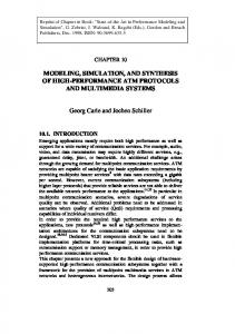
A fuzzy set is called fuzzy number e a if it is normal and convex and if there is only one element x ¯ ∈ R with the degree of membership µea (¯ x) = 1. In addition, the membership function µea (x), x ∈ R, has to be at least piecewise continuous. Certain types of fuzzy numbers, either symmetric or unsymmetric, are commonly used, such as the triangular fuzzy number (Figure 1a) and the Gaussian fuzzy number (Figure 1b). They are defined by their membership functions µea (x) and their left-hand and right-hand worst-case deviations αl and αr , or their left-hand and right-hand standard deviations σl and σr respectively. The extension principle [5] can be adapted to fuzzy numbers, thus enabling the evaluation of mathematical operations like addition, multiplication etc.
3
The Transformation Method
The Transformation Method was introduced by Hanss in its reduced, general, and extended form [1, 2], the later being a combination of the two aforementioned. The method allows dealing with fuzzy numbers in a very comfortable and structurized manner. The following is a rather short introduction to the transformation method, details can be found in the literature mentioned above. Let us assume a system with n uncertain parameters pei , i = 1, 2, . . . , n, characterized by fuzzy numbers and show the steps taken when using the reduced transformation method.
In the first step, similar to conventional fuzzy arithmetic, each fuzzy number is discretized (Figure 2). The interval [0,1] of the membership function µea is divided into m intervals of length ∆µ = 1/m at (m + 1) equally spaced membership levels µj , j = 0, 1, . . . (m + 1). An interval [a(j) , b(j) ] belonging to each level j can be identified that way, leading to a decomposed representation of each fuzzy number. The next step is the transformation of the input intervals. Effective on each level j separately, boundary values of the (j) (j) intervals ai and bi of each fuzzy parameter pei , i = 1, 2, . . . , n, are combined in every possible way. In this manner, b (j) on each membership level j are generated. Each of these samples of possible all possible input combinations X i parameter values is an input set to the problem to be evaluated. b (j) yields an equal amount of computed results Z b(j) on The evaluation of the problem carried out for each sample X i (j) b each level j. To gain the fuzzy output qe of the evaluation the results Z have to be retransformed and recomposed.
The retransformation itself contains two steps. First, going down through the (m + 1) levels from µ = 1 to µ = 0, one determines the minimum and maximum values of the results belonging to each level, Z (j) = [a(j) , b(j) ]. In the second part a result in the form of a fuzzy number is ensured by the recursive formulas � � � � and b(j) = max b(j+1) , b(j) with j = 0, 1, . . . , m − 1. (2) a(j) = min a(j+1) , a(j) k
k
For the level j = m, we find a(m) = min k (j)
k (m)
zˆ
�
= max k
k (m)
zˆ
�
= b(m) , where k zˆ(m) is the kth sample in
this level. By recomposing the intervals Z according to their levels of membership µj , the fuzzy output qe of the fuzzy-parameterized system can be obtained. Furthermore, it is possible to analyze the influence of each fuzzy input parameter pei on the overall fuzzy result qe. (j) For these purposes, Hanss [2] introduced the gain factors ηi , that express the effect of the uncertainty of the ith parameter pei on the uncertainty of the output qe of the problem at the membership level µj . To obtain a non-dimensional form of the influence measures with respect to the usually different physical dimensions of pei , the standardized mean gain factors κi can be determined as an overall measure of influence. As a relative measure of influence, their normalized values ρi can be determined as degrees of influence for i = 1, 2, . . . , n. The reliability of these influence measures has been proven in [3]. If the fuzzy-parameterized model is expected to show non-monotonic behavior with respect to a number of fuzzy-valued parameters the general transformation method is recommended. It takes into account additional values associated to the uncertain parameters, specifically values lying in between the interval boundary values [a(j) , b(j) ]. The transformation method includes these values in the transformation of the fuzzy input parameters and the retransformation of the results. The general transformation method naturally requires a higher computational effort for the same discretization number as the reduced method, as there are much more parameter variations and thus a higher number of problem evaluations. The extended transformation method is a combination of the reduced and the general form. Input parameters that show a non-monotonic behavior can be treated according to the general method, the remaining according to the reduced method, incorporating thus the benefits of both methods. A drawback of the transformation method may be seen in the possibly sizable number of system evaluations that is required, in particular if the general form of the transformation method is considered together with a significant number of fuzzy-valued model parameters. This may lead to high computational costs, especially if large-scale models are intended to be simulated. Thus, multiple occurrence of parameter combinations should be avoided. Further reductions of the computational costs can be achieved by the use of the extended transformation method or a special approach based on piecewise multilinear sparse-grid interpolation [4].
4
Examples
In the following, two examples on the practical application of the transformation method are shown. The uncertain b (j) are computed in a preprocessing step. The parameters pei of the problem are transformed and all parameter sets X i problem is then evaluated for each parameter set by a commercial finite element code. The postprocessing step includes the retransformation and the recomposition of the result as well as its interpretation. The examples will simulate and analyze the vibration behavior of automotive components: first, a circuit board, and second, an engine hood.
Fz
z
y x
uz Figure 3: Plate with fixed support on two sides.
4.1
Circuit Board
The circuit board is part of an automotive control unit. This unit is fixed in a slot in the engine compartment of a car with a thin rubber layer between the unit and the slot. In an approximation, we regard the circuit board of the unit fixed on two sides, modeling the support conditions of the unit (Figure 3). The board itself is approximated by a square plate with a side length of a = 0.2 m and a thickness of t = 1 · 10−3 m. The material shall be characterized by the Young’s modulus E, the mass density ρ, and Poisson’s ratio ν. The system is undamped. For the computations with uncertain material parameters, the thickness t, the density ρ, and Young’s modulus E will be represented by triangular fuzzy numbers tfn(¯ p, αl , αr ), each varying in a range of ±5%, pe1 = e t = tfn(t, 5% t, 5% t) ,
t = 1 mm = 1 · 10−3 m ,
(3)
ρ = 7800 kg m
(4)
e = tfn(E, 5% E, 5% E) , pe3 = E
E = 2.1 · 1011 N m−2 .
pe2 = ρe = tfn(ρ, 5% ρ, 5% ρ) ,
−3
,
(5)
A second series of computations is carried out with uncertain support parameters, in order to simulate the effects of the fixation in the slot. The intention is to investigate the transition from a fixed support to a clamped support. Here, the term fixed support refers to a support with fixed degrees of freedom with regard to the displacement in xand y-directions as well as an inhibited rotation with respect to the z-axis as these movements are inhibited by the fixation in the slot. If the board is regarded as clamped on both sides, the degrees of freedom not covered by the fixed support, i.e. the displacement in z-direction u(z) and the rotations rot(y) and rot(x) with regards to the y- and x-axis, respectively, are set to zero additionally. To simulate the transition between these two stages, we introduce linear springs (or torsional springs in case of the rotational degree of freedom) for the three degrees of freedom not covered by the fixed support. This applies to all nodes on the regarded sides of the board and enables us to reproduce a quasi-clamped state by varying the stiffness of these springs. The clamped state is sufficiently reproduced if the first 25 eigenfrequencies of the clamped and quasi-clamped model are identical with respect to the first decimal place. We find the following values for the spring stiffnesses for the quasi-clamped stage, ku(z),clamped krot(y),clamped krot(x),clamped
= = =
1 · 107.5 N m−1 ,
(6)
1 · 10
4.5
Nm
,
(7)
1 · 10
2.5
Nm
.
(8)
−1 −1
As some of these stiffnesses of the springs are quite high, it will not be sufficient to represent them by fuzzy numbers in between the fixed support with a chosen kfixed = 1 Nm−1 and the given values for the quasi-clamped state. Unless one is willing to work with a very high discretization number m and to accept an extremely high number of computations, it is advisable to identify the exponent of the spring stiffnesses as the uncertain parameter. This assumption leads to the following triangular fuzzy input parameters: the exponents of the stiffness of the linear spring ku(z) and the
1.0 0.9 0.8
1.0
fe1
fe2
fe4
fe3
fe5
fe6
fe7
0.9 0.8 0.7
0.6
0.6
µfer (f )
0.5
fe4
fe3
fe5 fe6 fe7
0.5
0.4
0.4
0.3
0.3
0.2
0.2
0.1
0.1
0 0
fe2
µfer (f )
0.7
fe1
100
200
300
400
500
600
f /Hz Figure 4: Membership functions µfer (f ) of the eigenfrequencies fer , r = 1, 2, . . . , 7, of the circuit board with uncertain material parameters.
0 0
100
200
300
400
500
600
f /Hz Figure 5: Membership functions µfer (f ) of the eigenfrequencies fer , r = 1, 2, . . . , 7, of the circuit board with uncertain support parameters.
stiffness of the torsional springs krot(y) and krot(x) , p1 ), 0) , pe1 = e ku(z) = tfn(k u(z) , αl (e
pe2 = e krot(y) = tfn(k rot(y) , αl (e p2 ), 0) ,
pe3 = e krot(x) = tfn(k rot(x) , αl (e p3 ), 0) ,
k u(z) = 7.5 , αl (e p1 ) = 6.5 ,
(9)
k rot(y) = 4.5 , αl (e p2 ) = 3.5 ,
(10)
krot(x) = 2.5 , αl (e p3 ) = 1.5 .
(11)
As can be seen, the right deviation αr of each of the three uncertain parameters is zero, as the mean value stands for the clamped state and we are not interested in any further variation of the spring stiffnesses. For the simulation of the uncertain system, a combination of commercial programs is used. The pre- and postprocessing steps are performed in MATLAB, the finite element computations by the software package ANSYS, and the communication between these components is accomplished by the optimization software OPTISLANG. The board is discretized by a simple mesh using four node shell elements. The effects of the above noted fuzzy parameterized uncertainties on the values of the eigenfrequencies of the system are investigated for both material and support uncertainties. Figure 4 shows the membership functions µfer (f ), r = 1, 2, . . . , 7, of the eigenfrequencies of the circuit board with uncertain material parameters in the frequency range from 0 to 600 Hz. For this simulation, the reduced transformation method with a discretization number of m = 10 is used. The triangular shape of the input parameters is directly reflected by the result, showing the linearity of the problem. Even though an increasing deviation from the crisp value at µfer (f ) = 1 can be noted with increasing frequency f , the relative deviation remains at the same value for each of the eigenfrequencies. Figure 5 shows the equivalent computation done with uncertain support parameters. The reduced transformation method with a discretization number of m = 20 is applied. The first three eigenfrequencies clearly show the transition from an almost rigid body motion (note that the lowest value for the spring stiffnesses is not zero) to the value of the crisp eigenfrequency. The abrupt decrease of the values at each crisp eigenfrequency is due to the shape of the fuzzy-parameterized input as described above. The solid lines refer to exactly the same seven eigenfrequencies as in Figure 4. The dashed lines intruding the figure from the right belong to eigenfrequencies whose crisp values lie above f = 600 Hz. For example, at a frequency of f = 500 Hz, there is a clear influence from r = 7 different eigenfrequencies. In accordance with the results shown in Figure 4, the analysis of the system as mentioned in Section 3 shows that the degrees of influence of the uncertain material parameters pei , i = 1, 2, 3, i.e. thickness, mass density and Young’s modulus, are at the constant value ρi (fer ) = 0.333 for each of the overall computed r = 25 eigenfrequencies. This confirms the results discussed above. Figure 6 shows the degrees of influence ρi (fer ) associated to each eigenfrequency and separately for each of the i = 3 uncertain parameters pei for the system with uncertain support parameters. We remember that pe1 affects the stiffness
0.31
ρ1 (fer ) 0.305
5
10
15
20
25
5
10
15
20
25
5
10
15
20
25
0.22
0.21
ρ2 (fer ) 0.2
0.5
0.49
ρ3 (fer )
0.48
0.47
Number of Eigenfrequency fer
Figure 6: Degrees of influence ρi (fer ), r = 1, 2, . . . , 25, of the eigenfrequencies of the circuit board with uncertain support parameters. of the linear spring in z-direction, pe2 and pe3 affect the stiffness of the torsional spring, respectively. Even though the variations of ρi (fer ) may be relatively small, distinct similarities in the characteristics of ρ1 (fer ) and ρ2 (fer ) can be found. This pattern is almost exactly mirrored by the normalized standard mean gain factor of the third uncertain input parameter. Local maxima and minima in the characteristics are clarified by dotted lines and underline these observations. As a result, we can state that the stiffnesses of the linear spring ku(z) and the torsional spring krot(y) have a similar influence on the system; the stiffness of the third uncertain parameter, the torsional spring krot(x) , exhibits opposite character. We can find an explanation of this behavior based on the shapes of the eigenmodes.
4.2
Engine Hood
Addressing a finite element problem of higher complexity, the transformation method is applied to simulate and analyze the vibration behavior of an engine hood with uncertain model parameters. Specifically, we consider the engine hood of the roadster Mercedes SLK, which is shown in its top and bottom view in Figure 7. The engine hood consists of an upper sheet metal of thickness t1 =0.8 mm and a bottom metal frame of thickness t2 =0.7 mm displayed in different shades of grey. Both components consist of the same material. The thicknesses of the metal sheets as well as the mass density ρ = 8400 kg m−3 of the material will be identified as uncertain parameters in the following. They are quantified by symmetric quasi-Gaussian fuzzy numbers with a standard deviation of 3% which corresponds to a worst-case deviation of ±9% from the center values. The Young’s modulus E = 2 · 1011 N m−2 and Poisson’s ratio ν = 0.314 will be treated as crisp parameters. For the simulation of the uncertain system, the in-house program FAMOUS uses the transformation method in conjunction with the commercial finite element software package MSC.Marc. The engine hood is discretized according to the mesh in Figure 7, consisting of 1 889 nodes and 2 235 thin-shell elements – most of them four-node elements, some of three-node type. As the output values of the system, the first six uncertain eigenfrequencies fer of the engine hood are determined. The system is undamped. To simulate the support conditions of the engine hood on the car body, the degrees of freedom of the nodes at locations A, B1 , and B2 in Figure 7 are set to zero.
a
B1
b
A
B2 Figure 7: Mercedes SLK engine hood including the finite element mesh and the locations A, B1 , and B2 of the support: (a) top view; (b) bottom view (courtesy of DaimlerChrysler AG, Stuttgart). The uncertain parameters are transformed using a discretization number of m = 10. Monotonic behavior of the fuzzy input parameters is to be expected. Therefore, the reduced transformation method is applied. Figure 8 shows the membership functions µfer (f ) of the computed eigenfrequencies fer , r = 1, 2, . . . , 6. It can easily be seen that the absolute uncertainty of the eigenfrequencies increases with the growing value of the respective eigenfrequency. Nonetheless, the relative deviation of the values is at about ±9% which matches with the assumed maximum deviation of fuzzy input parameters. Therefore, the increasing uncertainty is due to increasing values of the computed eigenfrequencies. Two of the eigenmodes corresponding to the second and the sixth eigenfrequency are shown in Figure 9 and Figure 10 to visualize the type of oscillations. In these diagrams, the amplitudes of the displacements are quantified by a gray scale, where darker gray tones symbolize higher amplitudes. From an analysis of the computations, the standard mean gain factors κi (fer ) and their normalized values ρi (fer ) can be determined. These are measures of the influence of the uncertain parameter pei , i = 1, 2, 3, on the rth eigenfrequency fer , r = 1, 2, . . . , 6. Figure 11a and Figure 11b show the influence measures for each of the six eigenfrequencies. The black block refers to the input parameter pe1 , the thickness of the upper sheet metal, the dark grey block to the input parameter pe2 , the thickness of the bottom frame, and the light grey block to pe3 , the mass density. Focusing on the influence of the uncertain parameters pe1 and pe2 , we can see that the influence of pe2 is significantly higher than the influence of pe1 if the engine hood oscillates in its second eigenmode. However, if the sixth eigenmode is considered, we notice the opposite situation. As an explanation of this phenomenon, we examine the shape of the respective eigenmode from Figures 9 and 10. The second eigenmode in Figure 9 represents the first bending mode of the hood about an in-plane axis that is orthogonal to the axis of symmetry of the hood. In this eigenmode, the stiffness-inducing bottom frame of the hood, which is characterized by the uncertain thickness parameter pe2 , will definitely be the determining factor of the oscillation, 1.0
fe1
µfer (f )
fe2
fe4
fe3
fe5 fe6
0.5
0.0
0
20
40
f /Hz
60
80
100
Figure 8: Membership functions µfer (f ) of the first six uncertain eigenfrequencies fer , r = 1, 2, . . . , 6, of the engine hood.
f 2 = 20.37 Hz Figure 9: Eigenmode of the engine hood for the second eigenfrequency with its modal value f 2 = 20.37 Hz.
f 6 = 92.62 Hz Figure 10: Eigenmode of the engine hood for the sixth eigenfrequency with its modal value f 6 = 92.62 Hz.
a
b
100
κi (fer ) Hz
κ1 κ2
50
1.0
ρi (fer )
ρ1
0.5
ρ3
ρ2
κ3
0
fe1 fe2 fe3 fe4 fe5 fe6
0.0
fe1 fe2 fe3 fe4 fe5 fe6
Figure 11: (a) Standardized mean gain factors κi (fer ) and (b) normalized degrees of influence ρi (fer ) with light gray for i = 1, dark gray for i = 2, and black for i = 3.
exhibiting a predominant influence on the uncertainty of the eigenfrequency fe2 . Alternatively, the sixth eigenmode in Figure 10 represents a localized form of vibration, which primarily affects the upper sheet of the hood in the area located inside the bottom frame. For this reason, the uncertainty of the eigenfrequency fe6 is considerably more influenced by the uncertain thickness parameter pe1 of the upper sheet, than by the respective property e t2 of the bottom frame.
5
Conclusions
A fuzzy arithmetical approach for the simulation and analysis of systems with uncertain parameters has been presented. In this concept, the uncertain parameters are modeled by fuzzy numbers, and the fuzzy-parameterized models are evaluated by the use of the transformation method in conjunction with existing simulation environments, such as commercial finite element software. Both examples presented support these claims. In addition, both examples are a good foundation for further research such as the frequency response of the systems, especially with respect to uncertain support parameters. An application of the described methods on even more complex real-world problems is also intended.
6
Acknowledgments
The financial support by the Robert Bosch GmbH, Stuttgart, Germany, is gratefully acknowledged.
References [1] M. Hanss. The transfomation method for the simulation and analysis of systems with uncertain parameters. Fuzzy Sets and Systems, 130:277–289, 2002. [2] M. Hanss. The extended transformation method for the simulation and analysis of fuzzy-parameterized models. International Journal of Uncertainty, Fuzziness and Knowledge-Based Systems, 11(6):711–727, 2003. [3] M. Hanss and A. Klimke. On the reliability of the influence measure in the transformation method of fuzzy arithmetic. Fuzzy Sets and Systems, 143:371–390, 2004. [4] A. Klimke and B. Wohlmuth. Computing expensive multivariate functions of fuzzy numbers using sparse grids. Technical report, Institute of Applied Analysis and Numerical Simulation, University of Stuttgart, 2004. [5] L. A. Zadeh. Fuzzy sets. Information and Control, 8:338–353, 1965.