Modeling and Visualization of 3D Polygonal Mesh Surfaces using Geometric Algebra M. D. Zaharia ∗ , L. Dorst Informatics Institute, Faculty of Sciences, University of Amsterdam, Kruislaan 403, 1098 SJ, Amsterdam, The Netherlands
Abstract The language of geometric algebra can be used in the development of computer graphics applications. This paper proposes a method to describe a 3D polygonal mesh model using a representation technique based on geometric algebra and the conformal model of the 3D Euclidean space. It describes also the stages necessary to develop an application that uses this formalism. The current application was used to validate the implementation of the main abstract operations characteristic to a geometric algebra computational environment (programming module GAP). The data structures that characterize this geometric algebra based modeling approach as well as the implementation of geometric algebra based methods for model visualization/transformation are developed in detail. The paper emphasizes the elegance and generality of the geometric algebra approach referring also to the necessary computational resources. Key words: geometric algebra, conformal model, polygonal mesh, visualization, graphics data structures and data types, boundary representations, surface representations, geometric transformations
∗ Corresponding author. Tel : +31 (20)-525.75.17, Fax : +31 (20)-525.76.90, Email address:
[email protected] (M. D. Zaharia). URL: http://carol.science.uva.nl/∼marius (M. D. Zaharia).
Preprint submitted to Computers & Graphics
15 September 2003
1
Introduction
Through its rules, geometric algebra can be considered as a formal language suitable to specify the behavior of various natural systems and capable of providing a unified framework to solve geometrical problems in wide areas of applicability. Based on the 19-th century works of Grassman and Clifford, geometric algebra associates a geometric semantics to the ”pure algebraic” products specific to a Clifford algebra (see [4,7]). Geometric Algebra introduces algebraic operators directly interpretable as the geometric operations of spanning, rotation and projection of subspaces. The main products manipulating the algebraic entities (like blades or multivectors) are: the inner product (denoted •), the outer product (denoted ∧), the geometric product (usually denoted by the simple juxtaposition of its operands). These products and a lot of related operators (meet, join, contraction, delta product) allow the description of the intrinsic spatial relations characteristic to geometric applications in a concise, coordinate-free way. Techniques based on the application of algebraic manipulation rules find their applicability in various science fields as physics, computer science, robotics, signal processing or astronomy(see [1] or [12]). The scientist that (after almost one hundred years since Clifford passed away) emphasized the huge possibilities offered by Geometric Algebra, as a universal language for geometric calculus is David Hestenes ([5]). This paper does not propose itself to give the description of the computational rules characteristic to geometric algebra; the interested reader can find these in [4]. However, some detailed algebraic manipulation is presented so that the reader may form an opinion about the kind of work necessary to derive a geometric algebra based model that fulfills the requirements of a specific application. The fundamental products characteristic to a geometric algebra environment are: • the outer product a grade increasing, linear operator geometrically related to the spanning concept (for example the outer product of two vectors a, b produces a bivector that characterizes the plane spanned by a when its origin sweeps b) • the inner product a grade decreasing, linear operator that is geometrically related to orthogonality and metric concepts • the geometric product that, in case of vector operands, is defined by: ab = a • b + a ∧ b. It is multilinear and produces usually mixed grade results. For example, if its operands Ar and Bs are homogeneous multivectors of grade r and s their geometric product Ar Bs will usually contain homogeneous components of grades: |r-s|, |r-s+2|, . . ., r+s. The elementary operands of the geometric algebra Gn are the subspaces (called also blades). A blade is a homogeneous entity, characterized by its grade (an 2
integer related to the subspace dimension), and can always be factorized as an outer-product of vectors: Bk = v1 ∧ v2 ∧ . . . ∧ vk
n The blades of grade k form a -dimensional subspace of the multivectors k space. Another geometric algebra entity that is suitable for computer graphics applications is the versor . It can be written as a geometric product of vectors: V = v1 v2 . . . vk A blade is a special type of versor, since in case of orthogonal factors the outer product of vectors (characteristic to the blade definition) corresponds to a geometric product of vectors (characteristic of a versor definition). In geometric algebra any orthogonal transformation (including reflection) is accomplished by geometric multiplication through: T (x) = VxV−1
(1)
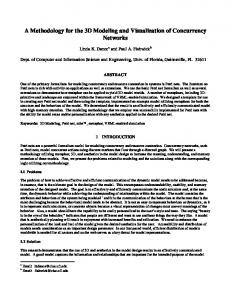
If V is a vector (1-grade blade) the formula corresponds to a reflection, if it is a geometric product of two vectors v1 and v2 the transformation is a rotation (see [6]). In this last case, the bivector v1 ∧ v2 specifies the rotation plane (its dual represents the rotation axis) and the angle between v1 and v2 corresponds to twice of the rotation angle. Note that the same routine can be used to reflect a vector or to rotate a vertex (or even a plane bivector). Figure 1 shows three instances of a wineglass. The second is obtained through a rotation and the third through a reflection relative to a plane. All the transformations were computed using the function ApplyOrthoTransform() (see section 3.2). The most general computational elements, manipulated by the algebraic operators are the multivectors. They are non-homogeneous (i.e. mixed grade) entities that, in case of the algebra built over a 3D Euclidean space, are obtained by summing scalars, vectors, bivectors (2-blades) and trivectors. The set of multivectors generated by adding and/or multiplying vectors from the 3D Euclidean space forms (together with the multivector sum, the geometric product and the scalar-multivector multiplication) the geometric algebra of the 3D Euclidean space. In general a Clifford algebra is the algebra (M, +, ◦) where M is a set of multivectors, + is the multivector addition (having the usual meaning when both operands are scalars, vectors, bivectors etc.), ◦ is the geometric product. 3
The multivectors are built as sums of geometric products of vectors from a n-dimensional vector space, denoted V n . The Clifford algebra is sometimes denoted C`n (V n ) in order to explicitly mention the vector space over which the algebra was built. Usually V n = Rn but other cases may also be possible as mentioned below. If the vector space is pseudo-Euclidean, one notation frequently used is C`p,q where p, q denote the number of V n basis vectors with positive, and respectively negative signature (n = p+q). Similarly, the notation C`p,q,r additionaly specifies the number of null basis vectors (r). If r 6=0, the corresponding algebra is called degenerate. The multivector set constitutes a 2n -dimensional vector space. The main difference between Clifford algebra (C`n ) and geometric algebra (denoted Gn ) is that the latter emphasizes the geometric semantics of the algebraic entities. Considering known all the basic algebraic manipulation rules, the present paper continues with a short presentation of the conformal model of the 3D Euclidean space and uses the powerful representational capabilities of this model to provide the application programmer with the methods necessary to extract the information needed for the visualization of a polygonal mesh.
2
The conformal model
The conformal model represents the points of the Euclidean space E n using the geometric algebra of a higher dimensional space Rn+1,1 (called also the conformal space). The role of the two extra dimensions is elegantly and intuitively presented in [11] which emphasizes the relation between this model and the concept of stereographic projection. Some authors call the conformal geometric algebra the algebra of spheres, emphasizing that in this algebra the blades represent spheres . In the conformal model, a Euclidean point (labeled by the Euclidean vector ~x) is represented by conformal vector x. Obviously, not all the conformal vectors represent Euclidean points. The inner product of two conformal vectors is closely related to the Euclidean distance between the points they represent: 1 1 x • y = − (~x − ~y )2 = − (x − y)2 2 2
(2)
This implies x2 = x • x = 0 i.e. the Euclidean points are represented by null vectors. All these null vectors make up the null cone of the conformal space. Two null vectors have special significance: e∞ denotes the ”point at infinity” and e0 corresponds to the Euclidean origin. These vectors can be regarded as forming a null basis of the Minkowski subspace R1,1 of Rn+1,1 . 4
One possible way to build a correspondence between Euclidean points and conformal vectors is a technique called projective split ([8,10]). This method consists of establishing a linear mapping between the vectors of a higher dimensional space V m and a subset of the multivectors of a lower dimensional geometric algebra Gn (m > n). In the concrete case of the conformal split: m = n + 2, the original higher dimensional space is a Minkowski space (V m =Rn+1,1 =Rn ⊕ R1,1 ) and the split is done relatively to a bivector (the one formed through the outer-multiplication of the null basis vectors of R1,1 ). In this model, a vector from the Euclidean space Rn is regarded as the rejection, relative to the null plane (with tangent bivector E=e0 ∧e∞ ) of the corresponding vector from the Minkowski space Rn+1,1 . Denoting the conformal vectors with bold face lower case letters and the Euclidean vectors with attached arrows, the relations expressing the mapping between the points from Euclidean space and vectors of conformal space can be shown to be: 1 2 x = ~x + e0 + x ~ e∞ 2
(3)
and inversely ~x = (x ∧ E)E
(4)
In the conformal model, all affine entities (e.g. lines or planes) of the 3D Euclidean space as well as the Euclidean spheres or circles are represented as 5D subspaces (blades). This confers a huge computational advantage when these entities are manipulated through geometric algebra operators. From the transformational point of view, there is a correspondence between the conformal transformations in the Euclidean space and the orthogonal transformations (in fact even isometries) of the null conformal cone. Any isometry in the null cone (in conformal space) defines a conformal transformation in the corresponding Euclidean space. Inversely, any conformal transformation in the Euclidean space induces two isometries (that differ only by a sign) in the conformal space (see [11]). Consequently all the (Euclidean) conformal transformations are simply achieved by a ”versor like” geometric multiplication in conformal space (see (1)). This motivated in fact the name of this model. Complex operations like intersection and union are accomplished in a simple, uniform way using subspace operations (meet and join). Some detailed algebraic manipulations that allow extracting useful information from the blade-representation of different geometric entities are given below (see also [10]). Other examples of detailed algebraic manipulation may be seen in [13]. 5
3
Development of a computer graphics application using geometric algebra
When developing a computer graphics application, the designer has to identify first the geometric algebra entities (blades, versors, multivectors) that are best suited to model the specific application objects (see section 3.1). He has to remember that one single entity could encode a variety of information and has equally to consider the most efficient ways to extract this information. The abstract operations specific to geometric algebra (for example the geometric product) are expensive to use and minimizing their number must be an implementation goal. After building the model storage structure, the programmer must design the associated access methods as well as those necessary to transform or to visualize the model (see 3.2). Sometimes the programming environment used for the application development requires a specific format for the information to be visualized. This could imply the use of format conversions between the geometric algebra based model and the particular data visualization format. The current application example allows the visualization of a polygonal mesh model that can be arbitrarily rotated or reflected. The shading is accomplished using the Phong illumination model.
3.1
Choosing the geometric algebra entities that make up the model
As it was already mentioned, Euclidean points are represented by null conformal vectors. Papers like [10] and [9] detail the conformal representations for Euclidean lines, circles, spheres and their algebraic properties. For example a line passing through the (Euclidean) points P, Q is represented by the conformal blade e∞ ∧ p ∧ q and the sphere passing through 4 Euclidean points (denoted P, Q, R, S) is represented by the conformal blade p∧q∧r∧s. Here we will accord special attention to the conformal blades representing Euclidean planes because they are used in our polygonal mesh model. A plane that passes through the (Euclidean) points P, Q, R labeled by the Euclidean vectors p~, ~q, ~r respectively has the conformal representation ∆=e∞ ∧ p ∧ q ∧ r; this simple outer-product (4-vector) codifies a lot of information necessary for the graphic visualization of the plane surface (normal, directance - i.e. the oriented distance to the origin) and quantitative information related to the triangle PQR, for example its area. ∆ does not encode the triangle spatial location, it specifies only an ”area element”. The following derivations are examples of how general geometric algebra manipulation rules determine the geometric semantics associated to algebraic entities. Developing the outer 6
product results in: ∆ = e∞ ∧ p ∧ q ∧ r 1 1 1 = e∞ ∧ (~p + e0 + p~ 2 e∞ ) ∧ (~q + e0 + ~q 2 e∞ ) ∧ (~r + e0 + ~r 2 e∞ ) 2 2 2 1 2 1 2 = (e∞ ∧ p~ − E) ∧ (~q + e0 + ~q e∞ ) ∧ (~r + e0 + ~r e∞ ) 2 2 1 2 = (e∞ ∧ p~ ∧ ~q + E ∧ p~ − E ∧ ~q) ∧ (~r + e0 + ~r e∞ ) 2 = e∞ ∧ p~ ∧ ~q ∧ ~r − E ∧ p~ ∧ ~q + E ∧ p~ ∧ ~r − E ∧ ~q ∧ ~r = e∞ ∧ p~ ∧ ~q ∧ ~r − E ∧ (~p ∧ ~q + ~q ∧ ~r + ~r ∧ p~) = e∞ ∧ p~ ∧ ~q ∧ ~r − E ∧ (~q − p~) ∧ (~r − p~) = e∞ (~p ∧ ~q ∧ ~r) − e∞ • (~p ∧ ~q ∧ ~r) − (E(~q − p~)) ∧ (~r − p~) +(E • (~q − p~)) ∧ (~r − p~) = e∞ (~p ∧ ~q ∧ ~r) − (E(~q − p~)) ∧ (~r − p~) (5) The plane (PQR) (represented by a Euclidean bivector that gives the plane direction and orientation) can then be recovered from: e∞ ∆ = e∞ • ∆ = e∞ 2 (~p ∧ ~q ∧ ~r) − e∞ (E(~q − p~)) ∧ (~r − p~) = e∞ ∧ (~q − p~) ∧ (~r − p~) = (~q − p~) ∧ (~r − p~) ∧ e∞ = (~q − p~) ∧ ((~r − p~)e∞ ) ⇒
E • ∆ = e0 • (e∞ • ∆) = e0 • (e∞ ∧ (~q − p~) ∧ (~r − p~)) = −(~q − p~) ∧ (~r − p~)
(6)
where (~q − p~) ∧ (~r − p~) represents exactly the tangent bivector of the plane that passes through the Euclidean points P, Q, R. Simple computational expressions for the plane directance (distance to the origin) and normal are obtained noticing that the plane that passes through P, Q, R can be dually represented by the conformal vector (∆∗ ). Here, the superscript signifies the dual in conformal space i.e. the blade of the orthogonal complement, which is computed through division by the volume element of the conformal space. If we denote by ~n the plane normal and by δ its directance then: ∆∗ = (e∞ ∧ p ∧ q ∧ r)∗ = µ(~n + δe∞ )
(7)
where ~n is a unit Euclidean vector. Indeed, the blade ∆∗ is a vector, it is the dual of a 4-grade blade in a 5-dimensional space. The complete proof of (7) is 7
given in [10]. The scalar factor µ (µ2 = (∆∗ )2 = ∆2 ) is, as will soon be proven, related to the area of the triangle PQR. Further, the values of normal and directance can be obtained from ∆: δ = p~ • ~n = ~q • ~n = ~r • ~n = −
e0 • ∆∗ µ
(8)
1 ∗ 1 (∆ ∧ E) • E = E • (∆∗ ∧ E) = E • (~n ∧ E) = (e0 ∧ e∞ ) • (E ∧ ~n) µ µ = (e0 • (e∞ • (e0 ∧ e∞ ∧ ~n))) = −e0 • (e∞ ∧ ~n) = ~n (9) Denoting by a, b, c the lengths of the three sides of the triangle PQR (i.e. a=| p~ − ~q |, b=| ~q − ~r |, c=| ~r − p~ |) and by A the area of the triangle, we may 2 verify that: A = − ∆4 and consequently µ = 4A2 . Indeed, taking into account (2): ∆2 = (e∞ ∧ p ∧ q ∧ r) • (e∞ ∧ p ∧ q ∧ r) e∞ • e∞ e∞ • p e∞ • q e∞ • r p • e∞ e ∞ • e ∞ q • e∞ r • e ∞ = q•e q • p q • q q • r ∞ r • e∞ r•p r•q r•r 0 −1 −1 −1 −1 p • q p • r −1 e∞ • e∞ q • e∞ r • e∞ = −1 0 q • r − = −1 q • p q • q q • r −1 r • q 0 −1 r • p r•q r•r −1 0 p • r −1 0 p • q −1 q • p q • r + −1 q • p 0 −1 r • p 0 −1 r • p r • q
= (r • q)2 + (q • p)2 + (r • p)2 − 2(r • q)(p • r) −2(p • q)(q • r) − 2(p • q)(r • p) 1 1 1 1 1 1 1 = b4 + a4 + c4 − a2 b2 − b2 c2 − c2 a2 = (b2 − a2 − c2 )2 − a2 c2 4 4 4 2 2 2 4 1 = (2ac cos(B))2 − a2 c2 = a2 c2 (cos2 (B) − 1) = −a2 c2 sin2 (B) 4 8
= −(2area)2 = −4A2 The derivations above show how specific geometric information can be recovered from the algebraic representation. This type of computations emphasize that a proper geometric algebra based model of the polygonal mesh can store the conformal blades that represent the face planes. These blades can be easily transformed using (1) and allow also the recovery of face normals, necessary for color computations. However, the precise spatial location of the polygonal faces cannot be recovered; formula (8) gives only their distances to the origin. One way to specify the positional information would be to explicitly store the vertices locations; this method was preferred in our implementation. The positions of the vertices might also have been recovered from the blades specifying the face-plane information and the array describing the face-vertex relation, using the meet operator. The same technique may be used to recover the edges of the polygonal mesh. For the present visualization application the explicit representation/manipulation of the edges is not necessary.
3.2
Representing polygonal data using geometric algebra
The geometric algebra specific operands (SPACE, BLADE, HOMOGENEOUS MULTIVECTOR, MULTIVECTOR, VERSOR) and operators (geometric product, outer product, inner product, meet, join) were implemented in a specialized package, GAP. The implementation is based on linked lists representations, the package is documented ([14]) and freely available. Its description will not be further detailed here. The polygonal mesh visualization application was used to verify the validity of GAP implementation and to evaluate its performance when used in a computational intensive application. Details concerning the usage of the geometric algebra primitives in computations characteristic to the visualization process are given below. The data type used to specify the polygonal mesh is: typedef struct pmga{ int nvert, nfaces; // number of vertices, number of faces BLADE *vertices; // array of 1-grade (conformal) blades; // every element specifies a vertex BLADE *plpolig; // array of 4-grade (conformal) blades; every // array element represents a face plane int **faces; // array specifying the face-vertex relation COLOR *cul; // array of vertex colors } *PMESH_GA; The visualization of a given polygonal mesh that rotates by a specific angle was done in OpenGL. The application program computes the vertices col9
ors using the Phong local illumination model. The computations necessary to visualize this model were accomplished using geometric algebra operators acting on conformal entities, represented using the null conformal basis. The interpolative shading was left to the OpenGL rendering engine. One can easily notice that the vertex normals are not part of the model storage structure, since normals do not transform simply under general linear transformations. However, the vertex color computation requires to determine these normals. The extraction of this information from the model data is accomplished during the visualization stage of the application. The model transformation (rotation or reflection) is applied to the surface elements ”plpolig” and of course to the vertices. As an example, the function performing the vertex color computation is specified below: COLOR ColorComputation_GA(PMESH_GA p, int nv) // computes the color of the vertex nv of the polygonal mesh // the Phong local illumination model is applied { BLADE normvert, t, r, LR1; //vertex normal COLOR crez; int i, j, n; double c1, c2, a, b, c, m; //the vertex-face relation (arrays vfrel[][] and fadv[]) //is built once in the initial stage of the application for(i=0, a=b=c=0.0; iplpolig[vfrel[nv][i]], Jpsc): //Jpsc = original pseudoscalar Dual1(p->plpolig[vfrel[nv][i]], Jpscm); //Jpscm = reflected pseudoscalar t=VectorConformalToEuclidean(t1); m=SquaredMagnitude(t); if(m>0) { m=sqrt(m); a+=Extract_X(t)/m; b+=Extract_Y(t)/m; c+=Extract_Z(t)/m; } FreeHMV(t1); } normvert=(flagm==0)?VectorEuclidean(csp, a, b, c): normvert=VectorEuclidean(csp, -a, -b, -c); //reflection reverses normals c1=cosangle(LEuc, normvert); //LEuc specifies the light source direction r=ApplyOrthoTransform(normvert, L); //compute L reflected with respect to normvert LR1=VectorConformalToEuclidean(r); FreeBlade(r); c2=cosangle(LR1, VEuc); FreeBlade(LR1); crez.R=camb.R+cdif.R*c1+cspec.R*pow(c2, cPhong); 10
crez.G=camb.G+cdif.G*c1+cspec.G*pow(c2, cPhong); crez.B=camb.B+cdif.B*c1+cspec.B*pow(c2, cPhong); return crez; } Every face normal is computed using formula (9). Let M be an arbitrary vertex of the polygonal mesh. The vertex normal is obtained by averaging the normals of the faces adjacent to M. The Phong local illumination model requires the determination of the vector r that is the reflection of the light source vector relatively to the vertex normal. This is done using the same function that rotates the face-planes (their conformal blades representations) and the mesh vertices. The function below considers the orthogonal transformation T , specified by a versor V and applies the versor formula (1). This is the geometric algebra based implementation of an arbitrary orthogonal transformation: BLADE ApplyOrthoTransform(VERSOR v, BLADE x) /******************************************/ // applies the orthogonal transformation "sandwich" bxb^{-1} // the transformation is specified by the versor v {BLADE r, q; MULTIVECTOR mv, mvi, m1, m, m2; VERSOR vi; if(x==NULL) return NULL; mv=VTOM(v); mvi=VTOM(vi=Inverse(v)); m=GeometricProduct(m1=GeometricProduct(mv, m2=BTOM(x)), mvi); r=GetGrade(x->grade, m); q=(r==NULL)?CreateHMV(x->grade, x->vsp): CreateHMV(r->grade, r->vsp, r->components); // free the temporary allocated storage ... return q; } A geometric algebra computational environment supports many types of entities like: blade, multivector or versor. Some of them emphasize the aditive aspects of the representations, other refer mainly to the multiplicative aspects. Sometimes, format conversions are necessary. In the function above the operation VTOM() corresponds to ”versor to multivector conversion” and BTOM() to ”blade to multivector conversion”. See [14] for a description of GAP module and [2] for the GAIGEN programming environment. In usual OpenGL based applications a 3D rotation around an arbitrary axis (that passes through the origin) is specified by a vector (giving the axis direction and rotational sense) and an oriented angular amount (denoted by θ). In order to make possible the usage of ApplyOrthoTransform() to accomplish 11
the rotation of the polygonal mesh, the classical rotation (axis, angle) representation must be converted to a versor. The bivector specifying this versor is the dual (relative to the Euclidean space) of the given (Euclidean) rotation axis. Let v1 and v2 be the two vector factors of the versor; the duality condition completely specifies the versor plane (rotation axis). The proper angular amount of the rotation will be obtained replacing v2 with a vector contained in the plane v1 ∧ v2 and forming with v1 the angle 2θ . VERSOR ConsEquivConfVersor(double u, double x, double y, double z) // Construct the versor that realizes a rotation around // Euclidean axis (x, y, z) by angle u (radians) { VERSOR r; BLADE axa, plan, EuclidPseudoScalar, b1; int i; MULTIVECTOR m; double e[10];//int k, i; double t; //Construct the Euclidean pseudoscalar for(i=0; ivfact[1][2]=r->vfact[0][2]*cos(u/2.)+r->vfact[1][2]*sin(u/2.); r->vfact[1][3]=r->vfact[0][3]*cos(u/2.)+r->vfact[1][3]*sin(u/2.); r->vfact[1][4]=r->vfact[0][4]*cos(u/2.)+r->vfact[1][4]*sin(u/2.); // free temporarily allocated storage ... return r; } The actual application did not use all the information that can be extracted from the storage structure. The directance information is not necessary, for example, in shading computations. Other applications (like object warping) could explicitly use this type of information as well. In our application the directance information is implicitly processed when transforming through reflection a polygonal mesh model. To obtain correct results, the programmer must realize that reflection modifies also the space pseudoscalar and consequently the dual-blades have to be computed relatively to the new (reflected) pseudoscalar.
4
Results evaluation and conclusions
The polygonal mesh model of the wineglass from Figure 1 has 700 polygons and 690 vertices. The total number of geometric products (considered elementary operations) necessary to completely visualize and rotate the polygonal 12
Fig. 1. Three instances of a geometric algebra wineglass model
mesh model was approximately 1.1 ∗ 106 . The rendering algorithm was not specially designed to minimize the algebraic computations, its main purpose was to test the robustness and efficiency of the implementation of geometric algebra operations. The specialized literature presented different styles of implementing computational systems for manipulation of Clifford algebra specific operands. We mention the specialized library CLU, the interactive systems CLICAL or GABLE, and the automatic generators of different Clifford algebra implementations like GAIGEN (see [2]). The application for polygonal mesh rendering was built using two Clifford algebra computational systems: GAP [14] and GAIGEN. In case of GAP, the implementation of the abstract operations characteristic to a geometric algebra environment emphasizes the algorithmic aspects. The implementation is clear, and shows the combinations of elementary computations underlying every geometric algebra operation. GAP is intended to be used mainly by those who want to understand the basic, defining mechanisms of Clifford algebra operations. The price paid for clarity and algorithm conciseness is the increase of the application running time. That is due to the fact that a lot of computations are repeatedly done. There are more efficient implementations such GAIGEN. It has a data-driven implementation, the results of a lot of specific operations are pre-computed and stored for later usage. This allows an important increase in speed. For example, rendering the above-mentioned wineglass required a average time per polygon of: 0.42 msec for a usual OpenGL application, 2.6 msec for a geo13
metric algebra based application using non-optimized GAIGEN and 255 msec for an application built over the GAP environment. The usage of special optimization techniques (available in GAIGEN) allowed the reduction of the above mentioned rendering time at 1.5 msec. Further improvements can be done by using special SIMD instructions, available in most instruction sets of modern processors (and already used by the common OpenGL drivers implementations). This allows (in case of applications developed using GAIGEN) practically the same rendering times as those achieved using the 4D linear algebra model of the geometric space (the well-known homogeneous coordinates) characteristic to the classical OpenGL rendering pipeline (see [3]). We have found that, using geometric algebra to assist the development of geometric applications has the advantage of the elegance, compactness of algorithm specifications and generality of results (the algorithms can easily be extended to any dimension).
Acknowledgements
This work was developed as part of the research program ”Geometric algebra, a new foundation for geometric programming”, funded by The Netherlands Organization for Scientific Research (NWO-612.012.006).
14
References
[1] Dorst L, Doran C, Lasenby J. editors. Applications of Geometric Algebra in Computer Science and Engineering, Boston:Birkh¨ auser, 2002. [2] Fontijne D, Bouma T, Dorst L. Gaigen: a Geometric Algebra Implementation Generator, In: Lasenby J, editor. Proceedings of Institute of Mathematics and its Applications Conference: ”Applications of Geometric Algebra”, Cambridge, UK 5-6 September, 2002. [3] Fontijne D, Dorst L. Performance and Elegance of five models of Euclidean Geometry in a ray tracing application, accepted for publication in IEEE Computer Graphics and Applications, expected to be published 2003. [4] Hestenes D, Sobczyk Dordrecht:Reidel, 1984.
G.
Clifford
Algebra
for
Geometric
Calculus,
[5] Hestenes D. A Unified Language for Mathematics and Physics, In: Chisholm JSR, Common AK, editors. Clifford Algebras and their Applications in Mathematical Physics, Dordrecht/Boston:Reidel, 1986. p. 1-23. [6] Hestenes D. New Foundation for Classical Mechanics, Dordrecht:Reidel, 1986. [7] Hestenes D, Ziegler R. Projective Geometry with Clifford Algebra, Acta Applicandae Mathematicae 1991;23(1):25-63. [8] Hestenes D. The Design of Linear Algebra and Geometry, Acta Aplicandae Mathematicae 1991;23(1):65-93. [9] Hestenes D. Old Wine in New Bottles: A New Algebraic Framework for Computational Geometry, In: Corrochano EB, Sobczyk G, editors. Geometric Algebra with Applications in Science and Engineering, Boston:Birkh¨ auser, 2001. p. 3-17. [10] Li H, Hestenes D, Rockwood A. Generalized homogeneous coordinates for computational geometry, In: Sommer G, editor. Geometric Computing with Clifford Algebra, Berlin/Heidelberg:Springer, 2001. p. 27-60. [11] Poso JM, Sobczyk G. Realizations of the Conformal Group, In: Corrochano EB, Sobczyk G, editors. Geometric Algebra with Applications in Science and Engineering, Boston:Birkh¨ auser, 2001. p. 42-60. [12] Sommer G. editor. Geometric Berlin/Heidelberg:Springer, 2001.
Computing
with
Clifford
Algebras,
[13] Zaharia MD. Computer Graphics from a Geometric Algebra Perspective, Intelligent Autonomous Systems Technical Report Series, IAS-UVA-02-05, University of Amsterdam, 2002. (available at: http://www.science.uva.nl/research/ias/publications/reports)
15
[14] Zaharia MD, Dorst L, Bouma T. Interface Specification and Implementation Internals of a Program Module for Geometric Algebra, Intelligent Autonomous Systems Technical Report Series, IAS-UVA-02-06, University of Amsterdam, 2002. (available at: ftp://ftp.wins.uva.nl/pub/computer-systems/aut-sys/reports/IAS-UVA-02-06.pdf).
16
List of Figures
1
Three instances of a geometric algebra wineglass model
17
13