Modeling Ant Colony Foraging in Dynamic and Confined Environment Elton Bernardo Bandeira de Melo
Aluízio Fausto Ribeiro Araújo
Center of Informatics Federal University of Pernambuco Cidade Universitária, CEP 50670-901 Recife, Pernambuco, Brazil
Center of Informatics Federal University of Pernambuco Cidade Universitária, CEP 50670-901 Recife, Pernambuco, Brazil
[email protected]
[email protected]
ABSTRACT
Foraging behavior in ants is a very important example of an optimized strategy arising from relatively simple behavioral individual rules. By laying pheromone, following such chemical trails, and possibly making use of other simple sensorial capabilities, such as vision, tactile sense, or even memory, the ants can choose the best way to feed individuals and their nest. In the experiments developed at CRCA1 and reported on [3, 4, 5] by Vittori et al., Argentine ants Linepithema humile moved inside a confined and complex environment, where a network composed of interconnected branches and bifurcations were placed between the colony’s nest and the food source, allowing up to fourteen different paths of different lengths. The ants were observed according to both individual and collective components, in order to construct a model of their dynamics. The ants tended to choose the shortest paths when they had free access to all the branches (experimental situation 1) and also showed intelligence by adapting themselves so that they discovered other good paths in cases where their previously chosen branches were interrupted (experimental situation 2). Furthermore, they were able to discover new better paths if any branches that had been previously blocked were released (experimental situation 3). These three main experimental situations are explored in this study. Our challenge is to construct a model, based on simple behavioral rules observed in social insects and on principles of ACO (Ant Colony Optimization) [6, 2], in order to reproduce the behavior of natural ants in a laboratory. With this purpose in mind, the first model was proposed by Vittori, et al. [3, 5]. This model replicates accurately the first experimental situation. However it was not efficacious in reproducing dynamic environments (situations 2 and 3). We then modified the previous model [3], until behavior of the colonies was successfully reproduced in the simulations of the so-called Ant Colony Foraging into Dynamic and Confined Model – ACF-DCM. Section 2 briefly discusses the experiments and the observations of the behavior of real ants. Section 3 presents the modeling process and is sub-divided into three subsections, the first two deal with previous ant behavior models, their results and difficulties; and sub-section 3.3 introduces ACF-DCM. In section 4 the results are shown and comparison with previous results are described. The conclusion and suggestions for future studies are set out in section 5.
The collective foraging behavior of ants is an example of selforganization and adaptation arising from the superposition of simple individual behavior. With the objective of understanding and modeling such interactions, experiments with the Argentine ants Linepithema humile were conducted into a relatively complex, artificial network. This consisted of interconnected branches and bifurcations, where the ants have to choose among fourteen different paths in order to reach a food source, and the branches can be blocked or unblocked at any time. Due mainly to stagnation problems, previous models did not accurately reproduce the behavior of ants in a changing environment. In this paper, a new model (ACFDCM) is proposed, based on ACO principles and biological studies of insects. ACF-DCM succeeded in reproducing the behavior of ants in a confined and dynamic environment.
Categories and Subject Descriptors I.2.11 [Distributed Artificial Intelligence]: Multiagent systems; I.6.5 [Model Development]: Miscellaneous
General Terms Algorithms
Keywords Artificial Life, Ant Foraging Model
1.
INTRODUCTION
Social insects are capable of processing complex patterns and tasks from the interaction of relatively simple individual behavior [1, 2]. The understanding of such mechanisms cooperates with the development of new computational strategies for complex problem solving and also greatly enriches discussions on evolutionary systems, insect psychology, physiology, and ecology.
Permission to make digital or hard copies of all or part of this work for personal or classroom use is granted without fee provided that copies are not made or distributed for profit or commercial advantage and that copies bear this notice and the full citation on the first page. To copy otherwise, to republish, to post on servers or to redistribute to lists, requires prior specific permission and/or a fee. GECCO’08, July 12–16,2008, Atlanta, Georgia, USA. Copyright 2008 ACM 978-1-60558-130-9/08/07 ...$5.00.
1 Centre de Recherches sur la Cognition Animale – CRCA, linked to Paul Sabatier University, Toulouse, France.
169
2.
EXPERIMENTAL STUDY
Table 1: Paths Lengths in Experiments. Number Path (Food source A) length 1 1-2-3a-13 short - 21.5cm 2 1-10-8-9-6a-16 3 4-7-8-11-3a-13 4 4-5-9-11-3a-13 medium - 30.5cm 5 4-7-10-2-3a-13 6 4-5-6a-6b-3b-13 7 4-7-8-9-6a-6b-3b-13 8 1-10-8-9-6a-6b-3b-13 9 1-2-11-9-6a-6b-3b-13 long - 39.5cm 10 1-10-7-5-6a-6b-3b-13 11 1-10-7-5-9-11-3a-13 12 4-5-9-8-10-2-3a-13 very long - 43.5cm 13 4-7-10-2-11-9-6a-6b-3b-13 very long - 48.5cm 1-2-11-8-7-5-6a-6b-3b-13 very long - 52.5cm 14
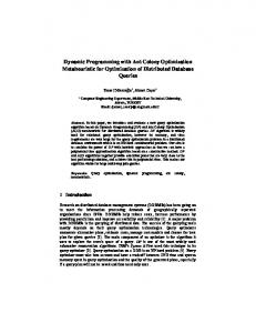
The experiments conducted by Vittori et al. [3], at the CRCA laboratory on the Argentine ant Linepithema humile (previously known as Iridomyrmex humilis) had the objective of monitoring foraging ants within a complex, confined and dynamic environment, so that results would support the model of the insects’ behavior. They consisted of observations of the foraging activities of ants, when a network, comprising branches and bifurcations, is placed between the food source and the ants nest. The network apparatus, Figure 1, consists of four hexagons connected, at angles of 60◦ between two divergent branches. For instance, branches 1 and 4, or 7 and 10. The food source was placed in one of the circular areas A or B, but, due to the symmetry, no differences in the results were observed when either circle was used. There were no experiments with food sources placed simultaneously in both areas. An ant could reach a food source by choosing one among fourteen different paths. Table 1 shows the lengths of the nest-food paths when the food is placed in A. The paths are classified by length: short, medium, long or very long. If an ant passes two or more times along the same branch or does not reach the food source, then this invalid path is classified as a “loop”. The ants behavior was observed and analyzed at two different levels: (i) the collective level, where it was observed if the which path the colonies chose to reach the food and then bring it to the nest, taking into account the lengths of the chosen paths, and; (ii) the individual level, where characteristics such as velocity, number of contacts among the insects, duration of contacts, U-turns2 and time spent at the food source were measured.
3) The access to the food source was allowed only through a long path for 30min, being 1-10-7-5-9-11-3a-13 in case of food source A and 4-7-10-2-11-9-6a-16, in case of food source B. After 30min, the access was allowed to all branches and observation lasts for another 30min.
2.1 2.1.1
Experimental Results Individual Behavior
The individual behavior of the ants was observed with regard to: (i) velocity on the network; (ii) number of contacts with fellow ants; (iii) duration of these contacts; (iv) time spent at the food source, and; (v) number of U-turns on the branches. These data were collected during the first experimental situation, with the static environment [4]. The values observed supported the model.
2.1.2
Collective Behavior
Collective behavior deals with ants individual decisions made under the influence of other ants previous attitudes. This is the origin of self-organized patterns in social insects colonies and plays a very important role in the modeling process. How ants recruit and select path are the major collective features analyzed for the three experimental situations.
Situation 1 – Static Environment with free access When the ants are allowed to freely choose any branch at any bifurcation, 8 in a group of 10 colonies departing from the nest towards the food source direction opted for a short route. From the food to the nest, all the colonies chose one of the shortest paths. Another important component of the ants behavior considered during the experiments, was their recruitment dynamics which consists of the number of ants entering the environment computed at each 3min, in both directions (NestFood and Food-Nest).
Figure 1: Experimental Device.
Three situations were analyzed during the experiments (details in [3, 4, 5]): 1) Ants are allowed to access all branches in the network for 60min; 2) Ants are allowed to access all branches in the network for 30min then, access to the branch which conducts the ants to the food source (3a or 6a), as seen in Figure 1, is blocked and observation lasted for more 30min.
Situation 2 – Blocking a Branch In the second situation, an access to branch 3a or 6a, depending on the position of the food source, was blocked 30 minutes after experiments began and kept inaccessible for the remaining 30 minutes. In this case, there were no short paths, and the medium ones became the shortest routes.
2 Direction change (180◦ ) of an ant within a branch, turning back to their previous location.
170
In the last half, three colonies did not find another route to the food source, these being characterized as loops. Four colonies selected a medium path (the shortest option available) and three chose a long route to reach the food.
a term related to the inclination of the of the branches i and j with the x horizontal axis: Pi (i, j, k) =
Situation 3 – Releasing Blocked Branch
Pipher (i, j, k) = Pidir (i, j) =
MODELING ANT BEHAVIOR
Previous Ant Behavior Model
3.1.5
The first model considered by Vittori, et al. [3, 5] , showed the following properties:
3.1.1
Recruitment Model
1 φmax
(1)
3.2
(2)
where ε ∼ N (0, Vo /10). N represents a normal distribution and Vo is calculated as follows: (3)
being η a constant measured in the experiments and ζ ∼ U [0; ι], where ι is estimated from laboratory measurements.
3.1.3 Pheromone Laying and Evaporation As to the laying and evaporation of pheromone, the model considered the ants laying a quantity fl in the extremities of each traversed branch l. The quantity of pheromone Ql gradually decreases through the parameter δ, 0 ≤ δ < 1: Ql [k] = δQl [k − 1]
3.1.4
Ant Behavior Model - Version 2
As mentioned in the previous subsection, the first model proposed did not reproduce the ants behavior satisfactorily in the three situations. It showed a large number of loops and choices for long and very long paths, but this was not observed in the experiments. The second version of the model [4] was also based on the individual and has the following characteristics: (i) generation of ants at each second (time step); (ii) the ants displacement through the environment; (iii) the ants’ choice at each bifurcation; (iv) the pheromone deposit over the branch traversed; (v) the time spent by each ant at period spent by each ant at the food source, and; (vi)the time the ants kept at a standstill when a branch was blocked. Two characteristics were suppressed in the model: i) Uturns, which were considered negligible, and; (ii) Pheromone evaporation, considered irrelevant due to the relatively short duration of the experiments (60min) compared with the permanence (about 30min) of pheromone after the time it is deposited [7].
The distance traversed by an ant o at each step k was estimated as a velocity component Vo added to a random error ε:
Vo = η + ζ
(8)
where: χ ∼ N (0, κ/µ) is a random error and κ, µ are constants empirically obtained. The values of the constants and further details can be obtained in Vittori, et al. [3, 4, 5]. This model obtained encouraging results for the first experimental situation, with the static environment. However, the second and especially third situations gave poor results [5].
Movement of Ants
Do [k] = (Vo + ε)
(7)
Food Source Delay
Tso [k] = (κ + χ)
where φmax is the maximum number of ants allowed in the experiments (measured as 100 ants on average).
3.1.2
(cosθ)α (cosθ)α + (cosω)α
(6)
The time Tso [k] spent by an ant o at a food source was modeled as
The probability of an ant o entering the environment each time at step k (each second) is: o Pent [k] =
(σ + Qi )β (σ + Qi )β (σ + Qj )β
where θ is the angle formed by the branch i with the axis x; ω is the angle formed by the branch j with the axis x; ρ, τ , σ, α and β are constants empirically obtained. This model also considered a probability that ants could make a U-turn, and come back, inverting their direction along a chosen branch l. This function was represented as a probability depending on the concentration of pheromone deposited in l, the length of l and other empirical constants. In this paper we did not explore such a function. For details see [5].
A first model for the ants behavior, based on the experiments discussed above was proposed by Vittori et al. [3, 4, 5]. The main features are presented in the following subsections.
3.1
(5)
where:
In the first 30 minutes of the third situation, colonies had access only to a long path. Depending on the colony the path was 4-7-10-2-11-9-6a-16 or 1-10-7-5-9-11-3a-13, (Figure 1). After that, the blocks were released and the movement along the paths was allowed. Observations for a further 30 minutes showed that, despite some colonies having kept to the branches previously chosen, most of them succeeded in choosing one of the shortest routes.
3.
ρPipher (i, j, k) + τ Pidir (i, j) ρ+τ
(4)
3.2.1
Path Choosing
Ants Recruitment
The model proposed for the dynamics of the flow of ants F [k] entering the foraging area is:
Two factors were considered in the ants decision to choose a branch in a bifurcation. The probability Pi (i, j, k) of choosing the branch i when the ant is at bifurcation i − j at time step k has two components: (i) Pipher (i, j, k), a term related with the pheromone concentration, and; (ii) Pidir (i, j),
µ ¶ dF [k] F [k] = υF [k] + 1 − dk K
171
(9)
where υ stands for the recruitment rate and K represents the value of the flow at saturation, which is related to the number of foragers available for recruitment within the colony. Integrating the Eq. 9, the ants flow F [k] entering the environment is obtained. Fmax
F [k] =
µ 1+
¶ −k Fmax −1 e τ F0
It was considered that the pheromone amount over an specific branch should be proportional to the number of ants that have traversed it, as proposed by Deneubourg (1990)[7], when modeling the ants behavior.
3.2.5
(10)
B = Baver + ∂Υ
where: Fmax is the maximum flux at the entrance of the network (Fmax = K); F0 is the initial flux at the entrance of the network (F0 = K/(1 + p)); p is a constant; k is the time step related with the recruitment of ants. The values of Fmax , F0 and t were estimated through logistic regression. The value F0 represents the number of ants that initially entered the environment. At each time step k in the simulation, an ant i is recruited with probability Pger [k]: Pger [k] = F [k]
3.2.6
(11)
The velocity of an ant is defined at the instant k it chooses a new branch to move across it. That is, an ant may have variable velocity along its displacement. The velocity is based on the average velocity of the insects in the experiments (Vaver ) and its average standard deviation (Θ): (12)
where: V [k] represents the velocity of the ant at the instant k and ξ ∼ N (0; 1). Consequently the distance traversed between times k − 1 and k is (Eq. 13):
rpref = κ120◦ /κ30◦
(13)
Time Spent on Food Source
The time Ts [k] spent at a food source was modeled by a logarithmic distribution, with a characteristic time (Ξ), obtained in the experiments. The instant k is the time step when the ant reaches the food source. Ts [k] = Ξlog(Z)
Pi =
(κi + Ci )n = 1 − Pj (κi + Ci )n + (κj + Cj )n
(17)
where Pi and Pj represent the probabilities of the ants choosing the branch i or j, respectively; Ci is the concentration of pheromone of the branch i; Cj is the concentration of pheromone of the branch j, and; n is a given constant; Substituting κ120◦ for rpref κ30◦ in Eq.17, and using the best values obtained empirically in the simulations κ = 20 and n = 4, we have:
(14)
Where: Z ∼ U [0; 1], and U represents a uniform probability function with limits 0 and 1.
3.2.4
(16)
For a symmetric bifurcation the intrinsic attraction degree of the branches are equal, κi = κj = κ. For asymmetric bifurcations κ120◦ = κ30◦ rpref . The most common equation used to represent the probabilistic choice of a branch was considered [7, 1]. When an ant reaches the bifurcation i−j, the probability that governs the choice of the next branches is:
where: ∆[k] = is the sampling time (1s).
3.2.3
Path Choosing
In the first model, the orientation of the branches was represented by the angle between the branch and the x axis. However, the angle between the branch of precedence and the candidates for subsequent branches was considered more appropriate. Then two types of bifurcation were distinguished: (i) symmetrical bifurcations, where both branches have a 30◦ angle with the previous trajectory, or; (ii) asymmetrical, where one has a 30◦ angle with the preceding path and the other having a 120◦ angle. In asymmetrical bifurcation, the ants’ choices of the ants in a pheromone free platform (the passage of the first 10 ants in each experiment) were considered in order to estimate the influence of the geometry. From 350 ants observed, 270 opted for the branch with the 30◦ angle, which means 77% of the total choices. We represent the intrinsic attraction degree of the candidate branch i in the absence of pheromone as κi ; if i has a 30◦ angle with the previous branch l, κi = κ30◦ = κ, and if i has a 120◦ angle with l, then κi = κ120◦ = κrpref , i.e., rpref is the decaying of κ for the branch with bigger angle.
3.2.2 The Movement of Ants
D[k] = V [k]∆[k]
(15)
where: B is the delay of the ant; Baver is the average delay, and; ∂ represents the standard-deviation, both empirically obtained, and; Υ ∼ U [0; 1].
where: F [k] is the flux of ants entering the environment at instant k (Eq. 10). In Eq. 11, the generation of an ant i over the environment at k depends on the generation of a random value with uniform probability distribution function. If the number generated is between 0 and the value of F [k], a new ant enters the environment at k.
V [k] = Vaver + Θξ
Blocked Branch Delay
The delay of the ants in the blocked branches (experimental situation 2), was also modeled in the Eq. 15:
Pheromone Deposit
The pheromone concentration in a branch l is initially set to Fin l = 0. When the ants cross the branches, the incremental value q is deposited in each branch in the direction nest-food source, and Q in the opposite direction. In this model, the best results were obtained when the ratio Q/q is set to the unit value 1, Q/q = 1.
r rpref =
4
1 −1 p
(18)
where p = 0.77 is the proportion of ants choosing the 30◦ angle in experiments, resulting rpref = 0.74.
172
The results of this model improved with the modifications above, although several difficulties remained for a changing environment[3]. Such difficulties were associated mostly with pheromone stagnation, i.e., in the second half of the simulations, ants tend to follow the same branches as in the first, due to the bias from pheromone high concentrations. Afterwards, an improvement was tried by incorporating the Metropolis Criterion [8] into the model[5]. Thus, the ants’ choice at bifurcations could be modified. On reaching the bifurcation i−j, coming from the branch l, the ant selects the branch i or j (Eq.17). Then the probability of taking a random decision, different from the first choice, is calculated. Suppose that branch i was chosen, the probability Prand [k] of the ant choosing the opposite branch, j is: Prand [k] = exp (
Ωi [k] − Ωmax ) Γ[k]
response to pheromone concentration. Due to the many difficulties involved in separating these two components, these models include the limitations of ants’ pheromone sensors as well as the influences of pheromone concentrations on ants’ decisions, undistinguished, in the same function. Within the scope of decisions affected by the perceiving pheromone is the deposit of pheromone and following the. Ants’ sensorial system needs a minimal pheromone concentration to influence their decisions [12]. Similarly, a saturation level seems to be biologically plausible. Based on such premises, the constant rate for the pheromone deposit and linear perception were substituted by a sigmoidal model. As we preserved the model for choosing a path based on pheromone concentrations, the deposit rates now depend on the existing amount of pheromone. Such improvement is already well known in the literature [12]. This allows the representation of the saturation effect in the perception by means of limiting the pheromone deposit and simultaneously including the influence of the intensity of pheromone perceived on the trail following decision. Thus, the difference in the degree of preference between the most chosen path and any other path is reduced. This avoids an extremely dominant path situation that leads to stagnation. The pheromone concentration is:
(19)
where: Ωi [k] represents the flux of ants in the branch i until the instant k; Ωmax represents the maximum flux of ants over the branches, and; Γ[k] is the factor responsible for the exploration level of the choices at the time step k. The value of Ωmax was obtained calculating the average of a ten-colony flux of ants at all the branches after one hour of experiments. The variable Γ[k] received the value Ωmax at the beginning of the simulations, empirically obtained. The variable Γ[k] decreases when an ant reaches the food source or the nest: Γ[k + 1] = ΛΓ[k]
Φi [k + 1] = Φi [k] + ε(∆Φ[k])
where: Φi [k] represents the deposited pheromone amount in a branch i at instant k, 0 ≤ ε ≤ 1, and a maximum limit amount of pheromone Φmax in each branch is defined.
(20)
½
where: k = instant when the ant reaches the food source or the nest; Λ = decaying factor of Γ[k] , empirically (0.5 < Λ < 1). It is important to note that Γ[k] was defined as a global variable and thus violates the principles of ACO and selforganization [5]. Anyway, Metropolis Criterion as shown above did not improve the results enough and stagnation remained a problem for dynamic situations.
3.3
∆Φ[k] =
3.3.2
Φmax − Φi [k], 0,
if Φmax ≥ Φi [k]; otherwise.
(22)
Pheromone Evaporation
In the second version of the Ant Behavior Model, the length of the experiment (30–60 min) was considered too short to produce significant evaporation [7], then it was ignored. However, evaporation of more volatile components of pheromone, and influences of substrate and air speed may influence how ants perceive pheromone. Moreover, chemical recruiting in Linepithema humile, under laboratory conditions, may be effaced for about 30 to 60 min [13, 14, 15], and consequently the evaporation effect is possibly relevant. Jeanson, Ratnieks and Deneubourg [14] pointed out that the half-life time to the pheromone of the ant M. pharaonis is about 9 min on a plastic substrate and 3 min on paper substrate. The pheromone duration of M. pharaonis is supposed to be similar to the Linepithema humile due to the wandering behavior they have in common. Both species present opportunistic nesting and probably benefit from the short duration of their pheromone. In spite of this, the presence of long-term components in their pheromone shall not be discarded [16]. In Sol´e et al. [17], for a given evaporation rate, low deposit rates of pheromone lead to more flexibility, which is specially useful when dealing with small and scattered food sources. They also consider a saturation level for the pheromone (Φmax ), and the evaporation decay as in Eq. 23.
Ant Colony Foraging into Dynamic and Confined Model – ACF-DCM
Once the pheromone stagnation was diagnosed as the main problem in former models, the research was directed to investigate the major factors that contributed to that. The Metropolis criterion, previously implemented, was not sufficient to reproduce the random behavior of natural ants and their capacity to adapt. The ACF-DCM results from several modifications in the previous models, with the objective of minimizing the stagnation problems and accurately reproducing the experiments.
3.3.1
(21)
Limiting and Smoothing the Pheromone Concentration
Previous models consider that ants deposit pheromone at constant rates when they traverse the branches. They did not consider either limitations in ants’ perception of pheromone concentrations or the influences of this perception on ants decisions. On this subject, Keshet et al.[9] introduced the concept of an ants’ fidelity to a specific trail: the probability that an ant continues to follow the same branch, and that this varies linearly with the pheromone concentration, until a saturation level is reached. Myerscough et al. [10] formulated a non-linear model for ants’ detection of and
Φi [k + 1] = Φi [k]γ being Φi > Φmin and γ a constant, 0.92 ≤ γ ≤ 1.
173
(23)
Halloy, et al. [18] also consider the evaporation proportionally to the pheromone concentration. The Eq. 23, as used in the ACF-DCM, is well established in the literature [12], above all, for its simplicity. The best simulation results were obtained when a subtle evaporation rate (γ ≈ 0.98) was used.
3.3.3
Table 2: Table of new parameters Function Parameter Value Origin Generation Fmax 0.42/s of Ants F0 5x10⁻⁴ s Estimated τ 127.4s from Branch κ 20 experiments choice n 4 rpref 0.74 Delay on Baver 100s blocked branch ∂ 2.09s Velocity Vaver 1.06cm/s Measured Θ 0.34 in the Ξ 179.9s experiments Time spent Pheromone ε 0.05 deposit Φmax 100 Φmin 5 Empirical Evaporation γ 0.98 values Metropolis Γ 0.98 Criterion Ωmax 10
Metropolis Criterion Modification: Crowding Condition
The Metropolis criterion as used in the previous model presupposes that ants evaluate the cumulative traffic in each branch, and such perceptions influence their decisions, leading them to diverge from their ’deterministic’ choices – based on the pheromone concentration and the geometry of the bifurcation (Eq. 17). Such mechanism made the ants in the first experimental situation correctly avoid very-dominant paths, and helped the model to reproduce real ant behavior. However, for the second and third situations, the simple perception of traffic flow did not suffice to reproduce correctly the behavior observed in experiments. There is a subtle but important difference between the perception of the flow of ants and the perception of the number of ants within a determined branch at a given instant, being stopped or in movement. If a branch has been blocked, the ants stop within it and wait before turning back, as observed in experiments (Eq. 15). Even if the ant flow (Ωi [k]) in this branch i is not altered, a little crowding occurs. Another difficulty observed in the previous model was caused by computing the flow of ants. This requires a time interval in which a certain number of ants will pass through the branch. Vittori et al. [3] employed the total number of ants that have traversed the branch until the instant of calculation. In this case, there is a tendency for the cumulative effect to surpass the recent flow effect, and stagnation may occur. The supposition that the ants are capable of visually detecting agglomerations has strong support in the literature [19, 16, 20], reinforcing the importance of visual cues and avoidance of crowding in foraging ants. The equation used in ACF-DCM is quite similar to Eq.19 used in the previous model, except for the meaning of its variables:
were tested, being γ = 0.98 being the value that gave best results. For Metropolis Criterion parameters, Ωmax was firstly estimated based on the maximum number of ants in simulations without the Metropolis Criterion, while Γ was set empirically by trial and error.
4. RESULTS The implementation of ACF-DCM in ANSI C allowed analysis of the influence of parameters influence over simulations of the three experimental situations. Results were computed to allow comparison with experimental measurements as well as the dynamic of ant colonies The main results are described below.
4.1
Results for Experimental Situation 1
While the previous models have already shown good results for the first experimental situation, ACF-DCM showed even better ones, as they very accurately reproduced the measurements collected in the laboratory with real ants, as illustrated in Figure 2.
Ω[k] − Ωmax ) (24) Γ where Γ is a constant curve parameter, to regulate its smoothing; Ω[k] is the number of ants within the chosen branch at time step k, and; Ωmax indicates the maximum number of ants above which the ants certainly will avoid the agglomeration. The value of Ωmax shall depend on the capacity of the branch, i.e., the narrower is the branch, the lower is Ωmax . In this study, all the branches have the same thickness, thus the same Ωmax . ϕCrowd = exp (
4.2
Results for Experimental Situation 2
Before the branch 3a (or 6a) is blocked, at time step k = 1800, ants obviously behave similarly to situation 1, i.e., they take the shortest paths. After the blockade, several ants take invalid routes, until gradually they find medium routes (the shortest available) and cease the loops, as depicted in Figure 3(a). The ACF-DCM reproduces such behavior very precisely, despite there being a minor deficiency in replicating the number of ants that take a long route. In the reverse direction, food-nest, a minor discrepancy is observed for very long routes, as illustrated in Figure 3(b).
3.3.4 New Parameters Table 2 shows the parameters used in the successful simulations of ACF-DCM. Some parameters could not be measured or estimated from experiments and were empirically set. Pheromone parameters were set empirically to avoid stagnation, i.e, values should not allow branches to have higher discrepancies on pheromone deposited during simulation time, which would make adaption difficult. First, deposit parameters were set, then several evaporation rates
4.3
Results for Experimental Situation 3
The ACF-DCM, differently from previous models, reproduced the ants’ behavior observed in the laboratory, see Figure 4(a), although small discrepancies still remain. After unblocking (30min) it is possible to observe in the simulations that no stagnation occurs. The ants that were previously foraging through a long route, learn and redistribute them-
174
(a)
(a)
(b)
(b)
Figure 2: Choice frequency for the two previous versions of the model, for ACF-DCM and for the experiments, for situation 1, in (a) for nest-food direction and (b), food-nest.
Figure 3: Choice frequency for the three versions of the model and for the experiments, for situation 2, in (a) direction nest-food and (b) food-nest.
selves into medium paths, short paths and loops. As time goes by, the ants migrate to the shortest paths until the end of the simulations. Such observations are quite similar in experiments, besides which real ants still present lower loop rates. In the food-nest direction, simulations also showed good results, as shows Figure 4(b) shows. Here, real ants display a curious behavior. After unblocking, there is a reduction in the occurrence of long routes, but the ants start choosing long paths again in the last 15 minutes of experiments. This behavior was not completely reproduced by the simulations.
haviors of the foraging ants were considered in the model. The choices of the shortest routes were observed in the simulations exactly as in the experiments, when access to the fourteen different paths was allowed (situation 1). When dealing with a dynamic environment, the new model overcomes the stagnation problem, diagnosed as being the main problem in the previous models. This shows how the ants adapt to blocked or unblocked branches (situation 2 and 3 respectively). Three important new elements were introduced in the ACF-DCM: (i) Smoothing and Saturation in the perception and deposit of pheromone. Indeed, introducing these very natural and simple non-linearities are responsible for greatly modeling improving the model; (ii) Evaporation, which helps the model to avoid stagnation. This reflects one of the most important features of real ants, above all, those dependent on scattered food sources and which have to cope with a changing foraging area, and; (iii) Modifying the Metropolis Criterion, by considering the ants’ perception of crowding, which enabled them to avoid crowded branches. This new feature considers ants have little visual capability, which is necessary to perceive agglomerations and then, probably choose an alternative way.
5.
CONCLUSIONS
In the laboratory, foraging ants exhibited their amazing capacities for self-organization and adapting, by finding the best routes in a relatively complex environment and adapting themselves to environmental changes. Such achievements result from the superposition of relatively simple individual behavioral rules. ACF-DCM succeeded in the replicating several behavioral features observed in experiments with the argentine ant Linepithema humile. The simulations reproduce patterns observed in real ants when foraging into confined and dynamic environment. Both the individual and the collective characteristic be-
175
[6]
[7]
[8]
[9] (a)
[10]
[11]
[12]
[13] (b)
Figure 4: Choice frequency for the three versions of the model and for the experiments, for situation 3, in the (a) direction nest-food and (b) food-nest.
[14]
[15]
ACF-DCM has shown to be efficacious at reproducing accurately natural ant colony behavior in a confined and dynamic network, overcoming stagnation problem and increasing biological plausibility. Work is now in progress to evaluate the introduction of other ants sensorial capacities in the model and to explore their possible applications.
6.
[16]
[17]
REFERENCES
[1] E. Bonabeau, M. Dorigo and G. Theraulaz. Swarm Intelligence: From Natural to Artificial Systems Oxford University Press, New York, 1999. [2] J. Kennedy, R. C. Eberhart and Y. Shi. Swarm Intelligence Morgan Kaufmann Press, 1999. [3] K. Vittori, G. Talbot, J. Gautrais, V. Fourcassi´e, A. F. R. Ara´ ujo and G. Theraulaz. Path efficiency of ant foraging trails in an artificial network Journal of Theoretical Biology, 239:507 – 515, 2006. ujo, V. Fourcassi´e, [4] K. Vittori, J. Gautrais, A. F. R. Ara´ and G. Theraulaz. Modeling ants behavior under a variable environment 4th International Workshop on Ant Colony Optimization and Swarm Intelligence, by Marco Dorigo, Springer:190 – 202, 2004. [5] K. Vittori. Experimental Study, Modeling and Implementation of Ant Colony Behavior in a Dynamic Environment. Doctoral Thesis - Escola de Engenharia
[18]
[19]
[20]
176
de S˜ ao Carlos, Universidade de S˜ ao Paulo, S˜ ao Carlos, S˜ ao Paulo, Brazil, 2005. C. Blum. Ant Colony optimization: Introduction and recent trends Physics of Life Reviews, 2:353 – 373, 2005. J. L. Deneubourg, S. Aron, S. Goss and J. M. Pasteels. The self-organizing exploratory pattern of the argentine ant. Journal of Insect Behavior, 3(2):158 – 168, 1990. N. Metropolis, A. W. Rosenbluth, M. N. Rosenbluth and A. H. Teller. Equation of State Calculations by Fast Computing Machines The Journal of Chemical Physics, 21(6):1087 – 1092, 1953. J. Watmough and L. Edelstein-Keshet. Modelling the formation of trail networks by foraging ants. J. theor. Biol., 176:357 – 371, 1995. A. D. Vincent and M. R. Myerscough. The effect of a non-uniform turning kernel on ant trail morphology. J. Mathematical Biology, 49:391 – 432, 2004. D. R. Chialvo and M. M. Millonas. How swarms build cognitive maps. The Biology and Technology of Intelligent Autonomous Agents, Nato ASI Series, Luc Steel 144: 439 – 450, 1995. K. M. Sim and W. H. Sun. Ant Colony optimization for Routing and Load-Balancing: Survey and New Directions IEEE Transactions on Systems, Man and Cybernetics, Part A: Systems and Humans, Vol. 33, 5:560 – 572, 2003. D. Demolin, J. L. Deneubourg S. C. Nicolis, C. Detrain. Optimality of collective choices: A stochastic approach. Bulletin of Mathematical Biology, 65:795 – 808, 2003. F. L. W. Ratnieks, J. L. Deneubourg and R. Jeanson. Pheromone trail decay rates on different substrates in ˇ ant, monomorium pharaonis. the pharaohSs Physiological Entomology, 28:192 – 198, 2003. S. E. V. V. Key & T. C. Baker. Trail-following responses of the argentine ant, Iridomyrmex humilis (mayr), to a synthetic trail pheromone component and analogs. Journal of Chemical Ecology, 8:1 – 14, 1982. B. H¨ olldobler. Multimodal signals in ant communication. J. Comp. Physiol. A, 184:129 – 141, 1999. R. V. Sol´e, E. Bonabeau., J. Delgado, P. Fern´ andez and J. Mar´ın. Pattern formation and optimization in army ant raids. Artificial Life, 6(3):219 – 226, 2000. J. Halloy, J. L. Deneubourg, J. Millor and J. M. Ame. Individual discrimination capability and collective decision-making. Journal of Theoretical Biology, 239:313 – 323, 2006. T. S. Collet. Insect navigation en route to the goal: Multiple strategies for the use of landmarks. The Journal of Experimental Biology, 199:227 – 235, 1996. I. D. Couzin and N. R. Franks. Self-organized lane formation and optimized traffic flow in army ants. Proc. Royal Soc. London – B, DOI 10.1098 rspb.2002.2210:02PB0606: 1 – 8, 2002.