Modeling auditory coding: from sound to spikes - Springer Link
Recommend Documents
miniature head-fixed video camera on the one hand, and to headphones on the other hand. In a second application, called acoustic screen, this sound board is ...
{ingrid.johnsrude,matt.davis,alexis.hervais-adelman}@mrc-cbu.cam.ac.uk. 1 Introduction. Cognitive models of spoken language comprehension postulate ...
judged to move in the direction opposite to that of the adaptation stimulus. We call ... effect is weaker than the visual analog, the data suggest that auditory motion ... tion aftereffects is based on the presumed existence ... cording to this view,
dominance and early experience upon mate selection in male. Convict cichlids, Cichlasoma nigrofasciatum Gunther (Pisces,. Cichlidae). Behaviour, 1975,56 ...
Stretch Coding and Block Coding: Two New Strategies to Represent. Questionably Aligned DNA Sequences. Daniel L. Geiger. Research Associate, Santa ...
access conflicts with ownership rights and ethical issues. It describes two ..... process of Search Engine Optimization in order to identify the informants' names.
study N. meningitidis metabolism as a whole, or certain aspects of it, and it can also be used for ...... acid (Neu5Ac) is synthesized from N-acetylmannosamine.
Tyrrel Road, Millbrook, New York 12545. ' procedure have been reported ..... the New York Academy of Sciences, 1969. 68. 186-198. Davis. H .⢠Bowers.
Sep 26, 2009 - pieces of DNA were often taken for the genes themselves, ... Theory Biosci. ... alternative developed by Prohaska and Stadler between a ... molecular aspects, and not arrive at what makes a cell a ... of structure contributes to a gene
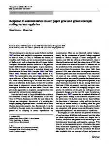
Abstract. Quinlan and Rivest have suggested a decision-tree inference method using the Minimum Description. Length idea. We show that there is an error in ...
Feb 22, 2013 - Some specific forms of auditory perception such as speech perception are often assumed ... Expert radiologists can look at an X-ray and see vague gray scale shapes as ...... Effects of intelligibility on working memory demand.
the source position, directivity and multi-microphone recordings. The acoustic signal emitted by the source is assumed to be broadband, such as a down-swept ...
sounds. Activity in pSTG/MTG had an onset of 150 ms and increased parametrically ..... in the mind's ear: A PET investigation of musical imagery and perception.
Darker hash marks indicate spike times within the response period, which .... refractory period, which could not have been longer than the 2 msec inter-spike.
informal, formal, programming language-based, graph-based semantics), and .... find no programming languages with dedicated concepts to describe finite.
Aug 24, 2012 - to develop a model to quantify risk of disproportionation, where ... Eli Lilly and Company ... API with a range of base pKa and also solubility.
HOWARD J. KALLMAN, STEPHEN C. HffiTLE, and DENISE DAVIDSON. State University ofNew York, ...... Chicago: Rand McNally. MASSARO, D. W. (1976).
to James K. Walsh, Sleep Disorders Center, Cincinnati General. Hospital, Mont Reid Room 23, 234 Goodman ..... In E. Callaway, P. Tueting, & S. Koslow (Eds.), ...
by a PDP 8/e minicomputer and a Commodore microcomputer and disk units. Procedure. Several measures were taken to facilitate learning of the match-.
Key Words : Paraganglioma, External Auditory Canal. INTRODUCTION. The paraganglia are cells derived from the neural crest and are found widely distributed ...
Apr 17, 2013 - could identify environmental sounds such as a doorbell and telephone ring by the third month of surgery. Improvement in mean performance on ...
pearance of a motorcycle from behind the truck. These two ways have .... ing a visual search task (Blocks 1â5, 80 trials each) and a test- ing phase, in which the ...
Electroencephalogra- phy revealed frequent spikes in the left temporal lobe. ... Key words: auditory hallucination, radiotherapy, necrosis, clonazepam, first-rank ...
Modeling auditory coding: from sound to spikes - Springer Link
Jun 7, 2015 - to zero followed by a slow recovery that might follow an .... model, depending on the task, can be selected to drive mod- .... this is very hard in physiological recordings, as it requires ... and clean speech (no noise added) and plotted for differ- ... ample room for further research to bridge the gap between.
Cell Tissue Res (2015) 361:159–175 DOI 10.1007/s00441-015-2202-z
REVIEW
Modeling auditory coding: from sound to spikes Marek Rudnicki1 · Oliver Schoppe1 · Michael Isik1 · Florian V¨olk1 · Werner Hemmert1
Abstract Models are valuable tools to assess how deeply we understand complex systems: only if we are able to replicate the output of a system based on the function of its subcomponents can we assume that we have probably grasped its principles of operation. On the other hand, discrepancies between model results and measurements reveal gaps in our current knowledge, which can in turn be targeted by matched experiments. Models of the auditory periphery have improved greatly during the last decades, and account for many phenomena observed in experiments. While the cochlea is only partly accessible in experiments, models can extrapolate its behavior without gap from base to apex and with arbitrary input signals. With models we can for example evaluate speech coding with large speech databases, which is not possible experimentally, and models have been tuned to replicate features of the human hearing organ, for which practically no invasive electrophysiological measurements are available. Auditory models have become instrumental in evaluating models of neuronal sound processing in the auditory brainstem and even at higher levels, where they are used to provide realistic input, and finally, models can be used to illustrate how such a complicated system as the inner ear works by visualizing its responses. The big advantage there is that intermediate steps in various domains (mechanical, electrical, and chemical) are available, such that a consistent picture of the evolvement of its output can be drawn. However, it must be kept in mind that no model is able to replicate all physiological characteristics
Department of Electrical and Computer Engineering, Technische Universit¨at M¨unchen, M¨unchen, Germany
(yet) and therefore it is critical to choose the most appropriate model—or models—for every research question. To facilitate this task, this paper not only reviews three recent auditory models, it also introduces a framework that allows researchers to easily switch between models. It also provides uniform evaluation and visualization scripts, which allow for direct comparisons between models. Keywords Cochlea · Models · Review
Introduction Hearing is the perception of sound, a sensory impression generated within the central auditory system. It involves a variety of intertwining functional stages that transform an acoustical pressure wave into sensation. From the point of view of information theory, the most critical stage occurs when the continuous analog sound signal is converted into discrete all-or-nothing nerve action potentials. At this stage, a massive information loss occurs (Wang et al. 2011) and any information not coded by the spike trains of the auditory nerve is lost from further processing. For this reason, the way sound is coded in the inner ear has important implications for its perception: many basic features of inner-ear function like hearing threshold, place coding, and tuning of the basilar membrane have their origin in the inner ear and are conserved in the neuronal stages up to the cortical level. As is true for most complex systems, modeling the function of inner hair cells can be approached from a top-down or a bottom-up perspective (Meddis and Lopez-Poveda 2010) and on very different scales of detail. The top-down view generally treats all processing stages of the auditory system as much as a black box as possible and only tries to project inputs of a unit to its corresponding outputs.
160
They are mostly based on signal-processing methods and represent the phenomenological approach. For example, the vibration of the basilar membrane is commonly modeled with a nonlinear filter bank. While this simplistic approach often yields good results, such models provide limited contribution to understanding actual physiological processes. The bottom-up perspective tries to precisely mimic all relevant physiological processes in detail and to incorporate them into one model. Thus, they may include many more parameters than phenomenological models and the choice of such parameters is critical to the model’s performance. However, they may contribute to understanding the causes of inner hair cell behavior and can be used to challenge new hypotheses. Ideally, phenomenological and bottom-up models should converge. This can be nicely observed in phenomenological models, which are based on signal processing methods such as filters and amplifiers. Even though this approach tries to predict the effective outcome rather than the individual physiological processes, signal filters tend to be broken down to ever smaller stages, often corresponding to functionally distinct biological units. Effectively, this can be interpreted as an increasing consolidation of phenomenological and physiological approaches. This trend might also be beneficial in a broader sense, as such physiologically plausible models can be expanded to incorporate pathological alterations and then may serve as a basis to simulate and understand aspects of hearing impairment (Lopez-Poveda 2013). Moreover, models of the inner ear are essential for bottom-up models of the auditory brainstem and even higher neuronal stages, which are progressing quickly. Auditory models are already covered in excellent reviews, e.g., Lopez-Poveda (2005), and for this reason this review intends to go beyond a description of the current state of modeling. We have created a package for Python programming language called cochlea (Rudnicki and Hemmert 2014), which allows researchers to run and analyze a selection of inner-ear models, which generate auditory nerve spike trains from arbitrary sound signals. This package makes it easy to run different models and to analyze and compare them with the same methods. In chapters 2 and 3 we also exploit the strengths of auditory models and illustrate the principles of auditory coding over the whole length of the hearing organ. This possibility provides an enormous benefit over most physiological recordings, where the hearing organ is only accessible from a single location. In addition, models can incorporate all the steps involved in sound coding, starting from the mechanical vibration of the basilar membrane to the chemical processes involved in the release of synaptic vesicles, where current measurement technology is still missing or severely limited, e.g., in sensitivity and/or temporal resolution.
Cell Tissue Res (2015) 361:159–175
Modeling sound coding The auditory system is usually divided into the peripheral and the central part. Whereas the periphery covers the pathway of the acoustic wave up to the inner hair cells, the central auditory system comprises all stages of neural processing up to the perception of sound. Outer and middle ear Auditory processing starts at the pinna and upper body, which filters incoming sound waves in a direction-specific manner, providing an important cue for sound localization, especially in the median plane (Blauert 1974). The acoustic wave propagates towards the eardrum, where the auditory canal’s λ/4 resonance is responsible for the most sensitive frequency region of hearing between 2 and 4 kHz. At the eardrum, or tympanic membrane, sound is converted into mechanical vibrations, which are coupled via the ossicles to the inner ear or cochlea. While the malleus grows into the rather big tympanic membrane, the stapes is attached to the much smaller oval window, which is the entrance to the cochlea. Due to this difference in size and due to a smaller leverage effect, the middle ear mitigates the different acoustic impedances of air-filled ear canal and fluid-filled cochlea in a frequencyspecific manner. Cochlea The cochlea consists of three cavities: scala tympani and scala media are separated by Reissner’s membrane. Scala media and scala vestibuli are separated by the basilar membrane, on which the organ of Corti is located (compare Fig. 1). The electro-chemical composition of scala media is very special. Unlike scala tympani and scala vestibuli, which contain regular extracellular fluid (perilymph) with high sodium and low potassium concentration, the concentration of these ions is reversed in the scala media.
e
an
br
em
'm
s er
tectorial membrane
stria vascularis
n iss
Re
spiral ligament osseous spiral lamina
IHC
OHC
BM 0.1 mm
Fig. 1 Schematic of the anatomy of the organ of Corti, apical part of the cochlea (modified from Hemmert 2015)
Cell Tissue Res (2015) 361:159–175
Traveling wave and active amplification by outer hair cells As the oval window is driven by the stapes motion, it displaces the fluid in scala vestibuli and a wave propagates along the basilar membrane. This traveling wave was investigated in great detail by Georg von B´ek´esy (1928) in cadaver ears. Figure 2 shows the excitation of the basilar membrane along the whole length of the cochlea at two time instances. The input signal consisted of two pure tones (frequencies: 1 kHz and 5 Hz 50 dB SPL). The motion of the basilar membrane runs from the cochlear base to the apex, which is visualized by plotting the BM motion 9.2 ms after signal onset and 0.1 ms later (dashed line). For the 5-kHz tone, 0.1 ms is equivalent to a 180 degree phase shift, while for the 1-kHz tone, the wave has advanced by 36 degrees. For the high-frequency tone, the apparent traveling distance is much larger, the traveling-wave runs fast in the basal part
0
Distance from apex (mm) 10 15 20 25
5
30
35
0.4 x BM,passive (nm)
a) 0.2
0.1nm
0 -0.2 t 1= 10.0ms
-0.4 apical 20
t 2= 10.1ms
basal
envelope
b) x BM,active (nm)
In addition, it exhibits a large positive potential of about 80 mV relative to scala vestibuli. Both the ionic gradient and potential are actively generated by the stria vascularis (Wangemann 2006). The organ of Corti is a highly specialized sensory organ that translates the motion of the basilar membrane into neural signals. It is covered by the tectorial membrane (Fig. 1). It is composed of a complex, three-dimensional latticed framework of supporting- and sensory cells, the so-called hair cells, which take their name from their mechanosensitive sterocilia (or hair-) bundle. As the motion of the organ of Corti deflects the hair cells’ stereocilia in the radial direction, mechano-electrical transduction channels open, which are large, non-selective cation channels (Corey 2006), a process to which a second-order Boltzmann function fits well. When the transduction channel is open, positive ions are driven by the sum of the cells’ membrane potential and the endocochlear potential into the cell. This transduction current charges the membrane capacity of the hair cells and causes depolarization. While outer hair cells react with a contraction of their cylindrical cell bodies, in inner hair cells depolarization triggers a cascade of electrochemical reactions, which finally elicit action potentials in the auditory nerve fibers synapsing on their soma. More details of the mechanisms involved will be explained in the following sections. The action potentials are propagated to the central nervous system, where the sound perception evolves. The potassium accumulated in the cells can leave without effort through basolateral potassium channels due to the concentration gradient with the extracellular fluid. Therefore, the energy required for the potassium flux into and out of the cell is provided mostly by the stria vascularis.
161
10
10nm
0 -10 -20 0.2
0.5 1 2 5 Characteristic frequency (kHz)
10
Fig. 2 BM displacement for the passive and active traveling wave calculated with the model of Holmberg and Hemmert (2004). Note that the excitation is plotted from apical to basal to achieve increasing CFs from left to right. The traveling wave is running from right to left. The input signal consisted of two pure tones (1 kHz 50 dBSP L and 5 kHz 50 dBSP L ). Motion snapshots were taken 9.2 ms after signal onset and 0.1 ms later (dashed line). Dotted lines indicate the envelope of the traveling wave
of the cochlea and slows down as it travels apically.1 With this mechanism frequencies are separated along the BM: for tones with high frequencies, the traveling wave reaches its maximum (indicated by the envelope, dotted line) basally, for lower frequencies, the peak occurs more apically. When the traveling wave has reached its peak, it decays rapidly. Figure 2 was created using the model of Holmberg and Hemmert (2004), as this is the only model in our review which is based on a traveling-wave model; but even filterbank models, where the filters are not coupled from base to apex generate similar results, because filter delays increase with lower CFs, which also gives the impression of a wave “traveling” from high to low CF filters. The passive traveling wave is by far too shallow to explain the exquisite frequency selectivity observed in the mammalian inner ear. First reports that the basilar membrane might be much sharper tuned under good physiological conditions than observed by von B´ek´esy in cadaver ears came from Rhode (1971), but even after this observation it still took several decades until the insight that this 1A
video of the traveling wave is provided in the complementary materials.
162
sharpening is due to an active mechanical process became generally accepted. Active amplification of the traveling wave was postulated first by Gold (1948) and an active inner-ear model (based on electronic circuits) was built by Zwicker in the 1970s (Zwicker 1986), based on speculations of the origins of the strange nonlinear behavior of the inner ear (Zwicker 1955). The idea of the active cochlear amplifier was strongly supported by the discovery of otoacoustic emissions (Kemp 1978) and outer hair cell electromotility (Brownell et al. 1985; Zenner 1986). Finally, the motor protein in the outer hair cells was sequenced and named Prestin (Zheng et al. 2000) due to its speed (Frank et al. 1999). However, a second force-generating mechanism is located in the mechanoreceptive hair bundles, which can generate spontaneous hair-bundle oscillations and may contribute to nonlinear amplification (Chan and Hudspeth 2005; Hudspeth 2008; review in Ashmore et al. 2010). Prestin is most likely required for active amplification (Dallos et al. 2008), but it might also be that both mechanisms contribute to the observed responses (Meaud and Grosh 2011). To make things even more complicated, it has been found that the tectorial membrane also plays an important role in the active amplification process. When its mechanical properties are altered, mechanical amplification is still present but the width of the tuning curves change (Ghaffari et al. 2007, 2010). Along with physiological findings, more and more elaborate concepts evolved, indicating how the cochlear amplifier might work. While a single OHC injects energy locally into the vibration of the organ of Corti and thus counteracts the friction inherent in fluid motion, a local mechanism is not sufficient to explain the shape of the active responses. It has long been postulated that the amplification process is distributed. When the traveling wave builds up before it reaches its maximum at CF, OHCs augment the vibration in each segment of the partition by altering its effective mechanical impedance (Zweig 1991). The energy of the traveling wave accumulates as it traverses the active region and the integral gain can dramatically exceed the local gain provided by a single OHC (Fisher et al. 2012). Notably, the active amplification is largest at low sound levels and saturates quickly. Therefore, low-level signals are greatly (about 1000-fold!, (Ruggero et al. 2000)) amplified, whereas for high-level sounds, the response converges to the passive traveling wave. This processing provides the required nonlinear compression of the huge acoustic dynamic range (more than 120 dB) to the much more limited range that can be processed by the sensory cells. Along with the physiological findings, more and more elaborate inner-ear models evolved (Olson et al. 2012; Geisler and Sang 1995; Yoon et al. 2011; Verhulst et al. 2012), however, as the underlying mechanisms of the cochlear amplifier are still not fully elucidated, up-to-date purely phenomenological models of the whole inner ear
Cell Tissue Res (2015) 361:159–175
are available. The active traveling wave response in Fig. 2 (lower panel) was again created with the model of Holmberg and Hemmert (2004). As systems with high amplification and local feedback tend to become unstable, this model exploits a trick to achieve numerically stable “amplification”: it adds second-order resonators and modulates their damping coefficients. The advantage of using purely passive resonators is that the model is always stable and thus it can be solved efficiently with arbitrary input signals in the time-domain with wave-digital filters (Strube 1985). To achieve the very high amplification observed in the intact inner ear, one resonator is not sufficient; it would be necessary to modulate its quality factor from one to one thousand, which would entail extremely peaky tuning curves and excessive ringing. Using four resonators in series and modulating their quality factors from one to 10 provided a good compromise between amplification/compression (theoretical maximum: 10.000) and filter bandwidth (Holmberg and Hemmert 2004; Holmberg 2009). We notice these effects when we compare the passive and active traveling wave responses in Fig. 2: the passive wave is shallow, especially its high-frequency slope. Its maximal displacement is only in the range of 0.2 nm and therefore below perception threshold. The maximal amplitude of the active wave exceeds 10 nm and is therefore far above the threshold. In addition, as the effects of amplification are effective only in a narrow region basal to the characteristic location, the supra-threshold excitation remains rather narrow. Only at higher levels, when the passive traveling wave begins to dominate, excitation patterns extend to more basal (highfrequency) regions, a phenomenon which is known from psychoacoustics as upper spread of masking (Zwicker and Feldtkeller 1967; Moore and Glasberg 1987). As the system is highly nonlinear, distortions also occur. The largest one is the cubic distortion product (at 2f1 −f2 ), which causes the response at the 3-kHz characteristic location. The inner hair cells The function of inner hair cells is to perform the mechanoelectrochemical transduction from the deflection of their hair bundle to the release of the neurotransmitter, which excites the auditory nerve. While the tips of the hair bundles of outer hair cells are anchored in the tectorial membrane (compare Fig. 1), the hair bundles of the IHCs are probably driven by fluid forces in the narrow subtectorial space. Viscous fluid forces together with the stiffness of the hair bundles give rise to a first-order high-pass filter (Sellick and Russell 1980; Dallos 1986), but it should also be noted that due to boundary-layer effects, this relationship is even more complex (Freeman and Weiss 1988, 1990). Figure 3 shows a sketch of an IHC and its equivalent electrical circuit. A deflection of the IHC hair bundle in
Cell Tissue Res (2015) 361:159–175
163
Fig. 3 Equivalent electrical circuit of an inner hair cell from LopezPoveda and Eustaquio-Martin 2006
the radial direction (towards the OHC) causes tension on the tip-links and opens the mechano-electrical transduction channels. Given the ion concentrations of endolymph and the large endocochlear potential (Et , about +100 mV), the ion influx is largely attributed to potassium (Zeddies and Siegel 2004), which depolarizes the cell. A deflection into the other direction will close partially open transFig. 4 The transmembrane voltage of inner hair cells for sinusoidal stimuli (figure taken from Lopez-Poveda and Eustaquio-Martin 2006). a Physiological data from the guinea-pig for a 50-ms stimulus (data from Palmer and Russel 1986. b Model data from Lopez-Poveda and Eustaquio-Martin 2006)
a)
ducer channels, but the resulting hyperpolarization is much smaller than the depolarization during excitation (Kros and Crawford 1990). This mechanism works as a half-wave rectifier that saturates for large stereocilia displacements (Lopez-Poveda 2013). Even though this mechanism yields results well in line with physiological data, the approach clearly simplifies the mechanoelectrical transduction. The ion channel dynamics are much more complicated and also depend on ion concentrations. As shown in outer hair cells of rats, particularly calcium flux and diffusion within the stereocilia may modulate transducing ion channels (Beurg et al. 2010). Nevertheless, recent data suggests that features such as adaptation of mechanoelectrical transduction can be modeled without taking calcium currents into account (Peng et al. 2013). In the next step, the receptor current is integrated by the membrane capacitance. This gives rise to a low-pass RCfilter which consists of the sum of the ionic conductances of the IHC and the effective membrane capacity (approximately CB +CA ); its corner frequency is around 1 kHz. Due to this filter, the receptor potential is able to follow the excitation of the stimulus only at low frequencies (Palmer and Russel 1986) (compare also Fig. 4). At high frequencies, the AC amplitude is damped and, due to the asymmetry of the transduction current, a DC component arises, which can surmount the AC component in magnitude. This processing has important consequences for how information is coded for low and high frequencies, which becomes immediately clear when we look how the receptor potential evolves along
EXPERIMENTAL (Palmer & Russell, 1986)
b) MODEL (Lopez-Poveda & Eustaquio-Martin, 2006)
25 mV 30 mV
AC 15 mV 12.5 mV
0
10 20 30 40 50 Time (ms)
60 70
0 10 20 30 40 50 60 70 80 Time (ms)
Receptor potential (mV)
164
Cell Tissue Res (2015) 361:159–175
-35 -40 -45 -50 -55 apical
0.2
0.5 1 2 5 Characteristic frequency (kHz)
10
basal
Fig. 5 Receptor potential of IHCs along the cochlea according to the model of Holmberg and Hemmert (2004), which incorporates an IHC model from Sumner et al. (2002, 2003). Hair bundle motion, derived with a first-order high-pass filter from BM motion, serves as input to the IHC model. The acoustic stimulus consisted of two tones (1 kHz and 5 kHz, same as in Fig. 2). Snapshots were taken 9.2 ms after signal onset and 0.1 ms later (dashed line). Dotted lines indicate the envelope of the receptor potential during the stimulus
the cochlea (see Fig. 5). Where the active basilar membrane displacement is still symmetric (compare Fig. 2), in the receptor potential the depolarizing response is clearly dominating. In the apical part of the cochlea, the receptor potential still has a hyperpolarizing component (this is still slightly apparent in the envelope at the 3-kHz characteristic place). The excitation generated by the 5-kHz tone, however, shows only a depolarization effect. This is clearly visible when we look at the envelope of the receptor potential during the signal (plotted in Fig. 5) and is even more nicely illustrated in the supplemented video (Hemmert 2015): even when the hair bundles are displaced in the direction closing the MET channel, the receptor potential stays depolarized, albeit slightly less than for the excitatory stimulation. This is because the DC component, which builds up during a high-frequency stimulus (compare Fig. 4), does not decay within the closing period of the MET channel, as the membrane’s time constant is longer. Physiological studies in guinea-pigs showed that while the transmembrane voltage tightly follows the stimulus for low frequencies, the DC component grows for increasing frequencies and almost entirely characterizes the voltage for stimuli above 5 kHz (Fig. 4A, (Palmer and Russel 1986)). This limits the hair cell’s ability of phase-locking for higher frequencies. The ratio of the AC and the DC component of the transmembrane voltage were also amplitude-dependent. For low sound levels the ratio grew expansively, but it showed compressive behavior for medium and high sound levels (Patuzzi and Sellick 1983). Generally, the low-pass characteristics of the AC/DC-ratio are qualitatively well matched by model data (Fig. 4B). Also, the quantitative measures such as cut-off frequency (around 1 kHz) and order (first order) are in alignment for a wide range of stimulus ampli-
tudes (Lopez-Poveda and Eustaquio-Martin 2006; Sumner et al. 2002). Other characteristic effects are less well understood. For a constant stimulus, some models predict a slow decrease of the DC component (onset adaptation) and a significant hyperpolarization after stimulus offset that gradually recovers (offset adaptation, Zeddies and Siegel 2004). According to that model, both features are largely caused by the dynamics of slow potassium channels (Zeddies and Siegel 2004). This general notion is supported by physiological studies in vitro in which either slow or fast channels were blocked (Kros and Crawford 1990; LopezPoveda and Eustaquio-Martin 2006). However, this effect could not be reproduced by in vivo recordings, putting the validity into question (Zeddies and Siegel 2004). Possible explanations resolving these contradicting results include potential impalement of the inner hair cell’s membrane during in vivo recording with sharp electrodes. This technique is prone to cause a non-specific leakage, which could change the transmembrane voltage considerably. Introducing such a non-specific conductance into the model caused both features to disappear (Zeddies and Siegel 2004). Taken together, this may indicate that the non-existence of those features could be attributed to the recording method. Whether or not the inner hair cell transmembrane voltage shows a peri-stimulus decay of the DC component and post-stimulus hyperpolarization has not yet been resolved conclusively. Synaptic mechanisms The signal transmission from the inner hair cells to the auditory nerve fibers occurs via so-called ribbon synapses. These synapses are known for being temporally very precise and for providing a very reliable transmission. The neurotransmitters that are to be released into the synaptic cleft are encapsulated in vesicles. These vesicles are stored intracellularly in vicinity to the membrane in a cytomatrix, which forms a reservoir. Recent studies investigated the precise roles of the cytomatrix proteins and how they contribute to storing and releasing vesicles (Wu et al. 2014). Data suggests that Bassoon, one of those proteins, is responsible for storing vesicles and reduced expression of Bassoon leads to reduced readily releasable vesicle pools (Jing et al. 2013). Piccolino, a ribbon synapse specific variant of the cytomatrix protein Piccolo, is known to mediate vesicle processes during exo- and endocytosis (Regus-Leidig et al. 2013). Hair cell ribbon synapses can sustain high rates of vesicle release (Moser et al. 2006a) and are able to synchronize the release of multiple vesicles to produce large AMPAmediated excitatory postsynaptic currents (Glowatzki and Fuchs 2002). The underlying mechanism for multivesicular
Cell Tissue Res (2015) 361:159–175 Fig. 6 Kinetic model of Ca+2 binding followed by vesicle fusion (according to Beutner et al. 2001)
165
Ca2+ 5k
Ca2+ 4k
on
on
Dynamics of vesicle fusion
Fusion rate (1/s)
local [Ca2+]i 2.2 µM 4.6 10.0 21.5 46.4 100.0
100
10
0
on
Ca2+ 2k
on
Ca2+ 1k
on
B(Ca)0 B(Ca)1 B(Ca)2 B(Ca)3 B(Ca)4 B(Ca)5 3 3k b2 5k b4 1koff b0 2koff b1 4k b off off off
release at ribbon synapses is still unknown. Neurotransmitter release from IHCs is triggered by Ca2+ entry that is carried almost exclusively by CaV 1.3 channels. These channels are voltage sensitive and open upon depolarization of the cell membrane. They are clustered at the presynaptic active zones and colocalized with readily releasable vesicles (Graydon et al. 2011). The CaV 1.3 channels open very rapidly following a stimulus with a delay of about 50 μs, the onset time constant is about 0.18 ms (Zampini et al. 2013). Furthermore, the local calcium concentration is the integral of the calcium influx and therefore also has a lowpass characteristic (Kidd and Weiss 1990). Although the molecular identity of the Ca2+ sensor is still not identified, it is highly cooperative, requiring the binding of multiple Ca2+ ions to trigger release (Fig. 6, according to Beutner et al. 2001), resulting in rate constants that are strongly Ca2+ dependent (see Fig. 7, Hemmert et al. 2003). Taking into account that there will always be a certain calcium concentration above zero, it can be assumed that at least some of the binding sites are expected to be already filled with calcium. Transferring this notion to the kinetic model, it can be expected that the model is already in an advanced state and fewer binding sites have to be filled to reach vesicle fusion, which improves the speed of the vesicle fusion with increasing [Ca+2 ]i . In order to reach high calcium concentrations, which are required for fast vesicle fusion, it is essential that
10 -10
Ca2+ 3k
10 Time (ms)
20
30
40
Fig. 7 Kinetics of vesicle fusion shows very strong [Ca+2 ]i dependence, figure from Hemmert et al. 2003
γ
fused
CaV 1.3 channels are in very close proximity to the vesicle release sites (Graydon et al. 2011). As the speed of vesicle fusion depends so strongly on [Ca+2 ]i , Goutman (2012) proposed that resulting vesicular depletion provides a compensatory mechanism to ensure constant synaptic delays. Onset adaptation A fundamental phenomenon observed in all sensory systems is (onset) adaptation. This term describes the widely observed neural reaction to constant stimuli, which is characterized by a very high firing rate at the onset of the stimulus that quickly decays to a much lower (or adapted) rate of firing. The auditory nerve is not an exception and also shows this type of neural response, having far-reaching implications on neural information processing in higher stages of the auditory system (Perez-Gonzalez and Malmierca 2014). For example, the degree of onset adaptation of the firing rate depends on the characteristic frequency of the fiber and thereby contributes to mechanisms for maintaining efficient coding of temporal information such as phase-locking (Sumner and Palmer 2012; Perez-Gonzalez and Malmierca 2014). The typical time course of onset adaptation can be seen in Fig. 8, left panel (arrow heads 1 and 2). Two approaches to modeling the dynamics of neurotransmitter vesicle release have been developed by Westerman and Smith (1988) and Meddis (1986) (Fig. 9). The Westerman approach focuses on implementing a series of three vesicle pools feeding into each other. Each transition is governed by its own time constant, which allows for mimicking observed vesicle dynamics closely. The Meddis approach, in contrast, only has two vesicle pools but therefore also takes endocytosis into account, and is the first vesicle model to do so. Even though both models are structurally different, it was shown that the mathematical description of the resulting vesicle dynamics are closely related (Zhang and Carney 2005). Based on those two fundamental approaches, a series of improvements and refinements thereof have been developed (as reviewed by Meddis and Lopez-Poveda (2010)). Offset adaptation Another important aspect of auditory nerve adaptation is the drop of firing rate well below the spontaneous rate of
166
Cell Tissue Res (2015) 361:159–175 b)
(1) (2) (3)
Time
AN firing rate (spikes/s)
AN firing rate
a)
2000 1500 100 500 0 0
20
40 60 Time (ms)
80
100
Fig. 8 Adaptation of auditory nerve activity for a constant stimulus. a Simplified morphology of the neural response to a constant stimulus (gray bar); the peak response occurs with a small delay after stimulus onset and then decays rapidly with a short time constant (1), which is followed by a longer, sustained decay with a longer time constant (2); after stimulus offset, activity plummets clearly below the spontaneous
rate and - after a dead time - slowly recovers (3); (adapted from Zhang and Carney 2005). b Peri-Stimulus Time Histogram (PSTH) for a constant stimulus of 50 ms duration; gray lines show the recordings of 46 auditory nerve fibers from the ferret at their characteristic frequency at 35-45 dB (SPL); the black line shows the mean value (based on Sumner and Palmer 2012)
the respective fibers after the offset of the stimulus. The term offset adaptation refers to this drop and the recovery back to the pre-stimulus rate of spontaneous firing. It is characterized by a certain dead time of a rate close to zero followed by a slow recovery that might follow an exponential function (arrow head 3 in Fig. 8, left panel). While early models were capable of modeling onset adaptation well, the initial approach to predicting offset adaptation with a single exponential with a time constant in the range of 40 ms to 100 ms failed to reproduce the
dead time (as reviewed by Hewitt and Meddis (1991)). One important aspect to look at is the transmembrane voltage after stimulus offset. As mentioned in “The inner hair cells”, it remains unresolved whether and if so, to what degree the inner hair cell hyperpolarizes after stimulus offset. While in vitro recordings showed significant hyperpolarization (Kros and Crawford 1990), this was not the case for in vivo recordings, which might have been caused by cell membrane impalement (Zeddies and Siegel 2004). However, models that otherwise reproduce physiological data with reasonable
Fig. 9 Two approaches to modeling vesicle release dynamics (figure based on Meddis and Lopez-Poveda 2010). a Model of Westerman and Smith (1988). b Model of Meddis (1986)
Cell Tissue Res (2015) 361:159–175
167
accuracy would also qualitatively predict such a hyperpolarization, albeit with some discrepancies (Zeddies and Siegel 2004; Lopez-Poveda and Eustaquio-Martin 2006). Even though hyperpolarization would be a candidate to explain offset adaptation in auditory nerve fiber firing rate, its role remains unclear. Proven to be a plausible approach to onset adaptation, vesicle dynamics were considered by several studies as a physiological basis for offset adaptation as well. Modeling the availability of vesicles in immediate reservoirs, it can be expected that it takes a certain time after stimulus offset for the readily releasable vesicle to reach pre-stimulus levels (Sumner et al. 2003). Since auditory nerve activity is caused by vesicle release, which in turn is a function of the amount of available vesicles, reservoir replenishment seems like an adequate candidate for explaining and modeling offset adaptation. However, given the single exponential nature of the recovery that would be predicted by such a model, it is structurally incapable of reproducing the aforementioned characteristic dead time of a firing rate close to zero (Sumner et al. 2003). Although it was possible to add offset adaptation in a pool model (Zhang and Carney 2005), this approach predicted firing rates that were in conflict with physiological recordings in certain conditions (Zilany et al. 2009), therefore this approach was replaced by introducing power law adaptation. Power law adaptation When one looks at neuronal responses at different time scales, adaptation time constants at every order of magnitude are observed (Kiang et al. 1965), which challenges pool models. Coming from a phenomenological perspective, the concept of power laws has recently attracted interest for modeling adaptation of neural systems (Drew 2006). Instead of following the exponential approach (r(t) ∝ e−βt ), it assumes a relationship between the rate r(t) and a certain power β of time: r(t) ∝ t β
(1)
Transferring this widely used concept to adaptation leads to a rate that is driven by a stimulus, but indirectly suppresses itself (Drew 2006). In contrast to exponential decays, power law adaptation shows scale-invariant behavior and thus, may be apt to meet the requirements of adaptation on multiple time scales (Zilany et al. 2009), as it is observed in the auditory nerve activity. Most importantly, the concept of power law adaptation is capable of reproducing the characteristic slow recovery of spontaneous firing rate after a certain dead time (Fig. 13) and dynamic range adaptation (Zilany and Carney 2010).
A phenomenological model of the auditory periphery made use of the power law concept of adaptation and integrated the approach into the synapse between inner hair cells and auditory nerve fibers (Zilany et al. 2009). The model successfully reproduced physiological data for onset and offset adaptation. Furthermore, it showed convincing similarity with regard to distribution of firing rates over time. A recent update managed to incorporate the differences in response properties of auditory nerve fibers with different characteristic frequencies (Zilany et al. 2014). However, even though the approach of power law adaptation proved to be capable of reproducing physiological recordings over a wide range of settings and for a wide range of neural response properties, it remains a purely phenomenological one. More specifically, the physiological processes that could serve as a basis for power law behavior are unknown (Zilany et al. 2009). Efferent influences It is noteworthy that synaptic excitation by inner hair cells is not the only input driving auditory nerve fiber activity. Two efferent pathways are known to modulate auditory nerve signaling. While one of them, the medial efferent pathway, acts indirectly by regulating outer hair cell activity, the lateral efferent pathway directly acts upon the synapse between the inner hair cell and the auditory nerve fiber (as reviewed by Meddis and Lopez-Poveda (2010)). However, this direct influence largely remains obscure and thus, is difficult to model. Nevertheless, the efferent innervation might play an important role in dynamic range adaptation (see next section). Generally, direct efferent modulation of the synapse is known to play an important role for synapse formation during development (Sesena et al. 2014; Wedemeyer et al. 2013). A recent study showed that it may also modulate synapse strength during maturity (Fuchs 2014). In contrast, the efferent influences on outer hair cells are much better understood (Guinan Jr 2010). Recent models for auditory nerve activity included the efferent effect of the (binaural) medial olivocochlear reflex and could reproduce characteristic physiological data (Clark et al. 2012; Smalt et al. 2014). Dynamic range adaptation As previously mentioned, the AC/DC ratio of the transmembrane voltage grows expansively for small and compressively for medium to high sound pressure levels (Patuzzi and Sellick 1983). More specifically, both components show saturation for high stereocilia displacements above 100 nm, but different growth slopes for smaller displacements. Model simulations suggest that the compressive transfer function between stereocilia displacement and transmembrane
Dynamic range adaptation
a) b)
300
Unadapted Firing rate
200 100 HSR 0
ΔL
Adapted (level shift ΔL)
a') 300 Sound level
200 100 MSR 0
Firing rate adaptation b')
a'')
ΔR
Unadapted
Adapted (rate shift ΔR)
Firing rate
Firing rate (spikes/s)
Fig. 10 Left panel: auditory nerve firing rate as a function of sound pressure level for high, medium and low spontaneous rate fibers (based on Sumner et al. 2002). Scatter plots show physiological data from Winter et al. 1990, solid lines the prediction by the model. Right panel: conceptual difference between dynamic range adaptation and firing rate adaptation as suggested by Wen et al. (2012)
voltage can be attributed to potassium channels and this compression already occurs before saturation of mechanoelectrical transduction is reached (Lopez-Poveda and Eustaquio-Martin 2006). Coming from a top-down perspective, a very different approach is to analyze auditory nerve activity in terms of firing rate as a function of sound pressure level. While recent studies suggest that auditory nerve fiber activity generally follows a third-order function of the stimulus amplitude (Heil 2014), the precise transfer function for auditory nerve activity is more complex and depends on several aspects. Just like the transmembrane voltage, the so-called rate-level functions exhibit saturating behavior, but they very much depend on the type of auditory nerve fiber of interest (Fig. 10, left panel). By fitting free parameters to the spontaneous rate of a given auditory nerve fiber, model predictions of rate-level functions match physiological data closely (Sumner et al. 2002). The obvious differences of dynamic range for different types of fibers are a fundamental basis for efficiently coding signals in the auditory nerve as a whole, given the limits of dynamic range that can be coded by a single nerve fiber. Another basis for increasing efficiency of coding for a wide dynamic range is dynamic range adaptation. One method to assess changes in coding for natural-like situations of changing dynamic ranges is to use stimuli that vary in their distribution of non-uniform sound pressure levels (as described in Dean et al. 2008 for the midbrain). It has been shown that a model with power-law adaptation is also able to explain the time course of adaptation of the mean firing rate and changes in the dynamic range
80 Sound level
observed in AN responses (Zilany and Carney 2010). A recent study for the auditory nerve revealed that adaptation of the dynamic range occurs simultaneously with firing rate adaptation (Wen et al. 2012). While dynamic range adaptation actually represents a change in coding behavior, firing rate adaptation refers to the well-known concept of decrease of firing rate for ongoing stimuli (Fig. 10, right panel). It could be shown that both types of adaptation roughly occur at the same time scale of 100 ms to 400 ms and that they are interdependent (Wen et al. 2012).
A brief overview of model responses While our knowledge about the function of the cochlea has greatly improved during the last few years, still, many processes have not yet been elucidated in their details. Therefore, models of peripheral auditory processing still have to rely – at least partly – on phenomenological implementations, for example for the active amplification process or for offset adaptation. Many models have been developed and published, which cover parts of the processing in the inner ear, even active traveling-wave models (Verhulst et al. 2012) or elaborate inner hair cell models (LopezPoveda and Eustaquio-Martin 2006; Zeddies and Siegel 2004). Fewer incorporate the whole chain from sound pressure to nerve-action potentials in the primary auditory nerve or even the next neuronal processing steps in the auditory brainstem (reviewed by Lopez-Poveda (2005)). However, published manuscripts provide only a very limited view
Cell Tissue Res (2015) 361:159–175
and they can show only selected responses to which the model was tuned. Quantitative comparisons require identical input sounds and standardized analysis methods. As many models are available online, we have selected three recent ones, and made them and a collection of test scripts available in the python package cochlea (Rudnicki and Hemmert 2014). It provides simple access to the models, as they are treated as black boxes. The input is always a sound-pressure signal (in Pascals), the output are N spike trains of the auditory nerve from a single CF or a range of CFs, where N can be selected independently for high, medium- and low-spontaneous rate fibers (HSR, MSR and LSR fibers). With this package, it becomes easy to use, compare and evaluate these different models. Even more importantly, the spike-trains from the most appropriate model, depending on the task, can be selected to drive models of higher auditory processing. The included models are quite heterogeneous, but all of them were tuned to reproduce human performance. The model of Holmberg et al. (2007) is the only one with an underlying traveling-wave model. Compressive amplification is implemented with four additional, cascaded second-order resonators. It was designed to achieve human-like speech coding with very large mechanical compression/amplification of more than 60 dB. It is complemented with an inner hair cell/auditory nerve model from Sumner et al. (2002). The Matlab Auditory Periphery by Meddis (2014) is the only model in our collection with efferent feedback, that modulates cochlear gain and it also implements many auditory brainstem and even midbrain neurons. The model of Zilany et al. (2014) is the only model with power-law adaptation. It also includes a fractional-Gaussian-noise-driven Poisson process to model long-term changes in rates of AN fibers. The last property was disabled in order to simplify comparison with the two other models.
Fig. 11 Rate thresholds of the three models, which are available in the cochlea package (Rudnicki and Hemmert 2014)
169
Fig. 12 Comparison of rate-tuning curves for two fibers with CFs of 500 Hz (solid lines) and 2 kHz (dashed lines). Peaks and drops in the filter responses are due to nonlinearities in the models
Figure 11 shows the rate thresholds of these models and compares them with the human auditory threshold. Usually, a simple filter, which mimics the middle ear, is used to tweak the frequency-dependence of hearing threshold. While the rate thresholds do not really follow the human hearing threshold, they do not deviate by more than 20 dB in the range from 100 Hz to 8 kHz. Especially at low frequencies they seem to be less sensitive, which is expected, as at low frequencies sounds can probably be detected due to the synchronization of the nerve action potentials even when the firing rate is not yet elevated. Larger differences between the models are apparent in the tuning curves plotted in Fig. 12. Human/primate tuning curves might be sharper than in other mammals (Shera et al. 2002) (although this is debated, see Ruggero and Temchin 2005; Lopez-Poveda and Eustaquio-Martin 2013). The models of Holmberg et al. (2007) and Zilany et al. (2014) have implemented sharper tuning curves compared to the Meddis (2014) model, as they were tuned to the psychoacoustic measurements from Shera et al. (2002). As the Holmberg et al. (2007) model is based on a travelingwave model with four second-order low-pass filters on top, it reaches very steep high-frequency slopes (up to about 200 dB/oct), where the slopes of the other filter-based models are limited due to their lower filter order. The peristimulus time histograms (PSTH) of high spontaneous-rate fibers in Fig. 13 illustrate the adaptation behavior of the modeled fibers. All models showed mostly valid primary-like characteristic as seed for example in Fig. 8. However, we observed a systematic increase of the firing rate every 10 ms in the Meddis (2014) model, probably due to the efferent feedback effect. Note that the model of Zilany et al. (2014) has the option to set fluctuating spontaneous rates, which was disabled here. It showed unusually strong onsets with a notch for the higher frequency stimulus. Offset adaptation is only implemented in Zilany’s
170
Cell Tissue Res (2015) 361:159–175
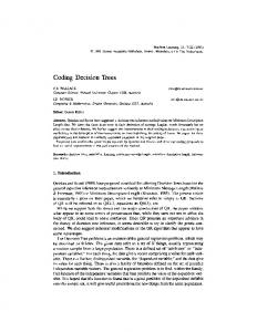
Fig. 13 Peristimulus time histograms (PSTH) of high spontaneous-rate fibers at CF ≈ 2 kHz (in upper panels) and CF ≈ 8 kHz (lower panels). All stimuli were 60 dB above threshold, bin size was 1 ms. For reference data from Sumner and Palmer (2012), see Fig. 8, right panel
phenomenological model. This is not surprising, as the underlying physiological process is still obscure. However, offset adaptation can be very important for further neuronal processing. It was shown that onset type neurons in the auditory brainstem require a short period of silence before a stimulus onset to react to that signal (Wang et al. 2011). Even the spontaneous auditory nerve activity is enough to activate their low-threshold potassium channels, which in turn elevates their firing thresholds. Therefore, if modeled ANF spike trains are used as input to neurons in the brainstem (or even higher), one should consider the Zilany et al. (2014) model or at least use its output for a cross check. The rate-level functions for high-spontaneous rate fibers (Fig. 14) were again quite similar, their dynamic range is in general around 20 dB (Fig. 10). Medium-spontaneous rate fibers exhibit flatter growth functions and larger dynamic ranges. Rates of low-spontaneous rate fibers grew continuously only for the Zilany et al. (2014) model, in the two other models rates stagnate at levels above 70 dB. Here it has to be noted that the rate-level function depends on a delicate interplay between the AC and DC component of the receptor potential, which depends on the dynamic compression of the basilar membrane vibration. Because of relatively large variability of the measured data (e.g., data points in Fig 10), all models reproduce some subset of the experimental data. Phase-locking was analyzed in Fig. 15. The phenomenological model from Zilany et al. (2014) was fit to replicate physiological data, whereas the other two models rely more on the replication of the most important physiological processes involved. Zilany’s model achieved good phaselocking up to high frequencies and the rapid decline of the synchronization index, which was observed in experiments (e.g., data from a cat in Johnson (1980)). This was realized by introducing a fourth-order low-pass. The physiological oriented models that have only implemented the first-order IHC membrane low pass and integrate Ca2+ influx to Ca2+
concentration with a single integration time constant exhibit a more gradual decline. The discrepancy between the physiologically based models and the phenomenological model indicates that further physiological processes probably act as low-pass filters. The next process in synaptic processing, the speed of the CaV 1.3 channels, would be a candidate for additional low-pass filtering. Although Zampini et al. (2013) measured a time constant of about 0.18 ms, although at large IHC depolarization (50 mV), for smaller depolarizations, it might be even longer. Ca2+ binding dynamics required for vesicle fusion is another process, which could provide low-pass filtering. In theory, every binding site could add one filter order. The dynamics of vesicle fusion is not yet included explicitly in inner ear models, which is not surprising, as the underlying mechanisms and time constants are not yet known. Here an interesting feature of physiologically based modeling becomes apparent: if Ca2+ binding dynamics play a significant role in limiting the synchrony at high frequencies, the binding model predicts a speed-up (which means better synchronization) at higher Ca2+ concentration, which might be reached at high sound levels. If the dynamics of Ca2+ binding would be the dominating process, phase-locking might be even faster at high sound levels. Also the modulation gain of the Zilany et al. (2014) model 10 dB above rate threshold was higher compared to the other models (Fig. 16), which might be due to its offset adaptation. The modulation gain also showed a low-pass characteristic, which is – in contrast to phase-locking – also dependent on the filter bandwidth. This is why the point of high-frequency roll-off was lowest for the Holmberg et al. (2007) model, followed by the Zilany et al. (2014) and then the Meddis (2014) model. From physiological recordings (Joris and Yin 1992) it is known that the modulation gain decreases at higher levels.
Cell Tissue Res (2015) 361:159–175
171
Fig. 15 Phase-locking of HRS fibers, measured with the synchronization index, of high spontaneous-rate fibers along the length of the cochlea to pure tones at CF. Sound levels were adjusted 20 dB above the fibers thresholds. Dots indicate physiological data from Johnson (1980)
Fig. 14 Rate-level functions of high-, medium-, and low spontaneousrate fibers at a CF of 8 kHz. Please compare with the data from Winter et al. (1990) provided in Fig. 10
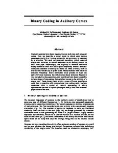
One of the largest benefits of models is the analysis of auditory nerve responses to complex sounds, because this is very hard in physiological recordings, as it requires sampling nerve fibers along the whole CF range of the cochlea. Figure 17 shows averaged firing rates for an artificial vowel “ø”. Voiced speech sounds are generated by glottis vibrations, which generates a fundamental frequency (in our case: 200 Hz) and its higher harmonics (400 Hz, 600 Hz, 800 Hz, ...). This line spectrum is filtered by the vocal tract, which superimposes the characteristic formant structure. The sound was generated with a vocoder with a constant fundamental frequency, which makes it easy to assess the frequency resolution of the models directly from averaged spike counts. The fundamental frequency of the vowel and its harmonics were well resolved in the two models tweaked to human performance at least up to 1 kHz. As the traveling-wave model used in the Holmberg et al. (2007) model was restricted to 100 locations to limit the computational burden, its resolution appears coarse compared to the other models, for which responses at 200 CFs were plotted. The MAP model, due to its broader filters, resolved only the
fundamental frequency, and the second and third harmonics 400 Hz at 600 Hz were scarcely separated. The coarse shape of all response functions was dominated in all cases by the speech formants, F1 at 450 Hz, F2 at 1450 Hz and F3 at 2450 Hz. In the low-frequency range (below 300 Hz), the filters of the Holmberg et al. (2007) model are still very narrow. This model would require structural changes to replicate the low-frequency region of the inner ear more accurately. The Zilany et al. (2014) model does not provide responses for CFs below 125 Hz due to the way it is implemented, that is why response could not be calculated down to 100 Hz in Fig. 17. For the Holmberg et al. (2007) model, MSR and HSR fibers show very similar response curves, while for the Zilany et al. (2014) model, the different fiber types seem to nicely code different dynamic ranges. For the MAP model, the HSR fibers seem to saturate early, despite its smaller overall sensitivity (compare Fig. 11).
Fig. 16 Modulation gain at a CF of 8 kHz for stimuli 10 dB above the individual rate threshold (hearing level, HL) for HRS fibers only. The light gray area represents reference data from Joris and Yin 1992
172
Cell Tissue Res (2015) 361:159–175
and clean speech (no noise added) and plotted for different speech levels in Fig. 18. The MAP model reached the highest recognition scores, despite its relatively broad tuning and limited dynamic range. Obviously, it was able to sustain a very good representation of the speech sounds in noise, which might be attributed to its efferent feedback mechanism. However, its performance was high only at low levels. Already at medium levels (above 40 dB(A)), its performance decayed rapidly, probably because of the saturation of its rate-level functions. The Holmberg model was designed to cover a very broad dynamic range, which is also reflected in the results: the roll-off of recognition scores to low and high levels was shallow. Still, the Zilany et al. (2014) model outperformed the Holmberg et al. (2007) model at all sound levels. This is probably due to the carefully tuned rate-level functions across the whole frequency range, but also offset-adaptation is known to improve speech coding (Wang et al. 2008). In summary, the ability of auditory models to code speech is already very elaborate, all three outperform classical Mel-frequency cepstral features (MFCC), the “gold standard” of automatic speech recognition, which reach a recognition score of 74.8 % (they are level-independent) in the same setting! From these results we can therefore conclude that although auditory models are certainly not perfect yet, they are already powerful tools to provide rather realistic auditory nerve responses. Fig. 17 Comparison of ANF activity for an artificial vowel “ø” at 60 dBSP L (fundamental frequency: 200 Hz, speech formants F1: 450 Hz, F2: 1450 Hz, F3: 2450 Hz). Spike rates were averaged over the vowel duration (400 ms)
Finally, we undertook a very high-level comparison between the models: we wanted to evaluate their discriminative ability to code speech sounds. For a fair comparison, we first equalized their rate thresholds. We decided to match the human hearing threshold, even if this might not be the most optimal setting. Because the auditory models are computationally expensive, we could only use a small speech database, the noisy ISOLET (Holmberg et al. 2007). Acoustic features were extracted from the rate-place coding by summing spikes from HSRs, MSRs and LSRs in overlapping Hanning windows (duration: 25 ms, advanced by 10 ms (Holmberg 2009; Holmberg et al. 2007)). They were preprocessed by a multi-layer perceptron and then fed to a Hidden-Markov speech recognizer. The recognition system was trained and tested for each level individually, because ASR systems are known for their weakness to adapt to previously unseen variations in the feature space. For a detailed description of the system compare Holmberg et al. (2007) and Holmberg (2009). Recognition scores were averaged over the conditions 0, 5, 10, 15, 20 dB SNR
The road ahead: current trends and future work This text reviewed a variety of approaches to modeling inner-ear function. It not only assessed the methods to model the complex interaction of numerous physiological
Fig. 18 Results of an automatic speech recognition system evaluating rate-place code features of the noisy ISOLET database (which contains speech sounds from 0 dB SNR to clean) at different speech levels. Speech recognition scores of the same system with classical Mel-frequency cepstral features was 74.8% (dashed green line)
Cell Tissue Res (2015) 361:159–175
processes, but also qualitatively compared the models’ performance to predict auditory nerve fiber activity with regard to auditory thresholds, temporal coding, dynamic range, adaptation and even speech coding. A major advantage of biologically motivated modeling is that it yields insight into the underlying mechanisms. It can thus be used to come up with hypotheses for specific conditions which can be challenged in physiological experiments. A purely mathematical approach such as present power law adaptation is consequently limited in its application. Nevertheless, it may well serve as a promising basis for unraveling adaptation of auditory nerve fiber activity. The current situation leaves ample room for further research to bridge the gap between mathematical modeling and physiological understanding. One fundamental problem in cochlear modeling is that we still do not have a thorough understanding of the active amplification process in the inner ear and therefore all models rely on artificial mechanical input derived from phenomenological filter models. It is very nice to observe that this gap is closed with nonlinear traveling wave filter models, which will in future hopefully model otoacoustic emissions as well as neuronal responses. This would provide a means to individualize models based on measurement data and hopefully better predict the impact of hearing loss on neuronal coding. Another trend can be observed in a rising number of studies proposing a paradigm shift from lumped-element to spatial modeling. For neurons in general, but also for inner hair cells, spatial and spatiotemporal aspects such as calcium diffusion receive growing attention (Shen and Shuai 2011). For example, it could be shown that detailed diffusion models can be necessary to simulate calcium-driven effects in ion channels in neurons (Anwar et al. 2012). Recent studies emphasize the importance of spatial coupling between calcium influx and exocytosis (Wong et al. 2014) and the role of spatial calcium dynamics for temporal precision of the ribbon synapse (Moser et al. 2006b). Taken together, the current trend of spatial models of inner hair cells might lead to physiologically more realistic models that can furthermore yield insight into fundamental mechanisms on a more detailed level (Shen and Shuai 2011). One other big topic is efferent control. First, the effects of efferent control are very hard to asses, as its analysis requires cutting the feed-back loop. Second, it is hard to model as it requires a model of the neuronal feed-back loop and it raises the immediate problem that the feedback can become instable. Although first models of the (binaural) medial olivocochlear reflex have been already implemented (Clark et al. 2012; Smalt et al. 2014), models of the lateral olivocochlear system are still missing. It can be speculated that some of the adaptation processes observed in the ANF responses, which are now all included in the synaptic dynamics, might in reality be dominated by efferent control.
173
We would like the readers to take our comparison of the auditory models with a pinch of salt. All presented models are very capable and complex. It is crucial to realize that we compared not only models’ outputs determined by their architectures, but also by their parameters. The only parameters we tested were the default parameters that came with the models. We did not make any attempt to optimize them for each case. However, in most cases, it would be possible to tune the parameters to fit experimental data almost perfectly (usually by sacrificing other properties). When reviewing different models of the inner ear, it is obvious that they come from very different philosophies. There is an intrinsic value in the variety and heterogeneity of models and this text wants to stress the importance of allowing different approaches to develop. While regular consolidation of modeling approaches may be beneficial, trying to converge all paths into one final true model will actively suppress innovative ideas. Acknowledgments The authors would like to thank the authors of the tested models for proving their code and the reviewers for their constructive comments. We are also grateful for funding from the German Federal Ministry of Education and Research within the Munich Bernstein Center for Computational Neuroscience (reference number 01GQ1004B), German Research Foundation within the Priority Program “Ultrafast and temporally precise information processing: normal and dysfunctional hearing” SPP 1608 (HE6713/1-1) and the TUM Graduate School for additional support to M.R.. Open Access This article is distributed under the terms of the Creative Commons Attribution 4.0 International License (http:// creativecommons.org/licenses/by/4.0/), which permits unrestricted use, distribution, and reproduction in any medium, provided you give appropriate credit to the original author(s) and the source, provide a link to the Creative Commons license, and indicate if changes were made.
References Anwar H, Hong S, Schutter E (2012) Controlling Ca2+ -activated K+ channels with models of Ca2+ buffering in Purkinje cells. Cerebellum 11(3):681–693 Ashmore J, Avan P, Brownell W, Dallos P, Dierkes K, Fettiplace R, Grosh K, Hackney C, Hudspeth A, J¨ulicher F, Lindner B, Martin P, Meaud J, Petit C, Sacchi JS, Canlon B (2010) The remarkable cochlear amplifier. Hear Res 266(1-2):1–17. Special Issue: Annual Reviews 2010 B´ek´esy G (1928) Zur Theorie des H¨orens. Physikalische Zeitschrift 29:793–810 Beurg M, Nam J-H, Chen Q, Fettiplace R (2010) Calcium balance and mechanotransduction in rat cochlear hair cells. J Neurophysiol 104(1):18–34 Beutner D, Voets T, Neher E, Moser T (2001) Calcium dependence of exocytosis and endocytosis at the cochlear inner hair cell afferent synapse. Neuron 29(3):681–690 Blauert J (1974) R¨aumliches H¨oren. Hirzel, Stuttgart Brownell W, Bader C, Bertrand D, De Ribaupierre Y (1985) Evoked mechanical responses of isolated cochlear outer hair cells. Science 227(4683):194–196
174 Chan DK, Hudspeth A (2005) Ca2+ current–driven nonlinear amplification by the mammalian cochlea in vitro. Nat Neurosci 8(2):149– 155 Clark NR, Brown GJ, J¨urgens T, Meddis R (2012) A frequencyselective feedback model of auditory efferent suppression and its implications for the recognition of speech in noise. J Acoust Soc Am 132(3):1535–1541 Corey DP (2006) What is the hair cell transduction channel? J Physiol 576(1):23–28 Dallos P (1986) Neurobiology of cochlear inner and outer hair cells: intracellular recordings. Hear Res 22(1–3):185–198 Dallos P, Wu X, Cheatham MA, Gao J, Zheng J, Anderson CT, Jia S, Wang X, Cheng WH, Sengupta S, et al. (2008) Prestinbased outer hair cell motility is necessary for mammalian cochlear amplification. Neuron 58(3):333–339 Dean I, Robinson BL, Harper NS, McAlpine D (2008) Rapid neural adaptation to sound level statistics. J Neurosci 28(25):6430–6438 Drew PJ (2006) Models and properties of power-law adaptation in neural systems. J Neurophysiol 96(2):826–833 Fisher J, Nin F, Reichenbach T, Uthaiah R, Hudspeth A (2012) The spatial pattern of cochlear amplification. Neuron 76(5):989–997 Frank G, Hemmert W, Gummer AW (1999) Limiting dynamics of high-frequency electromechanical transduction of outer hair cells. Proc Natl Acad Sci 96(8):4420–4425 Freeman DM, Weiss TF (1988) The role of fluid inertia in mechanical stimulation of hair cells. Hear Res 35(2-3):201–207 Freeman DM, Weiss TF (1990) Hydrodynamic analysis of a twodimensional model for micromechanical resonance of freestanding hair bundles. Hear Res 48(1-2):37–67 Fuchs PA (2014) A ‘calcium capacitor’ shapes cholinergic inhibition of cochlear hair cells. J Physiol Geisler C, Sang C (1995) A cochlear model using feed-forward outerhair-cell forces. Hear Res 86(1-2):132–146 Ghaffari R, Aranyosi A, Freeman D (2007) Longitudinally propagating traveling waves of the mammalian tectorial membrane. Proc Natl Acad Sci U S A 104(42):16510–16515 Ghaffari R, Aranyosi A, Richardson G, Freeman D (2010) Tectorial membrane travelling waves underlie abnormal hearing in tectb mutant mice. Nat Commun 1(7) Glowatzki E, Fuchs PA (2002) Transmitter release at the hair cell ribbon synapse. Nat Neurosci 5(2):147–154 Gold T (1948) Hearing. ii. the physical basis of the action of the cochlea. Proc R Soc Lond Ser B Biol Sci 135(881):492–498 Goutman JD (2012) Transmitter release from cochlear hair cells is phase locked to cyclic stimuli of different intensities and frequencies. J Neurosci 32(47):17025–36 Graydon CW, Cho S, Li G-L, Kachar B, von Gersdorff H (2011) Sharp ca2+ nanodomains beneath the ribbon promote highly synchronous multivesicular release at hair cell synapses. J Neurosci 31(46):16637–16650 Guinan Jr JJ (2010) Cochlear efferent innervation and function. Curr Opin Otolaryngol Head Neck Surg 18(5):447 Heil P (2014) Towards a unifying basis of auditory thresholds: Binaural summation. JARO 15(2):219–234 Hemmert W (2015) How our ear works. Webpage. http://www.imetum.tum.de/research-groups/bai/research/ how-our-ear-works/?L=1; from Mar. 2, 2015 Hemmert W, Holmberg M, Gerber M (2003) Coding of auditory information into nerve-action potentials. In: 26th Midwinter Research Meeting of the ARO, Daytona Beach, FL, p 186 Hewitt MJ, Meddis R (1991) An evaluation of eight computer models of mammalian inner hair-cell function. J Acoust Soc Am 90(2):904–917 Holmberg M (2009) Speech Encoding in the Human Auditory Periphery: Modeling and Quantitative Assessment by Automatic Speech Recognition. VDI Verlag, D¨usseldorf
Cell Tissue Res (2015) 361:159–175 Holmberg M, Gelbart D, Hemmert W (2007) Speech encoding in a model of peripheral auditory processing: Quantitative assessment by means of automatic speech recognition. Speech Commun 49(12):917–932 Holmberg M, Hemmert W (2004) An auditory model for coding speech into nerve-action potentials. In: Proceedings of the joint congress CFA/DAGA, vol 4, pp 773–4 Hudspeth A (2008) Making an effort to listen: mechanical amplification in the ear. Neuron 59(4):530–545 Jing Z, Rutherford MA, Takago H, Frank T, Fejtova A, Khimich D, Moser T, Strenzke N (2013) Disruption of the presynaptic cytomatrix protein bassoon degrades ribbon anchorage, multiquantal release, and sound encoding at the hair cell afferent synapse. J Neurosci 33(10):4456–67 Johnson DH (1980) The relationship between spike rate and synchrony in responses of auditory-nerve fibers to single tones. J Acoust Soc Am 68(4):1115–1122 Joris PX, Yin TC (1992) Responses to amplitude-modulated tones in the auditory nerve of the cat. J Acoust Soc Am 91(1):215–232 Kemp DT (1978) Stimulated acoustic emissions from within the human auditory system. J Acoust Soc Am 64(5):1386–1391 Kiang N, Watanabe T, Thomas E, Clark L (1965) Discharge patterns of single fibers in the cat’s auditory nerve, res. monogr. no. 35. Technical report, MIT Press, Cambridge Kidd RC, Weiss TF (1990) Mechanisms that degrade timing information in the cochlea. Hear Res 49(1-3):181–207 Kros CJ, Crawford AC (1990) Potassium currents in inner hair cells isolated from the guinea-pig cochlea. J Physiol 421:263–291 Lopez-Poveda EA (2005) Spectral processing by the peripheral auditory system: Facts and models. Int Rev Neurobiol:7–48 Lopez-Poveda EA (2013) Encyclopedia of Computational Neuroscience, chapter Cochlear Inner Hair Cell, Model. Springer Science+Business Media, New York Lopez-Poveda EA, Eustaquio-Martin A (2006) A biophysical model of the inner hair cell: The contribution of potassium currents to peripheral auditory compression. JARO 7(3):218–235 Lopez-Poveda EA, Eustaquio-Martin A (2013) On the controversy about the sharpness of human cochlear tuning. J Assoc Res Otolaryngol 14(5):673–686 Meaud J, Grosh K (2011) Coupling active hair bundle mechanics, fast adaptation, and somatic motility in a cochlear model. Biophys J 100(11):2576–2585 Meddis R (1986) Simulation of mechanical to neural transduction in the auditory receptor. J Acoust Soc Am 79(3):702–711 Meddis R (2014) Matlab model of the auditory periphery (MAP). Webpage. http://www.essexpsychology.macmate.me/HearingLab/ modelling.html; from Mar. 22, 2014 Meddis R, Lopez-Poveda EA (2010) Computational Models of the Auditory System, chapter 2: Auditory Periphery: From Pinna to Auditory Nerve. Springer Science + Business Media, pp 7–38 Moore BC, Glasberg BR (1987) Formulae describing frequency selectivity as a function of frequency and level, and their use in calculating excitation patterns. Hear Res 28(2-3):209–225 Moser T, Brandt A, Lysakowski A (2006a) Hair cell ribbon synapses. Cell Tissue Res 326(2):347–359 Moser T, Neef A, Khimich D (2006b) Mechanisms underlying the temporal precision of sound coding at the inner hair cell ribbon synapse. J Physiol 576(1):55–62 Olson ES, Duifhuis H, Steele CR (2012) Von B´ek´esy and cochlear mechanics. Hear Res 293(1-2):31–43 Palmer AR, Russel IJ (1986) Phase-locking in the cochlear nerve of the guinea-pig and its relation to the receptor potential of inner hair-cells. Hear Res 24(1):1–15 Patuzzi R, Sellick P (1983) A comparison between basilar membrane and inner hair cell receptor potential input-output functions in the guinea pig cochlea. J Acoust Soc Am 74(6):1734–1741
Cell Tissue Res (2015) 361:159–175 Peng A-W, Effertz T, Ricci A-J (2013) Adaptation of mammalian auditory hair cell mechanotransduction is independent of calcium entry. Neuron 80(4):960–972 Perez-Gonzalez D, Malmierca MS (2014) Adaptation in the auditory system: an overview. Front Integr Neurosci:8 Regus-Leidig H, Ott C, Loehner M, Atorf J, Fuchs M, Sedmak T, Kremers J, Fejtova A, Gundelfinger ED, Brandstaetter JH (2013) Identification and immunocytochemical characterization of piccolino, a novel piccolo splice variant selectively expressed at sensory ribbon synapses of the eye and ear. PLoS ONE 8(8):e70373 Rhode WS (1971) Observations of the vibration of the basilar membrane in squirrel monkeys using the m¨ossbauer technique. J Acoust Soc Am 49(4B):1218–1231 Rudnicki M, Hemmert W (2014) Cochlea: inner ear models in Python. Webpage. https://github.com/mrkrd/cochlea; from Mar. 2, 2015 Ruggero MA, Narayan SS, Temchin AN, Recio A (2000) Mechanical bases of frequency tuning and neural excitation at the base of the cochlea: Comparison of basilar-membrane vibrations and auditory-nerve-fiber responses in chinchilla. Proc Natl Acad Sci 97(22):11744–11750 Ruggero MA, Temchin AN (2005) Unexceptional sharpness of frequency tuning in the human cochlea. Proc Natl Acad Sci U S A 102(51):18614–18619 Sellick P, Russell I (1980) The responses of inner hair cells to basilar membrane velocity during low frequency auditory stimulation in the guinea pig cochlea. Hear Res 2(3-4):439–445 Sesena E, Vega R, Soto E (2014) Activation of opioid receptors inhibits calcium-currents in the vestibular afferent neurons of the rat through a cAMP dependent mechanism. Front Cell Neurosci:8 Shen R, Shuai J-W (2011) Neuronal modeling with intracellular calcium signaling. Acta Physiologica Sinica 63(5):442–452 Shera CA, Guinan JJ, Oxenham AJ (2002) Revised estimates of human cochlear tuning from otoacoustic and behavioral measurements. Proc Natl Acad Sci 99(5):3318–3323 Smalt CJ, Heinz MG, Strickland EA (2014) Modeling the time-varying and level-dependent effects of the medial olivocochlear reflex in auditory nerve responses. JARO 15(2):159–173 Strube H (1985) A computationally efficient basilar-membrane model. Acustica 58:207–214 Sumner CJ, Lopez-Poveda EA, O’Mard LP, Meddis R (2002) A revised model of the inner-hair cell and auditory-nerve complex. J Acoust Soc Am 111(5):2178 Sumner CJ, Lopez-Poveda EA, O’Mard LP, Meddis R (2003) Adaptation in a revised inner-hair cell model. J Acoust Soc Am 113(2):893 Sumner CJ, Palmer AR (2012) Auditory nerve fibre responses in the ferret. Eur J Neurosci 36(4):2428–2439 Verhulst S, Dau T, Shera C (2012) Nonlinear time-domain cochlear model for transient stimulation and human otoacoustic emission. J Acoust Soc Am 132(6):3842–3848 Wang H, Gelbart D, Hirsch H-G, Hemmert W (2008) The value of auditory offset adaptation and appropriate acoustic modeling. In: INTERSPEECH, pp 902–905 Wang H, Isik M, Borst A, Hemmert W (2011) Auditory information coding by modeled cochlear nucleus neurons. J Comput Neurosci 30(3):529–542 Wangemann P (2006) Supporting sensory transduction: cochlear fluid homeostasis and the endocochlear potential. J Physiol 576(1): 11–21
175 Wedemeyer C, Zorrilla de San Martin J, Ballestero J, GomezCasati ME, Torbidoni AV, Fuchs PA, Bettler B, Elgoyhen AB, Katz E (2013) Activation of presynaptic GABAB(1a,2) receptors inhibits synaptic transmission at mammalian inhibitory cholinergic olivocochlear-hair cell synapses. J Neurosci 33(39): 15477–87 Wen B, Wang GI, Dean I, Delgutte B (2012) Time course of dynamic range adaptation in the auditory nerve. J Neurophysiol 108(1): 69–82 Westerman LA, Smith RL (1988) A diffusion model of the transient response of the cochlear inner hair cell synapse. J Acoust Soc Am 83(6):2266–76 Winter IM, Robertson D, Yates GK (1990) Diversity of characteristic frequency rate-intensity functions in guinea pig auditory nerve fibres. Hear Res 45(3):191–202 Wong AB, Rutherford MA, Gabrielaitis M, Pangrˇsiˇc T, G¨ottfert F, Frank T, Michanski S, Hell S, Wolf F, Wichmann C, et al. (2014) Developmental refinement of hair cell synapses tightens the coupling of Ca2+ influx to exocytosis. EMBO J Wu L-G, Hamid E, Shin W, Chiang H-C (2014) Exocytosis and endocytosis: Modes, functions, and coupling mechanisms. Annu Rev Physiol 76(1):301–331 Yoon Y-J, Steele CR, Puria S (2011) Feed-forward and feed-backward amplification model from cochlear cytoarchitecture: An interspecies comparison. Biophys J 100(1):1–10 Zampini V, Johnson SL, Franz C, Knipper M, Holley MC, Magistretti J, Masetto S, Marcotti W (2013) Burst activity and ultrafast activation kinetics of CaV1.3 Ca2+ channels support presynaptic activity in adult gerbil hair cell ribbon synapses. J Physiol 591(16):3811–20 Zeddies DG, Siegel JH (2004) A biophysical model of an inner hair cell. J Acoust Soc Am 116(1):426 Zenner HP (1986) Motile responses in outer hair cells. Hear Res 22(1):83–90 Zhang X, Carney LH (2005) Analysis of models for the synapse between the inner hair cell and the auditory nerve. J Acoust Soc Am 118(3):1540 Zheng J, Shen W, He DZ, Long KB, Madison LD, Dallos P (2000) Prestin is the motor protein of cochlear outer hair cells. Nature 405(6783):149–155 Zilany MS, Carney LH (2010) Power-law dynamics in an auditorynerve model can account for neural adaptation to sound-level statistics. J Neurosci 30(31):10380–10390 Zilany MSA, Bruce IC, Carney LH (2014) Updated parameters and expanded simulation options for a model of the auditory periphery. J Acoust Soc Am 135(1):283–286 Zilany MSA, Bruce IC, Nelson PC, Carney LH (2009) A phenomenological model of the synapse between the inner hair cell and auditory nerve: Long-term adaptation with power-law dynamics. J Acoust Soc Am 126(5):2390 Zweig G (1991) Finding the impedance of the organ of corti. J Acoust Soc Am 89(3):1229–1254 Zwicker E (1955) Der ungew¨ohnliche Amplitudengang der nichtlinearen Verzerrungen des Ohres. Acustica 5:67–74 Zwicker E (1986) A hardware cochlear nonlinear preprocessing model with active feedback. J Acoust Soc Am 80(1):146– 153 Zwicker E, Feldtkeller R (1967) Das Ohr als Nachrichtenempf¨anger, 2nd edition. Hirzel-Verlag, Stuttgart,