SS symmetry Article
Modeling Bottom-Up Visual Attention Using Dihedral Group D4 † Puneet Sharma Department of Engineering & Safety (IIS-IVT), UiT-The Arctic University of Norway, Tromsø-9037, Norway;
[email protected]; Tel.: +47-776-60391 † This paper is an extended version of my paper published in 11th International Symposium on Visual Computing (ISVC 2015). Academic Editors: Marco Bertamini and Lewis Griffin Received: 27 April 2016; Accepted: 9 August 2016; Published: 15 August 2016
Abstract: In this paper, first, we briefly describe the dihedral group D4 that serves as the basis for calculating saliency in our proposed model. Second, our saliency model makes two major changes in a latest state-of-the-art model known as group-based asymmetry. First, based on the properties of the dihedral group D4 , we simplify the asymmetry calculations associated with the measurement of saliency. This results is an algorithm that reduces the number of calculations by at least half that makes it the fastest among the six best algorithms used in this research article. Second, in order to maximize the information across different chromatic and multi-resolution features, the color image space is de-correlated. We evaluate our algorithm against 10 state-of-the-art saliency models. Our results show that by using optimal parameters for a given dataset, our proposed model can outperform the best saliency algorithm in the literature. However, as the differences among the (few) best saliency models are small, we would like to suggest that our proposed model is among the best and the fastest among the best. Finally, as a part of future work, we suggest that our proposed approach on saliency can be extended to include three-dimensional image data. Keywords: image analysis; saliency
1. Introduction While searching for a person on a busy street, we look at people while neglecting other aspects of the scene, such as road signs, buildings and cars. However, in the absence of the given task, we would pay attention to different features of the same scene. In the literature [1], it is described as a combination of two different mechanisms: top-down and bottom-up. Top-down pertains to how a target object is defined or described in the scene; for instance, while searching for a person, we would start by selecting all people in the scene as likely candidates and disregard the candidates that do not match the features of the target person until the correct person is found. To model this, we need a description of the scene in terms of all of the objects, and the unique features associated with each object, such that the uniqueness of the features can be used for distinguishing similar objects from one another. Given the sheer number of man-made and natural objects in our daily lives and the ambiguity associated with the definition of an object itself makes the modeling of top-down mechanisms perplexing. To this end, recent attempts have been made by [2,3] using machine learning-based methods. Bottom-up (also known as visual saliency) mechanisms are associated with the attributes of a scene that draw our attention to a particular location. These low-level image attributes include: motion, color, contrast and brightness [4]. Bottom-up mechanisms are involuntary and faster compared to top-down ones [1]. For instance, a red object among green objects and an object placed horizontally among vertical objects are some stimuli that would automatically capture our attention in the environment. Symmetry 2016, 8, 79; doi:10.3390/sym8080079
www.mdpi.com/journal/symmetry
Symmetry 2016, 8, 79
2 of 14
Owing to the limited number of low-level image attributes, modeling visual saliency is relatively less complex. In the past two decades, modeling visual saliency has generated much interest in the research community. In addition to contributing towards the understanding of human vision, it has also paved the way for a number of computer and machine vision applications. These applications include: image and video compression [5–8], robot localization [9,10], image retrieval [11], image and video quality assessment [12,13], dynamic lighting [14], advertisement [15], artistic image rendering [16] and human-robot interaction [17,18]. In salient object detection, the applications include: target detection [19], image segmentation [20,21] and image resizing [22,23]. In a recent study by Alsam et al. [24,25], it was proposed that asymmetry can be used as a measure of saliency. In order to calculate the asymmetry of an image region, the authors used dihedral group D4 , which is the symmetry group of the square. D4 consists of eight group elements, namely rotation by 0, 90, 180 and 270 degrees and reflection about the horizontal, vertical and two diagonal axes. The saliency maps obtained from their algorithm show good correspondence with the saliency maps calculated from the classic visual saliency model by Itti et al. [26]. Inspired by the fact that bottom-up calculations are fast, in this paper, we use the symmetries present in the dihedral group D4 to make the calculations associated with the D4 group elements simpler and faster to implement. In doing so, we modify the saliency model proposed by Alsam et al. [24,25]. For details, please see Section 3. Next, we are motivated by the study by Garcia-Diaz et al. [27], which implies that in order to quantify distinct information in a scene, our visual system de-correlates its chromatic and multi-resolution features. Based on this, we perform the de-correlation of the input color image by calculating its principal components (details in Section 3.3). 2. Theory A dihedral group Dn is the group of symmetries of an n-sided regular polygon, i.e., all sides have the same length, and all angles are equal. Dn has n rotational symmetries and n reflection symmetries. In other words, it has n axes of symmetry and 2n different symmetries [28]. For instance, the polygons for n = 3, 4, 5 and 6 and the associated reflection symmetries are shown in Figure 1. Here, we can see that when n is odd, each axis of symmetry connects the vertex with the midpoint of the opposite side. When n is even, there are n/2 symmetry axes connecting the midpoints of opposite sides and n/2 symmetry axes connecting opposite vertices.
Figure 1. Polygons for n = 3, 4, 5 and 6 and the associated reflection symmetries. Here, we can see that when n is odd, each axis of symmetry connects the vertex with the midpoint of the opposite side. When n is even, there are n/2 symmetry axes connecting the midpoints of opposite sides and n/2 symmetry axes connecting opposite vertices.
A group is a set G together with a binary operation ∗ on its elements. This operation ∗ must behave such that: (i)
G must be closed under ∗, that is for every pair of elements g1 , g2 in G, we must have that g1 ∗ g2 is again an element in G.
Symmetry 2016, 8, 79
(ii)
3 of 14
The operation ∗ must be associative, that is for all elements g1 , g2 , g3 in G, we must have that: g1 ∗ ( g2 ∗ g3 ) = ( g1 ∗ g2 ) ∗ g3 .
(iii)
There is an element e in G, called the identity element, such that for all g ∈ G, we have that: e ∗ g = g = g ∗ e.
(iv)
For every element g in G, there is an element g−1 in G, called the inverse of g, such that: g ∗ g−1 = e = g−1 ∗ g.
2.1. The Group D4 In this paper, we are interested in D4 , the symmetry group of the square. The ease of computational complexity associated with dividing an image grid into square regions and the fact that the D4 group has shown promising results in various computer vision applications [29–33] motivated us to use this group for our proposed algorithm. The group D4 has eight elements, four rotational symmetries and four reflection symmetries. The rotations are 0◦ , 90◦ , 180◦ and 270◦ , and the reflections are defined along the four axes shown in Figure 1. We refer to these elements as σ0 , σ1 , . . . , σ7 . Note that the identity element is rotation by 0◦ and that for each element, there is another element that has the opposite effect on the square, as required in the definition of a group. The group operation is the composition of two such transformations. As an example of one of the group elements, consider Figure 2, where we demonstrate rotation by 90◦ counterclockwise on a square with labeled corners. A
B
B
C
D
C
A
D
Figure 2. Rotation of the square by 90◦ counterclockwise.
3. Method 3.1. Background Alsam et al. [24,25] proposed a saliency model that uses asymmetry as a measure of saliency. In order to calculate saliency, the input image is decomposed into non-overlapping square blocks (as shown at the top-left in Figure 3), and for each block, the absolute difference between the block itself and the result of the D4 group elements acting on the block is calculated. As shown at the bottom-right in Figure 3, the asymmetry values of the square blocks pertaining to uniform regions are close to zero. The sum of the absolute differences (also known as the L1 norm) for each block is used as a measure of the asymmetry for the block. The asymmetry values for all of the blocks are then collected in an image matrix and scaled up to the size of the original image using bilinear interpolation. In order to capture both the local and the global salient details in an image, three different image resolutions are used. All maps are combined linearly to get a single saliency map. In their algorithm, the asymmetry of a square region is calculated as follows: M (i.e., the square block) is defined as an n × n-matrix and σi as one of the eight group elements of D4 . The eight elements are the rotations along 0◦ , 90◦ , 180◦ and 270◦ and the reflections along the horizontal, vertical and
Symmetry 2016, 8, 79
4 of 14
two diagonal axes of the square. As an example, the eight group transformations pertaining to a square block of the image are shown in Figure 3. Asymmetry of M by σi is denoted by A( M ) to be, 7
A( M) =
∑ || M − σi M||1 ,
(1)
i =0
where ||1 represents the L1 norm. Instead of calculating asymmetry values associated with each group element and followed by their sum, we propose that the algorithm can run faster if the calculations in Equation (1) are made simpler. For this, we propose a fast implementation of these operations pertaining to the D4 group elements.
Figure 3. Original group-based algorithm proposed by Alsam et al. [24,25], the figure shows an example image (from [16]) along with the associated saliency map. The figure on the top-right shows the eight group transformations pertaining to a square block of an image. Bottom-right figures show the asymmetry calculations for square blocks pertaining to uniform and non-uniform regions. We can see that for uniform regions, this value is close to zero. Please note that bright locations represent higher values, and dark locations represent low values.
3.2. Fast Implementation of the Group Operations Let us assume M as a 4 by 4 matrix,
α1 a b β 1 c α2 β 2 d M= e γ δ f 2 2 γ1 g h δ1
The asymmetry A( M) of the matrix M is measured as the sum of the absolute differences of the different permutations of the matrix entries pertaining to the D4 group elements and the original. The total number of such differences is determined to be 40. As the calculations associated with
Symmetry 2016, 8, 79
5 of 14
absolute differences are repeated for the rotation and reflection elements of the dihedral group D4 , our objective is to find the factors associated with these repeated differences. For our calculations, we divide the set of matrix entries into two computational categories: the diagonal entries (highlighted in yellow) and the rest of the entries of M. Please note that these calculations can be generalized to any matrix of size n by n, given that n is even. For the rest of the entries, first, we can look at | a − b|. This element will only be possible if we flip the matrix about the vertical axis. This will result in two parts in the sum, | a − b| and |b − a|, giving a factor 2. Here, a and b represent a reflection symmetric pair, and all other reflection symmetric pairs will behave in the same way. Now, let us focus on | a − d|. This represents a rotational symmetric pair. Rotating the matrix counterclockwise will move d onto the position of a giving a part | a − d| in the sum. Rotating clockwise gives us |d − a|. As these differences are not plausible in any other way, this gives us a factor of 2. All other rotational symmetric pairs will behave in the same way. This means that the asymmetry for the rest of the entries can be calculated as follows: 2| a − b | + 2| a − c | + 2| a − d | + · · · + 2| g − h |.
(2)
For the diagonal entries, we can see that they exhibit both rotation and reflection symmetries. For instance, we can move β to the place of α and α to β with one reflection and two rotations. This gives us a factor of 4. The asymmetry of one set of diagonal entries can be calculated as follows: 4| α − β | + 4| α − γ | + 4| α − δ | + 4| β − γ | + 4| β − δ | + 4| γ − δ |.
(3)
The asymmetry for both diagonal entries and the rest is represented as,
A( M)
=
4|α1 − β 1 | + 4|α1 − γ1 | + · · · + 4|γ1 − δ1 |
+4|α2 − β 2 | + 4|α2 − γ2 | + · · · + 4|γ2 − δ2 | +2| a − b | + 2| a − c | + · · · + 2| g − h |.
(4)
As shown in Equation (4), the asymmetry calculations associated with the matrix M are reduced to a quarter for the diagonal entries and one-half for the rest of the entries. This makes the proposed algorithm at least twice as fast. 3.3. De-Correlation of Color Image Channels De-correlation of color image channels is done as follows: First, using bilinear interpolation, we create three resolutions (original, half and quarter) of the RGB color image. In order to collect all of the information in a matrix, the (half and one-quarter) resolutions are rescaled to the size of original. This gives us a matrix I of size w by h by n, where w is the width of the original, h is the height and n is the number of channels (3 × 3 = 9). Second, by rearranging the matrix entries of I, we create a two-dimensional matrix A of size w × h by n. We do normalization of A around the mean as, B = A − µ,
(5)
where µ is the mean for each of the channels, and B is w × h by n. Third, we calculate the correlation matrix of B as, C = B T B, where the size of C is n by n.
(6)
Symmetry 2016, 8, 79
6 of 14
Fourth, the Eigen decomposition of a symmetric matrix is represented as, C = VDV T ,
(7)
where V is a square matrix whose columns are eigenvectors of C and D is the diagonal matrix whose diagonal entries are the corresponding eigenvalues. Finally, the image channels are transformed into eigenvector space (also known as principal components) as: E = V T ( A − µ ), (8) where E is the transformed space matrix, which is rearranged to get back the de-correlated channels. 3.4. Implementation of the Algorithm First, the input color image is rescaled to half the original resolution. Second, by using the de-correlation procedure described in Section 3.3 on the resulting image, we get 9 de-correlated multi-resolution and chromatic channels. Third, a fixed block size (e.g., 12) is selected, as discussed later in Section 4.6; this choice is governed by the dataset. If the rows and columns of the de-correlated channels are not divisible by the block size, then they are padded with neighboring information along the right and bottom corners. Finally, the saliency map is generated by using the procedure outlined in Section 3.2. The code is open source and is available at Matlab Central for the research community. 4. Comparing Different Saliency Models The performance of visual saliency algorithms is usually judged by how well the two-dimensional saliency maps can predict the human eye fixations for a given image. Center-bias is a key factor that can influence the evaluation of saliency algorithms [34]. 4.1. Center-Bias While viewing images, observers tend to look at the center regions more as compared to peripheral regions. As a result of that, a majority of fixations fall at the image center. This effect is known as center-bias and is well documented in vision studies [35,36]. The two main reasons for this are: first, the tendency of photographers to place the objects at the center of the image; second, the viewing strategy employed by observers, i.e., to look at center locations more in order to acquire the most information about a scene [37]. The presence of center-bias in fixations makes it difficult to analyze the correspondence between the fixated regions and the salient image regions. 4.2. Shuffled AUC Metric The shuffled AUC metric was proposed by Tatler et al. [35] and later used by Zhang et al. [38] to mitigate the effect of center-bias in fixations. The shuffled AUC metric is a variant of AUC [39], which is known as the area under the receiver operating characteristic curve. For a detailed description of AUC, please see the study by Fawcett [39]. To calculate the shuffled AUC metric for a given image and one observer, the locations fixated by the observer are associated with the positive class (in a manner similar to the regular AUC metric); however, the locations for the negative class are selected randomly from the fixated locations of other unrelated images, such that they do not coincide with the locations from the positive class. Similar to the regular AUC, the shuffled AUC metric gives us a scalar value in the interval [0,1]. If the value is one then it indicates that the saliency model is perfect in predicting fixations. If shuffled AUC