submitted
Modeling Chemical Kinetics Graphically Andr´ e Heck
Abstract In literature on chemistry education it has often been suggested that students, at high school level and beyond, can benefit in their studies of chemical kinetics from computer supported activities. Use of system dynamics modeling software is one of the suggested quantitative approaches that could help to develop students’ knowledge about chemical kinetics and chemical equilibrium and to remediate alternative conceptions. The methodology, strengths, and weaknesses of the implementation of graphical system dynamics software for modeling chemical kinetics are presented in this paper. An extension of classical graphical modeling is proposed that is closer to how chemists think about chemical reactions and that could make it easier for students to investigate chemical kinetics, especially in cases of non-trivial reaction mechanisms. The proposed approach has also useful applications in other subject areas. Illustrative examples are given throughout the paper. Keywords Chemical kinetics · Graphical, system dynamics based modeling · computer based learning
1 Introduction Chemical equilibrium and chemical kinetics are important concepts in general chemistry, both in secondary education (e.g., UK and the Netherlands) as well as in higher education. The study of chemical equilibrium aims at a better understanding of incomplete, reversible chemical reactions that lead to a stable mixture of reactants and products and of the factors that influence A. Heck AMSTEL Institute, Universiteit van Amsterdam, PO Box 94224, 1090 GE Amsterdam, The Netherlands E-mail:
[email protected]
the stability of this dynamic equilibrium. The study of chemical kinetics seeks to provide insight into the way chemical reactions proceed, both regarding the observed relationships between reaction rate and the variables that exert influence on them as well as the reaction mechanisms that could explain an experimentally determined rate law. These topics are related to each other and a kinetic approach to chemical equilibrium is quite popular in education. Chemical equilibrium and chemical kinetics are on the other hand considered difficult topics to teach and to learn, no matter whether a qualitative or (semi-)quantitative approach has been adopted. A short review of common students’ alternative conceptions and instructional strategies is included in Section 2. This is done for the purpose of underpinning the potential of graphical computer modeling of chemical kinetics with regard to addressing some of these alternative conceptions. It has often been suggested that students can benefit in their studies of chemical kinetics and chemical equilibrium from computer supported activities. Proposed activities range from computer-assisted instruction (Hameed et al 1993; Reid et al 2000), data logging (Chairam et al 2009; Choi and Wong 2004; Cort´esFigueroa and Moore 1999), use of dedicated packages (Allendoerfer 2003; Halpern 2006; Lee and Briggs 1978), modeling with computer algebra systems and other scientific computing environments (Alberty 2004; Ferreira et al 1999; Harvey and Sweeney 1999; Maher et al 2003; Mira et al 2004; Mulquiney and Kuchel 2003; Ogilvie and Monagan 2007; Zielinski 1995), use of a graphical calculator (Cort´es-Figueroa and Moore 1999, 2002) and a spreadsheet program (Blickensderfer 1990; Bruist 1998; de Levie 2002) to computer simulations (Fermann et al 2000; Halkides and Herman 2007; Huddle and White 2000; Seybold et al 1997; Solomonidou and Stavridou 2001; Stieff and Wilensky 2003) and system dynam-
2
ics based computer modeling (Chonacki 2004; Kosinsky 2001; Ricci and van Doren 1997; Steffen and Holt 1993). All of these approaches attempt to make the chemical concepts accessible or comprehensive for students, for example by giving students first-hand experience with reactions through laboratory work or by simulating and visualizing the reaction dynamics and/or the dynamic nature of chemical equilibrium. Although the possibility of using system dynamics software like STELLA (www.iseesystems.com) has been advocated in the past for a quantitative approach to chemical kinetics, it seems that it has never expanded enormously and that the use of spreadsheets in kinetics courses is dominant (at least at American college chemistry faculties around the year 2000, as Miles Jr. and Francis (2002) reported). This paper puts forward the point that one of the reasons for the unpopularity of system dynamics modeling software may be that teachers and students quickly find out that the underlying model of graphical modeling in these software environments is not so suitable for easy investigation of chemical kinetics beyond the level of studying very simple reaction systems. The methodology, strengths and weaknesses of the implementation of graphical system dynamics modeling software for mathematical modeling of chemical kinetics are discussed in Section 3. By thinking in terms of kinetic graph theory and by introducing a new component in the graphical modeling language, which handles stoichiometric relationships, a new look of chemical reaction dynamics in the graphical interface is achieved that is on the one hand as simple as the associated system of coupled mathematical equations looks classically, but that is on the other hand expected to be more accessible to students who are less mathematically oriented or skilled. Early experiences with prototypes and discussions with Dutch chemistry teachers at secondary school level about the proposed graphical modeling approach keep this prospect upright, but systematic research into the use and evaluation of the proposed method is still lacking. In addition, the incorporation of an easy-to-use, builtin possibility of instant change of a computer model due to a discrete-time event or of user interaction with a model ‘in real time,’ by adjusting the size of an influential variable while the model is still running, is considered an affordance of a modeling tool that promotes a better understanding of the behavior of equilibrium system when conditions change. As examples will illustrate in Section 4, these extensions of classical graphical system dynamics based modeling could make a quantitative approach to chemical equilibrium and chemical kinetics, in which some of
the known alternative conceptions about chemical equilibrium and chemical kinetics are directly addressed, viable in chemistry education at an earlier level than higher education. In Section 5 it is briefly illustrated that the new graphical modeling approach has applications in other scientific areas, too. This is considered essential for a general purpose system for mathematics, science, and technology education, when integration of tools is high on the list of design criteria. Illustrative examples are given throughout the paper. The modeling tool of the computer learning environment Coach 6 is used for this purpose. Coach 6 is a versatile computer learning and authoring environment for mathematics, science and technology education at secondary level and beyond (Heck et al 2009). It provides integrated tools for measurement with sensors, control activities, digital image and video analysis, modeling, simulation, and animation. It has been translated into many languages, it is used in many countries, and the CMA Foundation (www.cma.science.uva.nl) distributes it. For this paper it is only relevant that the selected software environment supports the classical STELLA-like graphical system dynamics modeling approach as well as the proposed extensions.
2 Teaching and Learning Chemical Kinetics All over the world, chemical equilibrium and chemical kinetics are considered difficult topics to teach and to learn, no matter whether a qualitative or (semi-)quantitative approach has been adopted. In literature on chemistry education (Banerjee 1991; Cheung et al 2009; van Driel and Gr¨aber 2002; Ganares et al 2008; Justi 2002; ¨ Ozmen 2008; Pedrosa and Diaz 2000; Qu´ılez 2004a; Qu´ılez-Pardo and Solaz-Portol´es 1995) it is frequently discussed that teachers lack good subject matter knowledge and pedagogical content knowledge, and that many students have learning difficulties because of prevailing alternative conceptions linked to macroscopic perspectives, difficulties with the abstract and unobservable particulate/submicroscopic basis of chemistry, problems with the different meanings of terms in everyday and chemistry contexts, and insufficient mathematical abilities to cope with rate equations and computations involving the equilibrium equation. A short review of common students’ alternative conceptions and instructional strategies is given in the next two subsections.
3
2.1 Alternative Conceptions Problematic concepts of chemical equilibrium appear to be all over the world the same and the most difficult ones are the dynamic and reversible nature of chemical equilibrium, the integration of several concepts concerning various domains of chemistry (structure of matter, thermodynamics, kinetics, etc.) at different levels (macroscopic, submicroscopic, symbolic), the shift of an equilibrium as a consequence of changing conditions (concentration, temperature, pressure), the equilibrium constant, and the effect of a catalyst. Numerous research studies in secondary and early tertiary education, see for example (Bergquist and Heikkinen 1990; Garnett et al 1995; Gorodetsky and Gussarsky 1986; Griffiths 1994; Hackling and Garnett 1985; Huddle and Pillay 1996; Kousathana and Tsaparlis 2002; Voska and Heikkinen 2000), repeatedly showed the following alternative conceptions about the characteristics of a chemical equilibrium and the involved reaction rates: – The rate of the forward reaction increases with time from the mixing of the reactants until equilibrium is established; – The forward reaction is completed before the reverse reaction commences; – The forward reaction rate always equals the reverse reaction rate; – A simple arithmetic relationship, for example concentrations of substances with equal stoichiometric coefficients are equal or [reactants] = [products], exists between the concentrations of reactants and products at equilibrium; – When a system is at equilibrium and a change is made in the conditions, the rate of the favored reaction increases but the rate of the other reaction decreases (i.e., an equilibrium consists of two independent parts rather than one whole system); – Chemical equilibrium involves oscillating behavior as the concentrations of the reactants and products fluctuate; – Students’ prior experience of reactions that proceed to completion appears to have influenced their conception of equilibrium reactions. Many students fail to discriminate clearly between the characteristics of completion reactions and reversible reactions and they often characterize chemical equilibrium as a static, balanced condition; – Failure to distinguish between rate (how fast) and extent (how far) of a reaction; – Confusion regarding amount (moles) and concentration (molarity) in an equilibrium expression or rate equation;
– Failure to take the stoichiometry of a reaction into account when setting up an equilibrium expression or rate equation; – Catalysts have no effect on or decrease the reverse rate in an equilibrium reaction; – A catalyst only speeds up the forward reaction; – The equilibrium constant is independent of the temperature, but changes when the concentration of one the components in an equilibrium system is altered or when the volume of a gaseous equilibrium system is changed; – An increase (decrease) of temperature always means an increase (decrease) of the value of the equilibrium constant. Compared to chemical equilibrium, remarkably less educational research has been reported on chemical kinetics. However, the main commonly identified alternative conceptions are again linked to the fact that the introduction of reaction rate requires students to revise their initial concepts of chemical reaction and their related corpuscular ideas (van Driel 2002; Garnett et al 1995; Justi 2002): – Every reaction occurs instantaneously and continues until all reactants are exhausted; – The reaction rate increases as the reaction ‘gets going;’ – All reaction steps are in essence rate determining; – Reactions between two chemical species in a solution may be analyzed without considering the effects of other species present; – Failure to distinguish between rate (how fast) and extent (how far) of a reaction; – Amount and concentration mean the same thing for species involved in a rate equation; – Lack of understanding of the meaning of stoichiometry in chemical kinetics. for example, the ‘lowest stoichiometry’ in a chemical reaction gives the limiting reactant; – Difficulties in relating empirical data and mathematical models for chemical kinetics; – Aspects of chemical kinetics (the rate of the reaction) and thermodynamics (does reaction occur) are separate and mutually exclusive; – When fast moving particles collide with each other, it is very likely that these particles will bounce back, without a change or reaction occurring. The molecules simply do not have enough time to exchange atoms; – An increase (decrease) of temperature always means an increase (decrease) of the reaction rate; – A catalyst is not consumed during a chemical reaction but remains unchanged.
4
2.2 Instructional Strategies Several effective ways to address and remediate students’ alternative conceptions and several qualitative approaches to teach chemical equilibrium and chemical kinetics in secondary and higher education have been proposed and researched. Piquette (2001) identified four successful conceptual change instructional strategies that explicitly attempt to incorporate the four necessary conditions for conceptual change established by Posner et al (1982), that is, the dissatisfaction of the student with the currently held concept and the intelligibility, plausibility, and fruitfulness of the new concept from the student’s point view. These classroom strategies include use of cooperative groups, refutational texts, analogies, and stepwise models. However, Piquette and Heikkinen (2005) concluded from self-reported strategies of teachers to address and remediate students’ alternative conceptions during their lessons in the classroom that these strategies rarely included all four necessary conditions of (Posner et al 1982). Bilgin (2006) compared the effectiveness of small group discussions and traditionally designed chemistry instruction, and he concluded that the Turkish teacher students in his study gained more from group discussion compared to traditional, teacher-driven instruction. Canpolat et al (2006) also reported about the success of conceptual change approach to chemical equilibrium compared to a traditional teaching approach for Turkish undergraduate chemistry students enrolled in an introductory chemistry course. Locaylocay et al (2005) reported that the use of small group discussions, predict-observe-explain (POE) activities and other experiments, simulations, and explanations through analogies and metaphors, as suggested by (van Driel et al 1998, 1999) for upper secondary chemistry education in The Netherlands, contributed positively to the conceptual development on chemical equilibrium of their 17-18 years old Philippine bachelor students in chemistry and engineering taking a second course in general chemistry. Qu´ılez (2004b) proposed a historical reconstruction in parallel with an experimental approach as an appropriate sequence of learning in the introduction and development of chemical equilibrium. Maia and Justi (2009) recently proposed and did empirical research on a modeling-based approach to this topic in which understanding of chemical equilibrium as a process is emphasized and secondary school students engage in making explanatory models of chemical phenomena. All previously mentioned instructional strategies try to minimize alternative conceptions, to overcome conceptual difficulties, and to facilitate conceptual change
through the creation of an authentic learning environment that promotes active engagement of students and values ‘learning how’ rather than ‘learning what’. The qualitative nature of these approaches is prevalent. This does not mean that there is in an introduction of chemical equilibrium and chemical kinetics no role for studying quantitative aspects. Hackling and Garnett (1986) suggested that greater emphasis on the quantitative aspects of equilibrium through a variety of well-chosen examples may help students gain a clearer picture of the relationship between the concentrations of reactants and products in equilibrium. Concentration-time graphs may help students to visualize what is happening when a change is made to a system at equilibrium. All this becomes more relevant to students when modeling results can be compared with experimental data, preferably from experiments carried out by the students themselves in the laboratory, but otherwise from given data sets. The concluding words of van Driel et al (1999) in their paper about introducing dynamic equilibrium as an explanatory model through a conceptual change approach, which treats the topic at both macroscopic and corpuscular level, includes assignments that challenge students’ existing alternative conceptions, and stimulates active student engagement through small-group discussions and hands-on experiments, are in the same line of thought. The authors wrote in their discussion to anticipate students’ difficulties with the idea that chemical reactions take place simultaneously in a state of equilibrium the following sentences (emphasis by the author): “To anticipate such difficulties, teachers may engage students in a discussion, carefully addressing students’ specific conceptions with respect to (i) the possibility that chemical reactions may occur even though this is not indicated by observable changes; (ii) the idea that two opposite reactions may take place at the same time and at equal rates; and, eventually, (iii) the notion that different particles of the same species may engage in different processes at the same time. Additionally, simulations or computer animations may be used to visualize the dynamic nature of chemical equilibrium. Preferably, the relation of these simulations or animations with the chemical experiments the students have performed is discussed explicitly.” A few examples in this paper will illustrate this point of view about the use of computer models as a complement to an introduction of kinetic ideas about chemical reactions in which the focus is on basic understanding of the concept of reaction rate, at both a macroscopic and
5
a corpuscular level, as outlined by van Driel (2002). In short, the focus of this paper is to contribute to the realization of simulations of chemical kinetics that can easily be understood, used and created by students and/or teachers. It is noted that empirical studies are needed to investigate its impact, certainly because it is notoriously difficult to counteract alternative conceptions of students. 3 Studying Chemical Kinetics with Graphical System Dynamics Modeling Tools The methodology, strengths, and weaknesses of the implementation of classical graphical system dynamics modeling software for modeling chemical kinetics is discussed in the next three subsections. The following chemical reactions and reaction mechanism are the main examples:
Four types of variables are present in this graphical model and they are differently iconified: 1. 2. 3. 4.
A parameter (temperature T ); Auxiliary variables (reaction rate constants k1f , k1r ); Levels (concentrations [cis], [trans]); Flows (rates of change of concentrations r1f , k1r ).
Information arrows indicate dependencies between these variables: For example, the arrows from T to k1f and k1r indicate that the author of the model wanted to express that the forward rate constant k1f and the reverse rate constant k1r both depend on the temperature T at which the reaction takes place. The following mathematical expressions have been derived from (Bengali and Mooney 2003) and used in the simulation: k1f = T · 108.87−
5195 T
,
k1r = T · 108.78−
5394 T
,
(1)
where temperature T has been specified here in Kelvin (instead of ◦ C) and rate constants are in s−1 .
– A unimolecular chemical equilibrium system; – A termolecular chemical reaction; – The Michaelis-Menten reaction mechanism. The last two examples are also used in Section 4 to exemplify the new approach. 3.1 Basics of Graphical System Dynamics Modeling System dynamics modeling environments like STELLA and Coach 6 are examples of so-called aggregate-focused modeling tools that allow students to construct executable models of dynamics systems. Such tools use aggregated amounts, i.e., quantities (commonly called levels or stocks) that change over time through physical inflows and outflows, as the core components of a specific system. Not only flow of material, but also information flow determines the system’s behavior over time. Information flow is best understood as an indication of dependencies or influences between variables in the model. These relations are made explicit in the form of mathematical formulas and graphical or tabular relationships. The variables involved can be levels, flows, parameters, and auxiliary variables. The level-flow modeling language has a graphical representation in which a user can express his or her thoughts about the behavior of a dynamic system and these ideas are then translated into more formal mathematical representations. An example of a graphical model, implemented in the modeling tool of Coach 6, is depicted in Fig. 1. It represents the chemical kinetics of the isomerization k1f
)* − trans-Mo(CO)4 [P(n-Bu)3 ]2 . cis-Mo(CO)4 [P(n-Bu)3 ]2 − k1r
Fig. 1 Screen shot of the graphical model of cis-trans isomerization, and concentration-time graphs in a simulation starting from pure cis-Mo(CO)4 [P(n-Bu)3 ]2 at 85◦ C.
The model window in the upper part of the screenshot in Fig. 1 illustrates what graphical modeling is all about: an author (curriculum designer, teacher, or student) literally ‘draws’ variables representing physical quantities or mathematical entities and the relations between them. The graphical model can be considered as a representation at conceptual level of the system dynamics, where physical flows represent rates of changes and information arrows indicate dependencies between quantities. Once the sketch of the model
6
had been made, the details of a model, that is, the algebraic formulas needed to build up the system of equations, can be filled in by clicking on the icons and be hidden again. The general picture of the model is considered most important for understanding. In this particular example, the graphical model almost literally presents a chemical equilibrium. A graphical system dynamics model corresponds in mathematical terms with a system of differential equations or finite difference equations. Under the assumption that only elementary, unimolecular reaction steps are involved, the graphical model of Fig. 1 represents the following coupled differential equations for the rate of change in the concentrations of the three species involved: d [cis] = −r1f + r1r , dt
d [trans] = r1f − r1r , dt
(2)
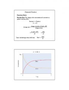
– Valid, feasible, and effective learning and teaching strategies about dynamic behavior using modeling and systems thinking in authentic practices can be realized (Spector 2000; Westra 2008). In the context of chemical kinetics, students are immediately confronted in a simulation of a reaction system with potential alternative conceptions. In the first example of cis-trans isomerization, a student can for instance observe in the graphs of the lower part of Fig. 1 that (i) it takes time before the equilibrium is reached; and (ii) at equilibrium, the concentrations of cis- and trans-complexes are not necessarily equal. More alternative conceptions about chemical equilibrium, which were listed in Subsection 2.1, can be addressed when one looks at rate-time and net rate-time graphs of the chemical equilibrium shown in Fig. 2.
where r1f = k1f ·[cis] , r1r = k1r ·[trans]. But the graphical model represents in fact more: it also represents an automatically generated computer program that solves this system numerically and allows the user to simulate the behavior of the modeled reaction system and to interpret the modeling results.
3.2 Strengths of Classical Graphical Modeling Tools Research indicates the following: – Despite the apparent difficulties of computer modeling in an inquiry approach, students can overcome the problems in a modeling task (Jacobson and Wilensky 2006; Sins 2006; Stratford et al 1998); – A graphical modeling tool supports novice modelers better in constructing their own models and in understanding other people’s models than modeling tools that require their users to work with textual representations in which they have to explicitly write down a sort of equation or a piece of programming code (L¨ohner 2005). – “Creating dynamic models has great potential for the use in classrooms to engage students in thought about science content, particularly in those thinking strategies best fostered by dynamic modeling: analysis, relational reasoning, synthesis, testing and debugging, and making explanations.” (Stratford et al 1998, p. 229) Through modeling, students can acquire model-based scientific reasoning skills (Milrad et al 2003) and learn about the specific domain (Ergazaki et al 2005; Schecker 1998); – Students can get more insight in the behavior of a dynamic system by running an executable model (Wilensky and Resnick 1999; Westra 2008);
Fig. 2 Rate-time and net rate-time graphs for cis-trans isomerization at 85 ◦ C.
Some of the points that a student could notice in the graphs displayed in Fig. 2 are: – The rate of the forward reaction decreases with time until equilibrium is reached (and not to completion); – The rate of the reverse reaction increases with time until equilibrium is reached; – The forward and reverse reaction rates are not always the same; – The forward and reverse reaction start at the same time;
7
– A system in equilibrium does not mean that the reactions ceased; – A system in equilibrium means that the net rate of concentrations is zero and that the forward- and reverse-reaction rates are equal.
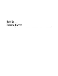
Executable models offer students the opportunity to observe the effects of changing the model or, less dramatically, of changing the parameter values and initial conditions. In fact, this has already been anticipated in the model shown in Fig. 1: The introduction of temperature T , the change of which has been simplified by the incorporation of a corresponding slider in the activity, is motivated by the wish to investigate the effect of temperature on the reaction system. Fig. 3 shows the results of a simulation of the isomerization at a lower temperature, namely at 80 ◦ C. The graphs of the previous simulation at a temperature of 85 ◦ C are shown in gray at the background to support easy comparison.
A student could discover from the graphs in Fig. 3 that changing the temperature – does not necessarily mean that the concentrations at equilibrium are affected. In other words, changing the temperature does not mean that the equilibrium constant is affected. – may change the magnitudes of the reaction rate constants without changing their ratio. In such case it only affects the time needed for the system to reach equilibrium; – may change the absolute magnitudes of the forward and reverse rates, also at equilibrium. It must be emphasized that these conclusions only hold because the isomerization is almost thermoneutral. It is actually a misconception to believe that the equilibrium constant is independent of temperature. When a chemical equilibrium is chosen in which activation energies of the forward and backward reactions differ substantially, a change in temperature will lead to a noticeable shift of the equilibrium. By changing the initial concentrations of the cisand trans-complex it can easily be verified that the system will always reach the same equilibrium concentrations, no matter what the starting concentrations are. By playing with the forward and reverse reaction rate constants, a student could discover that while the absolute magnitudes of the forward and reverse rate constants do not control the final equilibrium, equilibrium concentrations are controlled by the ratio of the rate constants.
3.3 Weaknesses of Classical Graphical Modeling Tools The graphical modeling of chemical kinetics illustrated by the example of cis-trans isomerization is rather simple. Other examples of reaction systems that can be dealt with in this way are unimolecular. Any other type of reaction system would lead for stoichiometric reasons to a disconnected, from chemical point of view incomprehensible graphical model. The basic example used in the paper to illustrate this is the gas-phase oxidation of nitric oxide: 2NO + O2 → 2NO2 . This example of a third-order rate reaction system has been chosen because it is a classical illustration of the fact that reaction rate data alone are not sufficient to determine the underlying reaction mechanism. The following three mechanisms have been identified by Tsukuhara et al (1999), which all lead to third-order reaction kinetics:
Fig. 3 concentration-time, rate-time, and net rate-time graphs for cis-trans isomerization at 80 ◦ C.
– A termolecular reaction, i.e., two molecules of NO and one O2 collide and form a transient complex, which in a single step forms two molecules of NO2 ;
8
– A pre-equilibrium mechanism with dimer of NO as an intermediate; – A pre-equilibrium mechanism with NO3 as an intermediate. The graphical model in Fig. 4 represents the termolecular reaction mechanism through the following coupled differential equations for the rate of change in the concentrations of the three species involved: d[NO] d [O2 ] d [NO2 ] = −2r, = −r, = 2r , dt dt dt
(3)
2
where r = k · [NO] · [O2 ] and the rate constant is given by the Arrhenius-type equation k = 1.2×103 ×10230/T . It also gives information about the units used.
of flow balance’), does not lead to the correct coupled differential equations. In other words, if both an arrow from [NO] toward [NO2] and an arrow from [O2] toward [NO2] were drawn, this would mean that the increase in concentration of NO2 over time is equal to the sum of the decrease in concentration of NO over time and the decrease in concentration of O2 over time. This is from chemical point of view incorrect for the given reaction. Moreover, the implication that both flows can be independently regulated is not true in chemical kinetics. In fact, due to the selected graphical modeling approach of level-flow diagrams, which is based on a metaphor of water tanks and valves, the diagrams for bi- and termolecular chemical reactions are inevitably disconnected. Forrester, the founder of the system dynamics and level-flow modeling approach in the context of socio-economic systems, was aware of this limitation and wrote (Forrester 1961, p. 70): “It should be noted that flow rates transport the content of one level to another. Therefore, the levels within one network must all have the same kind of content. Inflows and outflows connecting to a level must transport the same kind of items that are stored in the level. Items of one type must not flow into levels that store another type. For example, the network of materials deals only with material and accounts for the transport of the material from one inventory to another. Items of one type must not flow into levels that store another type.”
Fig. 4 Screen shot of the graphical model and simulation of the k
termolecular reaction 2NO + O2 − → 2NO2 .
Although the flow arrows, which represent the rate of change of concentrations, have been drawn in the graphical model such that the reader is given the impression of a chemical reaction in the form of a chemical network or a metabolic network, all of a sudden the icons that represent concentrations have become disconnected. The reason that one cannot directly draw physical flow arrows from reactants toward products is that the meaning of the graphical modeling tool, which is based on the level-flow model in which the sum of inflows in a level variable is by definition equal to the sum of outflows of this level variable (the so-called ‘principle
Clearly, chemical reactions do not meet this ‘principle of material consistency’ in the structure of a graphical model that is written in terms of levels interconnected by rates of flow: In a bimolecular reaction, two molecules may react to result in one molecule, that’s chemistry! On the other hand, it must be stressed that the problem only lies in the translation of the graphical model into the coupled differential equations that describe the kinetics of the chemical reaction. The fact that the conventions of a classical graphical system dynamics modeling tool, which state how the coupled differential equations or difference equations are to be generated from the graphical representation, are inconvenient for chemical kinetics comes even more to the fore when complex chemical reaction networks are modeled instead of elementary reactions. The following example, which is the simplest (‘MichaelisMenten’ and ‘Briggs-Haldane’) mechanism for a twostep enzyme-catalyzed reaction, will illustrate this: k
1f k )* − ES −−2f →E+P E+S−
k1r
9
where E, S, ES, and P are the unbound enzyme, substrate, intermediate enzyme-substrate, and product, respectively. One of the things students learn from or need to accept in this mechanism is that a species can simultaneously be involved in more than one reaction: the intermediate enzyme-substrate can both form a product as well as the original substrate. All reaction steps are considered as elementary reactions. See (Bruist 1998) and (Halkides and Herman 2007) for simulations of the reaction system with a spreadsheet, and (Mulquiney and Kuchel 2003) for simulations with a computer algebra system. A steady-state approximation is used in most cases to simplify the algebraic and computational work. The graphical model that represents this enzymecatalyzed reaction without using this approximation is shown in Fig. 5.
concentrations of the four species involved and it also gives the reader information about the units used for concentration and rate of change of concentration: d[S] = −r1f + r1r , dt d[ES] = r1f − r1r − r2f , dt
d [E] = −r1f + r1r + r2f , dt d[P] = r2f , (4) dt
where r1f = k1f ·[E]·[S] , r1r = k1r ·[ES] , r2f = k2f ·[ES]. Values of kinetic parameters have been taken from (Halkides and Herman 2007), which presents in fact a toy model of enzyme kinetics. Its unrealistic character is taken for granted because the graphical model of the reaction mechanism can still be used to convince students that the steady-state approximation makes sense. For example, using the computed time course of the enzyme-catalyzed reaction one can apply the regression tool in Coach 6 to find values of the Michaelis-Menten constant Km and of the maximum velocity Vmax by nonlinear regression and one can verify that these values are close to the theoretical values Km = (k1r + k2f )/k1f and Vmax = k1f · [E]|t=0 . Values of kinetic parameters found by nonlinear regression can also be compared with values obtained from a Lineweaver-Burk plot. Furthermore, the simulation tool can be used to discuss the validity of the steady-state approximation in the kinetic model. This example makes clear that a standard, rather simple chemical reaction network already leads to a disconnected graphical model in which the chemical reaction mechanism is obscured by the spaghetti (and meatballs) tangle of arrows and boxes. When the reaction mechanism of the enzyme-catalyzed reaction becomes more complicated, the corresponding graphical model that represents the chemical kinetics readily gets snarled up, to put it mildly. This happens, for example, when the urea cycle (Mulquiney and Kuchel 2003) is studied, a reaction network in which more than one substrate is available for the enzyme, more than one product is formed, and more than one enzyme may be involved. In summary, the following weaknesses have been identified and exemplified in using the classical graphical system dynamics modeling and simulation approach to chemical kinetics:
Fig. 5 Screen shot of the graphical model and simulation of the k1f
k
2f E + S −* )− ES −− → E + P reaction system.
k1r
The graphical model represents the following coupled differential equations for the rate of change in the
• Except for simple unimolecular reaction systems, the graphical models based on the traditional levelflow metaphor do not present a clear overview of the chemical reaction mechanism, but instead they have often an incomprehensible spaghetti (and meatballs) tangle of arrows and boxes. Especially the number of information arrows can be overwhelming.
10
• In most graphical models of chemical reaction systems levels represent concentrations of chemical species and flows represent rates of change of the species. Because the principle of flow balance holds in the level-flow metaphor, this means that graphical models of chemical reactions must be predominantly models in which levels are disconnected. Such a graphical model does not give any indication anymore of which species are reactants and which species are products of chemical reactions or reaction steps. The reaction mechanism is not clearly revealed in the graphical model. • Although many graphical modeling tools offer user interface elements such as knobs and sliders to set parameter values and initial conditions, not all of them allow their users to change values during a simulation run. Thus, many modeling tools do not offer much to investigate external effects on the kinetics of a chemical reaction system such as addition of extra reactants, depletion of products, and so on, in an exploratory approach. These difficulties in graphical modeling of chemical kinetics with level-flow based system dynamics modeling and simulation software are known and suggestions for improvement have been made. For example, the key ideas of chemical kinetics and thermodynamics have been expressed in a bond graph approach (Cellier 1991, ch. 9) and the level-flow metaphor has been replaced in (Elhamdi 2005; LeF`evre 2002, 2004) by the so-called kinetic process metaphor, which was inspired by graphical models of biochemical reaction networks and metabolic pathway systems. But these alternatives for and extensions of the traditional level-flow metaphor are at the level of system dynamics specialists and they are too complicated for use in chemistry education at high school level or first-year undergraduate level. In the next section, a much simpler graphical approach to modeling of chemical reactions is presented that covers the basics of chemical kinetics.
4 Improved Graphical Modeling of Chemical Reaction Systems A solution to most of the previously identified problems with classical graphical system dynamics modeling is presented in the form of an improved approach of chemical reactions based on a graph theoretic description of reaction kinetics. To this end, a new icon, viz. the Erlenmeyer flask symbol, is added to the graphical modeling tool. After a formal underpinning of the proposed extension, examples will illustrate the new approach to chemical kinetics. In Section 5, other applications of the
Erlenmeyer icon will be presented and this motivates the more general reference to this icon as a ‘process’ instead of a more chemistry related name like ‘reaction.’ In Subsection 4.3, the usefulness of adding interactivity elements such as sliders, buttons, and event controls to the graphical model tool will be illustrated.
4.1 Adding a Process Element to the Modeling Tool The improved graphical modeling approach of chemical reactions is based on a graph theoretic description of reaction kinetics that is similar to the oriented species-reaction graph introduced in (Craciun and Feinberg 2006) and the directed bipartite graph of a reaction network developed by Vol’pert and Ivanova (1987) [ see also (Vol’pert and Hudjaev 1985, ch. 12) ], more thoroughly analyzed in (Ermakov and Goldstein 2002; Mincheva and Roussel 2007), and for example implemented in a computer simulation and visualization environment for metabolic engineering (Qeli 2007). The graphical approach will be exemplified by the termolecular gas-phase oxidation of nitric oxide, which was also k discussed in Subsection 3.3, 2NO + O2 − → 2NO2 , with the associated system of differential equations: d[NO] d [O2 ] d [NO2 ] = −2r, = −r, = 2r , dt dt dt where for a given reaction rate constant k holds 2
r = k · [NO] · [O2 ] .
(5)
(6)
For a thorough description of the improved graphical approach it is wise to linger over chemical notation of reactions and reaction networks and its meaning. A chemical reaction network is formally defined (Feinberg 1979) as a triple (S, C, R) that consists of a finite set of chemical species (reactants and products of the reaction steps) S, a finite set of complexes (the objects before and after the reaction arrows) C, and a set of reactions R ⊂ C × C with the properties that (y, y) ∈ / R for any y ∈ C and that for each y ∈ C there exists a y 0 ∈ C such that (y, y 0 ) ∈ R or such that (y 0 , y) ∈ R. In plain words this means that each species must appear on the left- or right-hand side of at least one reaction step, that there are no superfluous species, that no complex reacts to itself, and that no complex is isolated. Henceforth the more suggestive y → y 0 is used in place of (y, y 0 ) when (y, y 0 ) ∈ R and equilibrium reactions are considered as two separate irreversible reaction steps. k In case of the reaction 2NO + O2 − → 2NO2 the sets are equal to S = {NO, O2 , NO2 }, C = {2NO + O2 , 2NO2 }, k
and R = {2NO + O2 − → 2NO2 }}. The stoichiometric coefficient of a species s in a complex y is the positive
11
integer in front of the species if it is contained in the complex and it is equal to zero otherwise. For example, in the complex 2NO + O2 the stoichiometric coefficients of NO, O2 , and NO2 are 2, 1, and 2, respectively. The kinetic graph of the chemical reaction network (S, C, R) is a directed graph in which the set of vertices is partitioned into two sets, namely, a set of species nodes and a set of reaction nodes. There is one species node for each species in the network and one reaction node for each (irreversible) reaction in the network. Each directed edge of the kinetic graph joins a species node to a reaction node or a reaction node to a species node (so the kinetic graph is a directed bipartite graph) according to the following prescription: Consider some reaction y → y 0 in R. There is one directed edge toward the reaction node y → y 0 coming from each node of a species present in the complex y of the reaction. There is one directed edge from the reaction y → y 0 toward each node of a species present in the complex y 0 . Otherwise stated, arrows are drawn for each reaction in the network from the reactants toward the reaction node and from the reaction node toward the products created in the reaction. The kinetic graph of the reaction k 2NO + O2 − → 2NO2 is shown in Fig. 6.
k
Fig. 6 The kinetic graph of the reaction 2NO + O2 − → 2NO2 .
Here, a species node is represented by a square and a reaction node is suggestively represented by an Erlenmeyer flask symbol. The directed bipartite graph is called a kinetic graph because it also incorporates by definition information about the kinetics of the chemical reaction. This information is about (contributions to) rates of change of species involved in the given reaction, based on the stoichiometric coefficients associated with the reaction: In this particular example, Formula (6) holds. In general, the elementary j th reaction in a reaction network kj
αj1 R1 + · · · + αjm Rm −→ βj1 P1 + · · · + βjn Pn has a reaction rate rj = kj · [R1 ]αj1 · · · · · [Rm ]αjm ,
(7)
where kj is the kinetic coefficient and P [Ri ] is the concentration of reactant Rj . Normally m αjm , which is the number of reactants involved in the j th reaction step, is a natural number less than or equal to 3. The time
course of the concentrations depends on the reaction rates rj : For example, the dynamics of [Ri ] and [Pi ] in the above reaction depends on rate rj in the form d [Ri ] = −αji rj , dt
d [Pi ] = βji rj . dt
(8)
In the kinetic graph, there exists a directed edge from the species node Rk toward the j th reaction node if αjk > 0 and similarly a directed edge from the j th reaction node toward the species node Pk if βjk > 0. Note that this formalism does not exclude the situation that reactants and products involve the same species (for example, in auto-catalytic reactions). The kinetic graph of a chemical reaction network clearly suggests how the classical level-flow formalism of graphical system dynamics modeling tools could be extended to function well for chemical reaction networks: A graphical icon for a reaction, say an Erlenmeyer flask symbol, must be added to the formalism and then levels can represent concentrations of species involved in the reaction network, provided that flows are between level icons and Erlenmeyer symbols. Inflows of an Erlenmeyer symbol originate from reactants and outflows of an Erlenmeyer symbol point at products in the chemical reaction that is symbolized by the Erlenmeyer flask. The Erlenmeyer symbol also represents the dynamics of the levels connected with it via the stoichiometry of the reaction: The Erlenmeyer symbol is linked to a formula for the reaction rate, which depends on the kinetic coefficient, the concentrations of reactants and their stoichiometric coefficients, and the stoichiometric coefficients determine the formulas for the inflows and outflows of the Erlenmeyer symbol. The improved graphical modeling of chemical reaction, based on kinetic graphs, leads to much clearer visual representations of chemical reaction networks for the following reasons: • Levels, flows, and process elements give a visual overview of the reaction mechanism; • The stoichiometry of a reaction already determines the formulas for the inflows and outflows so that there is no need to use information arrows from the reaction node toward these flows. The examples in the next subsection will illustrate that the new graphical models resemble more the pictures that chemists already draw for ages to illustrate reaction mechanisms. This is also the reason that students do not need to be introduced the kinetic graphs in the same formal way as was done in this subsection to underpin the proposed approach; a more informal introduction suffices to work with it in a sensible way.
12
4.2 Some Illustrative Examples The improved graphical modeling approach has been implemented in Coach 6 and the first example in this subsection is the same as the last example discussed in Subsection 3.3, namely, the two-step enzyme-catalyzed k1f k reaction E + S − )* − ES −−2f → E + P. This offers the reader k1r
the opportunity to compare the graphical model presented in Subsection 3.3 (Fig. 5) with the model based on the improved formalism (Fig. 7). The reader can also compare the graphical model of enzyme kinetics in Fig. 7 with the equivalent graphical model in Fig. 8, taken from (Lee and Yang 2008), that has been implemented in Powersim (www.powersim.no), another classical graphical modeling tool, and that does not reflect anymore the underlying reaction mechanism.
ysis of arginine to ornithine and urea catalyzed by the hydrolytic enzyme arginase, which is only one step of the urea cycle: k
1f k E+A− )* − EA −−2f → EO + U,
k1r
k3f
EO − )* −E+O k3r
where A, U, and O denote arginine, urea, and ornithine, respectively. The graphical model represents the following coupled differential equations for the rate of change in the concentrations of the species involved: d[E] d[A] = −r1f + r1r , = −r1f + r1r − r3r + r3f , dt dt d[EA] d[EO] = r1f − r1r − r2f , = r2f − r3f + r3r , dt dt d[U] d[O] = r2f , = r3f − r3r , (9) dt dt where
Fig. 7 Screen shot from the improved graphical model of the k1f
k
2f → E + P network. E + S −* )− ES −−
k1r
r1f = k1f · [E] · [A] ,
r1r = k1r · [EA] ,
r2f = k2f · [EA] ,
r3f = k3f · [EO] ,
r3r = k3r · [E] · [O] .
Values of kinetic parameters can be taken from (Kuchel et al 1977). The graphical model, the construction of which is envisioned to be doable by upper secondary school chemistry students or first-year undergraduate chemistry students, is very informative about the reaction mechanism. Thus, chemical kinetics of more realistic reaction mechanisms is not expected to be beyond the level of students anymore.
k1f
k
2f Fig. 9 Screen shot of the graphical model of E + A −* )− EA −− →
k1r
k3f
EO + U, EO −* )− E + O network. k3r
k
1f k2f Fig. 8 A model of E + S −* )− ES −− → E + P in Powersim.
k1r
4.3 Interactivity in Chemical Kinetics Modeling Because one of the goals was to make graphical system dynamics modeling of chemical kinetics viable in cases of more complicated reaction mechanisms, a second example is shown in Fig. 9, which would not be as comprehensible in a classical system dynamics graphical approach. It is the following enzyme-catalyzed reaction mechanism, taken from (Kuchel et al 1977; Maher et al 2003; Mulquiney and Kuchel 2003), for the hydrol-
Le Chˆatelier’s Principle is often used in textbooks to explain how a system in equilibrium responds to an external perturbation such as addition of a reactant, depletion of a product, change in pressure or temperature, and so on. Many research studies (Canpolat et al 2006; Cheung et al 2009; Qu´ılez 2004a; Qu´ılez-Pardo and Solaz-Portol´es 1995; Tyson et al 1999; Voska and
13
Heikkinen 2000) reported that teachers and students have difficulties in applying this principle appropriately and accurately. A common mistake is to reason that increasing the concentration of one of the reactants will result in an increase of the forward rate and a decrease of the reverse rate, because the forward reaction is favored over the reverse one. Such misinterpretations and misapplications of Le Chˆatelier’s Principle have brought Cheung et al (2009) and others (Allsop and George 1984; Qu´ılez 2004a) to question the appropriateness of this principle in chemistry education for predicting the direction in which a chemical equilibrium will shift when it is disturbed. In a qualitative or semi-quantitative approach to chemical equilibrium phenomena there is hardly any other instructional strategy than applying Le Chˆatelier’s Principle or reasoning with the Equilibrium Law. But then one better resists the temptation to combine this thermodynamic approach to chemical equilibrium, which does not make statements about forward or backward reactions, with a kinetic approach to chemical equilibrium based on the ‘law of mass action.’ A quantitative approach seems more suitable for discussing how chemical equilibrium is reached or how it changes when conditions change. This holds especially when a modeling and simulation environment offers tools to interactively change conditions during a simulation and/or allows an easy implementation of event-handling such as response to a sudden change in concentration, temperature, and so on. Furthermore, Solomonidou and Stavridou (2001) pointed at the potential of computer simulations and animations to help students construct appropriate conceptions about Le Chˆatelier’s Principle and the equilibrium constant law. Interactive change of initial conditions as well as event-handling of sudden changes during a simulation run have been implemented in the Coach 6 environment and are exemplified with the equilibrium shift of a gas mixture of hydrogen, iodine, and hydrogen as a response to a sudden change in hydrogen concentration and temperature. The reaction system under considerak1f )* − 2HI, where second-order rate kinetics tion is H2 +I2 − k1r
is assumed given by the following coupled differential equations for the rate of change in the concentrations of the three species involved: d [H2 ] = −r1f + r1r , dt d [HI] = r1f − r1r , dt
d [I2 ] = −r1f + r1r , dt (10) 2
where rf = kf · [H2 ] · [I2 ] , rr = kr · [HI] , and the Arrhenius equations for the rate constants are given (Graven 1956) for temperature T (in ◦ K) by kr =
7.18×10¹² ×e−24775/T and kf = 1.23×10¹² ×e−20646/T . It follows from these equations that the forward gas phase reaction is exothermic. Figure 10 is a screenshot of a simulation run based on this kinetic model.
k1f
*−2HI Fig. 10 Screen shot of the graphical model of the H2 +I2−) k1r
equilibrium reaction and a simulation with user interaction and an event during execution of the model.
Figure 10 shows a simulation run starting with only a nonzero concentration of HI at a temperature T = 721◦ K. After 6000 seconds the concentration of H2 is suddenly raised by 0.002 M, which has an immediate effect on the concentration time course. This sudden change is realized in the graphical model by introduction of an event (iconized by the thunderbolt symbol). The code behind this event icon is very simple: Once t>6000 then [H2] := [H2] + 0.002. The effect is that the equilibrium which was almost established is shifted right to less dissociation of hydrogen iodine. After a new equilibrium has been established established equilibrium, the user has pressed about 12000 seconds after the start of the reaction the button in the control panel to cause a sudden raise in temperature of 50◦ K. The effect is that the equilibrium shifts to the left, that is, more hydrogen iodide dissociates again. This is in agreement with the Le Chˆatelier Principle that states that increasing the temperature will shift the equilibrium to the left because the forward reaction is exothermic. Although the kinetic and thermodynamic approaches to chemical equilibrium phenomena are of different nature, results obtained by either method complement each other.
14
5 Other Applications Graphical modeling and simulation tools have other applications in chemistry education, for example in modeling and simulating acid-base titration curves (Heck et al 2010), and in other science fields [see for example (van den Berg et al 2008)]. Although no attention has been paid to it in this article so far, it is worth mentioning that the improved graphical modeling approach also has applications beyond chemical kinetics. This aspect is important in education because it would most probably not be worth the effort to add new elements to a general purpose graphical modeling tool if they were only relevant for a small part of the science curriculum. Students and teachers have to use their time effectively and economically. Much is won when students and teachers can use one and the same modeling environment for many science subjects. Then they have ample opportunities to grow into their roles of knowledgeable and skilled modelers of natural phenomena. We discuss two examples of usage of the new graphical formalism that are conceptually rather close to the chemical context of this paper. But one must realize that examples of completely different nature, such as for instance the modeling of the height of beer foam (Heck 2010), could be presented as well. The first example illustrates that quantitative pharmacokinetic models can be conveniently treated through the new graphical formalism. Fig. 11 shows a graphical model and simulation of the pharmacokinetics of the metabolism of ecstasy in the human body [taken from high school lesson materials “Swilling, Shooting, and Swallowing,” see also (Heck 2007)]: The improved graphical modeling approach provides a connected diagram that indicates the flow of the pharmacon in the body over time. The second example is the classical SIR (susceptibleinfected-recovered) epidemic model, also known as the Kermack and McKendrick (1927) model: S 0 = −βIS,
I 0 = βIS − αI,
R0 = αI .
(11)
The origin of the above system of differential equations can be a description of an epidemic though a compartmental model. Alternatively, the SIR model can be considered, like a chemical reaction network, as a two-step process with the following mechanism: β
S+I− → 2I,
α
I− →R
The first step in the process is linked with contact between healthy and infected persons, which leads to two infected persons. When an infected person has on average β contacts per day and infected persons are on
Fig. 11 Screen shot of a graphical model of pharmacokinetics of ecstasy in the human body and a simulation run with real data in the background.
average 1/α days ill, then the above system of differential equations follows from probabilistic considerations. Fig. 12 shows a graphical model based on a process network (the non-default stoichiometric coefficient has been added in the graphical model as an annotation).
Fig. 12 Screen shot of a process network based graphical model of the Kermack-McKendrick model of epidemics.
6 Conclusion A central aspect of inquiry learning is that the learners must develop their own models and in particular their own executable computer models of real world phenomena. Classroom experience and case studies indicate that this is possible at secondary school level when graphical system dynamics based software is used. Subsections 3.1 and 3.2 showed the potentiality of graphical system dynamics based modeling environments like STELLA in the context of chemical equilibrium and chemical kinetics. However, as was illustrated in Subsection 3.3, level-flow based modeling tools are of limited use in studying chemical kinetics when bi- or trimolecular reactions or chemical reaction networks come into play. It is tempting to associate in these graphical
15
models levels with concentrations of species in a reaction and physical flows with chemical reaction arrows, representing at the same time the kinetics of the reactions. But stoichiometry and plurimolecular reaction types are a spoil-sport. The graphical representation of a chemical reaction network in the form of a kinetic graph, as it has been introduced in Subsection 4.1, is more suitable. Only one thing is needed for this in the graphical level-flow formalism, namely, inclusion of a new icon for a reaction step. Then, levels can indeed represent concentrations of species and flows can represent changes in concentrations of species provided that these flows are between levels and reaction icons (the Erlenmeyer flask symbols in this paper). Each reaction icon is linked with a formula that describes the reaction rate and the stoichiometry of the reaction determines the formulas for the inflows and outflows of the reaction icon. In this way the graphical model gives a clear overview of the reaction mechanism (as was exemplified in Subsection 4.2). Another improvement comes from the addition of user interaction tools like sliders and button to influence simulation run while they are going on and of a special icon for discrete time event handling. This offers students the opportunity to explore “what if?” questions. An example of such an investigation of the influence of external effects on a chemical equilibrium was given in Subsection 4.3. Both improvements have been exemplified in this paper by the computer implementation in Coach 6. Furthermore, the examples in Sections 3 and 4 illustrated that alternative conceptions of students about chemical equilibrium and chemical kinetics, which were reviewed in Section 2, can be directly addressed with the (extended) graphical modeling approach. Section 5 contained some examples to briefly illustrate that this improved approach has applications beyond chemical kinetics and helps to clarify the dynamics of all kinds of real world phenomena. Acknowledgements The author would like to thank his colleagues Leendert van Gastel and Wolter Kaper for the fruitful discussions on the improved graphical modeling approach and their suggestions. Special thanks go to his colleague Martin Beugel for implementing and beta testing the new approach in the Coach 6 computer learning environment.
References Alberty RA (2004) Principles of detailed balance in kinetics. J Chem Educ 81(8):1206–1209 Allendoerfer RD (2003) KinSimXP, a chemical kinetics simulation. J Chem Educ 80(1):110 Allsop RT, George NH (1984) Le Chˆ atelier - a redudant principle? Educ in Chem 21(2):54–56
Banerjee AC (1991) Misconceptions of students and teachers in chemical equilibrium. Int J Sci Educ 13(4):487–494 Bengali AA, Mooney KE (2003) Synthesis, kinetics, and thermodynamics: an advanced laboratory investigation of the cis-trans isomerization of Mo(CO)4 (PR3 )2 . J Chem Educ 80(9):1044–1047 van den Berg E, Ellermeijer T, Slooten O (eds) (2008) Modeling in Physics and Physics Education. Proceedings of the GIREP Conference 2006, Amsterdam, The Netherlands, Amsterdam: Universiteit van Amsterdam Bergquist W, Heikkinen H (1990) Student ideas regarding chemical equilibrium. J Chem Educ 67(12):1000–1003 Bilgin I (2006) Promoting pre-service elementary students’ understanding of chemical understanding of chemical equilibrium through discussions in small groups. Int J Sci Math Educ 4(3):467–484 Blickensderfer R (1990) Learning chemical kinetics with spreadsheets. J Comput Math Sci Teach 9(4):35–43 Bruist MF (1998) Use of a spreadsheet to simulate enzyme kinetics. J Chem Educ 75(3):372–375 Canpolat N, Pınarba¸sı T, Bayrak¸ceken S, Geban O (2006) The conceptual change approach to teaching chemical equilibrium. Res Sci Tech Educ 24(2):217–235 Cellier FE (1991) Continuous System Modeling. Springer, New York, URL www.inf.ethz.ch/personal/fcellier/Pubs/BG/ springer chap9.pdf Chairam S, Somsook E, Coll RK (2009) Enhancing Thai students’ learning of chemical kinetics. Res Sci Techn Educ 27(1):95– 115 Cheung D, Ma HJ, Yang J (2009) Teachers’ misconceptions about the effects of addition of more reactants or products on chemical equilibrium Choi MMF, Wong PS (2004) Using a datalogger to determine first-order kinetics and calcium carbonate in eggshells. J Chem Educ 81(6):859–861 Chonacki N (2004) Stella: growing upward, downward, and outward. Comput Sci & Engin 6(3):8–15, DOI 10.1109/MCSE.2004.79 Cort´ es-Figueroa JE, Moore DA (1999) Using CBL technology and a graphing calculator to teach the kinetics of consecutive first-order reactions. J Chem Educ 76(5):635–638 Cort´ es-Figueroa JE, Moore DA (2002) Using a graphical calculator to determine a first-order rate constant when the infinity reading is unknown. J Chem Educ 79(12):1462–1464 Craciun G, Feinberg M (2006) Multiple equilibria in complex chemical reaction networks: II. The species-reaction graph. SIAM J Appl Math 66(4):1321–1338, DOI 10.1137/050634177 van Driel JH (2002) Students’ corpuscular conceptions in the context of chemical equilibrium and chemical kinetics. Chem Educ Res Pract Eur 3(2):201–213 van Driel JH, Gr¨ aber W (2002) The teaching and learning of chemical equilibrium. In: Gilbert JK, de Jong O, Justi R, Treagust DF, van Driel JH (eds) Chemical Education: Towards Research-based Practice, Kluwer Academic Publishers, Dordrecht, pp 271–292 van Driel JH, de Vos W, Verloop N, Dekker H (1998) Developing secondary students’ conceptions of chemical reactions: the introduction of chemical equilibrium. Int J Sci Educ 20(4):379– 392 van Driel JH, de Vos W, Verloop N (1999) Introducing dynamic equilibrium as an explanatory model. J Chem Educ 76(4):559–561 Elhamdi M (2005) Mod´ elisation et simulation de chaˆınes de valeurs en entreprise – Une approche dynamique des syst` emes ´ et aide ` a la d´ ecision: SimulValor. Phd thesis, L’Ecole Centrale
16 Paris, France, URL www.lgi.ecp.fr/∼yannou/Theses/These M Elhamdi 2005 - LCGI ECP.pdf Ergazaki M, Komis V, Zogza V (2005) High-school students’ reasoning while constructing plant growth models in a computer-supported educational environment. Int J Sci Educ 27(8):909–933 Ermakov GL, Goldstein BN (2002) Simplest kinetic schemes for biochemical oscillators. Biochem (Moscow) 67(4):473–484 Feinberg M (1979) Lectures on Chemical Reaction Networks. Lectures notes, 1979. URL www.che.eng.ohiostate.edu/∼FEINBERG/LecturesOnReactionNetworks Fermann J, Stamm K, Maillet A, Nelson C, SJ C, Spaziani M, Ramirez M, Vining W (2000) Discovery learning using Chemland simulation software. Chem Educat 5(1):31–37, DOI 10.1007/s00897000356a Ferreira MMC, Ferreira Jr W, Lino ACS, Porto MEG (1999) Uncovering oscillations, complexity, and chaos in chemical kinetics using Mathematica. J Chem Educ 76(6):861–866 Forrester J (1961) Industrial Dynamics, Students’ Edition. MIT Press, Cambridge MA, 7th printing Ganares K, Dumon A, Larcher C (2008) Conceptual integration of chemical equilibrium by prospective physical sciences teachers. Chem Educ Res Pract 9(3):240–249 Garnett PJ, Garnett PJ, Hackling MW (1995) Students’ alternative conceptions in chemistry: A review of research and implications for teaching and learning. Stud Sci Educ 25(1):69–95 Gorodetsky M, Gussarsky E (1986) Misconceptions of chemical equilibrium. Eur J Sci Educ 8(4):427–441 Graven WM (1956) High temperature reaction kinetics of the system H2 − HI − I2 . J Am Chem Soc 78(14):3297–3300 Griffiths AK (1994) A critical analysis and synthesis of research on students’ chemistry misconceptions. In: Schmidt HJ (ed) Problem Solving and Misconceptions in Chemistry and Physics, ICASE, Hong Kong, pp 70–99 Hackling MW, Garnett PJ (1985) Misconceptions of chemical equilibrium. Eur J Sci Educ 7(2):205–214 Hackling MW, Garnett PJ (1986) Chemical equilibrium: Learning difficulties and teaching strategies. Austral Sci Teach J 31(4):8–13 Halkides CJ, Herman R (2007) Introducing Michaelis-Menten kinetics through simulation. J Chem Educ 84(3):434–437 Halpern AM (2006) Computational studies of chemical reactions: the HNC − HCN and CH3 NC − CH3 CN isomerizations. J Chem Educ 83(1):69–75 Hameed H, Hackling MW, Garnett PJ (1993) Facilitating conceptual change in chemical equilibrium using a CAI strategy. Int J Sci Educ 15(2):221–230 Harvey E, Sweeney R (1999) Modeling stratospheric ozone kinetics. J Chem Educ 76(9):1309–1310 Heck A (2007) Modelling intake and clearance of alcohol in humans. Electron J Math Technol 1(3):232–244, URL https://php.radford.edu/∼ejmt Heck A (2010) Bringing reality into the classroom. Teach Math Appl (in press) Heck A, Kedzierska E, Ellermeijer T (2009) Design and imple, mentation of an integrated computer working environment for doing mathematics and science. J Comput Math Sci Teach 28(2):147–161 Heck A, Kedzierska E, Rogers L, Chmurska M (2010) , Acid-base titration curves in an integrated computer learning environment, URL www.science.uva.nl/∼heck/ research/art/AcidBaseTitration.pdf, in press Huddle PE, Pillay AE (1996) An in-depth study of misconceptions on stoichiometry and chemical equilibrium at a south african university. J Res Sci Teach 33(1):65–77
Huddle PE, White MW (2000) Simulations for teaching chemical equilibrium. J Chem Educ 77(7):920–926 Jacobson MJ, Wilensky U (2006) Complex systems in education: Scientific and educations importance and implications for the learning sciences. J Learn Sci 15(1):11–34 Justi R (2002) Teaching and learning chemical kinetics. In: Gilbert JK, de Jong O, Justi R, Treagust DF, van Driel JH (eds) Chemical Education: Towards Research-based Practice, Kluwer Academic Publishers, Dordrecht, pp 293–315 Kermack WO, McKendrick AG (1927) A contribution to the mathematical theory of epidemics. Proc R Soc Lond A 115:700–721 Kosinsky B (2001) Teaching reaction equilibrium using Stella modeling software. In: O’Donnel M (ed) Proceedings of the 23rd Workshop/Conference of the Association for Biology Laboratory Education, University of Chicago, USA, 2001, pp 155–274, URL www.ableweb.org/volumes/vol23/15-kosinski.pdf Kousathana M, Tsaparlis G (2002) Students’ error in solving numerical chemical-equilibrium problems. Chem Educ Res Pract Eur 3(1):5–17 Kuchel PW, Roberts DV, Nichol LW (1977) The simulation of the urea cycle: correlation of effects due to inborn errors in the catalytic properties of the enzymes with clinical-biochemical observations. Austral J Exp Biol Med Sci 55(3):309–326, DOI 10.1038/icb.1977.26, URL www.nature.com/icb/journal/v55/n3/pdf/icb197726a.pdf Lee JD, Briggs AG (1978) A computerized approach to simple chemical kinetics. Comput Educ 2(1/2):89–115 Lee WP, Yang KG (2008) Applying intelligent computing techniques to modeling biological networks from expression data. Geno Prot Bioinfo 6(2):111–120 LeF` evre J (2002) Kinetic process graphs: building intuitive and parsimonious material stock-flow diagrams with modified bond graph notations. In: Davidsen P, Mollona E, Diker V, Langer R, Rowe J (eds) Electronic Proceedings of the 20th International Conference of the System Dynamics Society, Palermo, Italy, 2002, URL http://systemdynamics.org/conferences/2002/papers/ Lefevre1.pdf LeF` evre J (2004) Why and how should we replace the tank-pipe analogy or our stock-flow models by a chemical process metaphor? In: Kennedy M, Winch G, Langer R, Rowe J, Yanni J (eds) Electronic Proceedings of the 22th International Conference of the System Dynamics Society, Oxford, England, 2004., URL http://systemdynamics.org/conferences/2004/SDS 2004/ PAPERS/379LEFEV.pdf de Levie R (2002) Spreadsheet simulation of chemical kinetics. Crit Rev Anal Chem 32(1):97–107 Locaylocay J, van den Berg E, Magno M (2005) Changes in college students’ conceptions of chemical equilibrium. In: Boersma K, Goedhart M, de Jong O, Eijckelhof H (eds) Research and the Quality of Science Education, Springer, Dordrecht, pp 459–470 L¨ ohner S (2005) Computer-based modeling tasks: The role of external representations. PhD thesis, Universiteit van Amsterdam Maher AD, Kuchel PW, Ortega F, de Atauri P, Centelles J, Cascante M (2003) Mathematical modelling of the urea cycle: a numerical investigation into substrate channelling. Eur J Biochem 270(19):3953–3961, DOI 10.1046/j.14321033.2003.03783.x Maia PF, Justi R (2009) Learning of chemical equilibrium through modelling-based teaching. Int J Sci Educ 31(5):603– 630
17 Miles Jr DG, Francis TA (2002) A survey of computer use in undergraduate physical chemistry. J Chem Educ 79(12):1477– 1479 Milrad M, Spector JM, Davidson PI (2003) Model facilitated learning. In: Naidu S (ed) Learning & teaching with technology: Principles and practices, Kogan Page, London, pp 13–28 Mincheva M, Roussel MR (2007) Graph-theoretic methods for the analysis of chemical and biochemical networks. I. multistability and oscillations in ordinary differential equation models. J Math Biol 55(1):61–86, DOI 10.1007/s00285-007-0099-1 Mira J, Gonz´ alez Fen´ andez C, Mart´ınez Urreaga J (2004) Two examples of deterministic versus stochastic modeling of chemical reactions. J Chem Educ 80(12):1488–1493 Mulquiney PJ, Kuchel PJ (2003) Modelling Metabolism with Mathematica. CRC Press LLC, New York Ogilvie JF, Monagan MB (2007) Teaching mathematics to chemistry students with symbolic computation. J Chem Educ 84(5):889–896 ¨ Ozmen H (2008) Determination of student’s alternative conceptions about chemical equilibrium. Chem Educ Res Pract 9(3):225–233 Pedrosa MA, Diaz MH (2000) Chemistry textbook approaches to chemical equilibrium and student alternative conceptions. Chem Educ Res Pract Eur 1(2):227–236 Piquette JS (2001) An analysis of strategies used by chemistry instructors to address students alternate conceptions in chemical equilibrium. PhD thesis, University of Northern Colorado, URL http://archiv.ub.unimarburg.de/diss/z2007/0108/pdf/deq.pdf Piquette JS, Heikkinen HW (2005) Strategies reported used by instructors to address student alternate conceptions in chemical equilibrium. J Res Sci Teach 42(10):1112–1134 Posner G, Strike K, Hewson P, Gertzog W (1982) Accomodation of a scientific conception: Toward a theory of conceptual change. Sci Educ 66(2):211–227 Qeli E (2007) Information visualization techniques for metabolic engineering. PhD thesis, Philipps-Universit¨ at, Marburg, Germany, URL http://archiv.ub.unimarburg.de/diss/z2007/0108/pdf/deq.pdf Qu´ılez J (2004a) Changes in concentration and in partial pressure in chemical equilibria: Students’ and teachers’ misunderstandings. Chem Educ Res Pract 5(3):281–300 Qu´ılez J (2004b) A historical approach to the development of chemical equilibrium through the evolution of the affinity concept: Some educational suggestions. Chem Educ Res Pract 5(1):69–87 Qu´ılez-Pardo J, Solaz-Portol´ es J (1995) Students’ and teachers’ misapplication of le chatelier’s principle: Implication for the teaching of chemical equilibrium. J Res Sci Teach 32(9):939– 957 Reid KL, Wheatley RJ, Brydges SW, Horton JC (2000) Using computer assisted learning to teach molecular reactions dynamics. J Chem Educ 77(3):407–409 Ricci RW, van Doren JM (1997) Using dynamic simulation software in the physical chemistry laboratory. J Chem Educ 74(11):1372–1374 Schecker HP (1998) Physik – Modellieren, Grafikorientierte Modelbildungssysteme im Physikunterricht. Klett Verlag, Stuttgart Seybold PG, Kier LB, Cheng CK (1997) Simulation of first-order chemical kinetics using cellular automata. J Chem Inf Comput Sci 37(2):386–391, DOI 10.1021/ci960103u Sins PHM (2006) Students’ reasoning during computer-based scientific modeling. Phd thesis, Universiteit van Amsterdam, The Netherlands, URL http://dare.uva.nl/document/22567
Solomonidou C, Stavridou H (2001) Design and development of a computer learning environment on the basis of students’ intial conceptions and learning difficulties about chemical equilibrium. Educ Inf Technol 6(q):5–27 Spector JM (2000) System dynamics and interactive learning environments: Lessons learned and implications for the future. Simul Gaming 31(4):528–935 Steffen LK, Holt PL (1993) Computer simulations of chemical kinetics. J Chem Educ 70(12):991–993 Stieff M, Wilensky U (2003) Connected chemistry - incorporating interactive simulations into the chemistry classroom. J Sci Educ Technol 12(3):285–302, DOI 10.1023/A:1025085023936 Stratford SJ, Krajcik J, Soloway E (1998) Secondary students’ dynamic modeling processes: Analyzing, reasoning about, synthesizing, and testing models of stream ecosystems. J Sci Educ Tech 7(3):215–234 Tsukuhara H, Ishida T, Mayumi M (1999) Gas-phase oxidation of nitric oxide: Chemical kinetics and rate constant. Nitric Oxide: Biol Chem 3(3):191–198 Tyson L, Treagust DF, Bucat RB (1999) The complexity of teaching and learning chemical equilibrium. J Chem Educ 76(4):554–558 Vol’pert A, Hudjaev S (1985) Analysis in Classes of Discontinuous Functions and Equations of Mathematical Physics. Martinus Nijhoff Publishers, Dordrecht Vol’pert A, Ivanova A (1987) Mathematical models in chemical kinetics. In: Mathematical Modeling of Nonlinear Differential Equations of Mathematical Physics, Work Collect., Nauka, Moscow, pp 57–102 Voska KW, Heikkinen HW (2000) Identification and analysis of student conceptions used to solve chemical equilibrium problems. J Res Sci Teach 37(2):160–176 Westra RHV (2008) Learning and teaching ecosystem behaviour in secondary education. Phd thesis, Universiteit Utrecht, The Netherlands, URL http://igitur-archive.library.uu.nl/dissertations/2008-0220200526/westra.pdf Wilensky U, Resnick M (1999) Thinking in levels: A dynamic systems apporach to making sense of the world. J Sci Educ Technol 8(1):3–19 Zielinski TJ (1995) Promoting higher-order thinking skills: uses of Mathcad and classical chemical kinetics to foster student development. J Chem Educ 72(7):631–637