FACULTEIT ECONOMIE EN BEDRIJFSKUNDE TWEEKERKENSTRAAT 2 B-9000 GENT Tel. Fax.
: 32 - (0)9 – 264.34.61 : 32 - (0)9 – 264.35.92
WORKING PAPER
Modeling complex longitudinal consumer behavior with Dynamic Bayesian Networks: An Acquisition Pattern Analysis application Anita Prinzie 1 Dirk Van den Poel 2
August 2009 2009/607
1
Corresponding author: Dr. Anita Prinzie, Senior Researcher Manchester Business School, Manchester, UK, Visiting Professor at Faculty of Economics and Business Administration, Ghent University:
[email protected]; PhD Candidate, Ghent University, more papers about customer relationship management can be obtained from the website: www.crm.UGent.be. 2 Prof. Dr Dirk Van den Poel, Professor of Marketing Modeling/analytical Customer Relationship Management, Faculty of Economics and Business Administration,
[email protected].
D/2009/7012/59
Modeling complex longitudinal consumer behavior with Dynamic Bayesian Networks: An Acquisition Pattern Analysis application Anita Prinzie Manchester Business School and Ghent University
[email protected] and
[email protected]
Dirk Van den Poel Ghent University
[email protected] Abstract Longitudinal consumer behavior has been modeled by sequence analysis. A popular application involves Acquisition Pattern Analysis exploiting typical acquisition patterns to predict a customer’s next purchase. Typically, the acquisition process is represented by an extensional, unidimensional sequence taking values from a symbolic alphabet. Given complex product structures, the extensional state representation rapidly evokes the state-space explosion problem. Consequently, most authors simplify the decision problem to the prediction of acquisitions for selected products or within product categories. This paper advocates the use of intensional state definitions representing the state by a set of variables thereby exploiting structure and allowing to model complex, possibly coupled sequential phenomena. The advantages of this intensional state space representation are demonstrated on a financial-services cross-sell application. A Dynamic Bayesian Network (DBN) models longitudinal customer behavior as represented by acquisition, product ownership and covariate variables. The DBN provides insight in the longitudinal interaction between a household’s portfolio maintenance behavior and acquisition behavior. Moreover, it exhibits adequate predictive performance to support the financial-services provider’s cross-sell strategy comparable to decision trees but superior to MulltiLayer Perceptron neural networks.
Keywords: state space representation, longitudinal, sequence analysis, acquisition pattern analysis, cross-sell, analytical Customer Relationship Management
2
1 Introduction Sequence analysis has become common place in the longitudinal analysis of consumer behavior. One of the most popular applications is Acquisition Pattern Analysis, describing the next logical product/service acquisition for a customer, based on the sequential pattern of a customer’s acquisition history and on the pattern of other customers. Extant research testifies to a common order in which household units acquire durable goods (Clarke and Soutar 1982; Corfman et al. 1991, Dickson et al. 1983; Feick 1987; Hauser and Urban 1986; Hebden and Pickering 1974; Lush et al. 1978; Kasulis et al. 1979; Mayo and Qualls 1987; Pyatt 1964; Paroush 1965; McFall 1969; Prinzie and Van den Poel 2007) or financial services (Dickenson and Kirzner 1986; Kamakura et al. 1991; Li et al. 2005; Paas 1998; Paas, Bijmolt and Vermunt 2007; Paas and Molenaar 2005; Paas, Vermunt and Bijmolt 2007; Prinzie and Van den Poel 2006; Stafford et al. 1982, Soutar and Ward 1997). Minor divergences from this common order of acquisition might stem from cultural differences just like a companies reputation varies between cultures (Falkenreck and Wagner 2008). Notwithstanding these slight deviations, marketing managers can exploit this common acquisition order; i.e. priority pattern, to support cross-selling efforts aimed to augment the number of products/services customers acquire from a firm. Typically, the customer’s longitudinal acquisition sequence is represented as an unstructured, unidimensional sequence, thereby limiting the practical value of any cross-sell model inferred from it in multiple ways. Firstly, the unidimensional representation impedes capturing the acquisition behavior at a sufficient level of detail or for the full product range. For example, in an lth-order Markov model the next acquisition is described by l previous values of one random variable Xt , taking values from a symbolic alphabet N={1, …, M}. This extensional representation of the customer’s acquisition state, one in which each state is explicitly named rather than described by variables as in an intensional state representation (Boutilier, Dean and Hanks 1999), rapidly results in an explosion of the state space and as a consequence computational intractability of the methods modelling this information. To illustrate this difference between an extensional and an intensional state representation, assume we want to represent a household’s longitudinal holiday behavior. An extensional state definition represents the household’s holiday sequence by literally mentioning the name of the consecutive holiday destinations: e.g., Puerto Plata Æ Paris Æ Tirol. This extensional state definition of holiday behavior literally lists all possible holiday destinations rapidly leading to a very long list and hence state space explosion. On the other hand, an intensional state definition will define a holiday by describing the properties of a holiday in multivalued features or state variables. For example the same longitudinal holiday behavior could be described by two state variables: activity {sun bath, ski, scuba dive, hiking, visiting attractions} and distance {short, medium, long}: (sun bath, long) Æ (visiting attractions, short) Æ (ski, medium). Describing the set of holiday destinations by state variables (intensional representation) is much sparser than listing all possible holiday destinations (extensional representation). Analogously, representing acquisition behavior by literally mentioning the acquired products as opposed to describing the features of the products acquired in state variables is often computational intractable. Therefore, in practice, the state-space explosion problem forces the researcher either to select a limited set of products or to analyze the acquisition behavior at less detailed level, e.g. product 3
categories. In both scenarios, the cross-sell predictive performance and practical value are limited. In the first scenario, the customer might acquire a product or service not included in the acquisition pattern analysis. In the last scenario, marketing communication at the product category level might lack specificity and consequently effectiveness. Secondly, the analysis of acquisition behavior as a unidimensional process largely neglects that the longitudinal acquisition behavior might be related to other longitudinal behavior like portfolio evolution and other covariates changing over time. Analogous to tree-based decision systems capturing multivariate crosssectional interactions (Yada, Ip and Katoh 2007), the Latent Markov analysis has been employed (Paas, Bijmolt and Vermunt 2007; Paas, Vermunt and Bijmolt 2007) to model the interaction between the longitudinal acquisition process and covariates changing over time. However, a latent Markov model is unable to model longitudinal interactions as opposed to a Dynamic Bayesian Network. A latent Markov model assumes that, when controlling for covariate values at time t, the latent class membership only depends on the previous class membership at time t-1. Hence, unlike Dynamic Bayesian Networks (DBNs), a latent Markov model does not allow modeling coupled processes; i.e. longitudinal interactions, like the simultaneous evolution of the acquisition sequence with the evolution of one or more covariates also exhibiting a Markov property. Thirdly, the adoption of an extensional rather than factored or intensional state space representation largely ignores the structure exhibited by the product/service space and typically results in a simplified representation of the decision environment. However, most marketing problems, including cross-sell problems, exhibit considerable structure (e.g. products can be structured according to their attributes or target groups, Baier and Gaul 1999; Kagie, van Wezel and Groenen 2008) and thus can be solved using special-purpose methods that recognize that structure (Boutilier, Dean and Hanks 1999). Amongst other techniques, Dynamic Bayesian Networks (DBNs) could be employed to exploit the structure of the state. DBNs generalize (hidden) Markov models by allowing states to have internal structure. DBNs represent the state of the environment (e.g. customer) by a set of variables; i.e. intensional state representation as opposed to (hidden) Markov’s extensional state representation. The DBN models the probabilistic dependencies of the variables within and between time steps. If the dependency structure is sufficiently sparse, it is possible to analyze real-life problems with much larger state spaces than using Markov models. In addition to reducing computational complexity while maintaining the decision problem’s complexity, DBN’s intensional state-space representation enables the marketing manager to gain insight into the structure of the problem, in case the customer’s acquisition process. This paper illustrates the advantages of Dynamic Bayesian Networks for acquisition pattern analysis with the aim to support the cross-sell strategy of a financial-services provider. The DBN models multidimensional customer behavior as represented by acquisition, product ownership and life-cycle sequences. The results convey that, in addition to the ability to model structured multidimensional, potentially coupled, sequences, the DBN exhibits adequate predictive performance to support the financial-services provider’s cross-sell strategy. The DBN outperforms MultiLayer Perceptron neural networks and it has comparable predictive performance to decision trees, while providing more insight in the longitudinal interactions.
4
The remainder of the paper is structured as follows. In the Methodology Section, we briefly present the Dynamic Bayesian Networks. In Section 3, we describe the cross-sell application demonstrating the advantage of DBNs for acquisition pattern analysis. Section 4 discusses the main findings. Finally, the last section draws conclusions and suggests avenues for further research.
2 Methodology 2.1 Dynamic Bayesian Networks as an extension of Bayesian Networks A Bayesian Network encodes the joint probability distribution of a set of variables, {Z1, …, Zd} as a directed acyclic graph expressing conditional dependencies and a set of conditional probability models. Each node corresponds to a variable which can be discrete or continuous. The model computes the probability of a state of the variable given the state of its parents. The set of parents of Zi, denoted by Pa(Zi), is the set of nodes with an arc to Zi in the graph. The structure of the network encodes that each node is conditionally independent of its nondescendants given its parents. The probability of an arbitrary event Z = (Z1, …, Zd) is computed as follows: P (Z ) = ∏ id=1 P (Z i Pa ( Z i ) )
(1)
Dynamic Bayesian Networks (DBNs) (Dean and Kanazawa 1989) extend Bayesian Networks for modeling dynamic systems thereby also exploiting conditional independence. In a DBN, a state at time t is represented by a set of random variables Zt = (Zi,t, …, Zd,t). The set of Zt could be divided into unobserved state variables Xt and observed state variables Yt which can be discrete or continuous. In a two-time slice Bayesian Network the state at time t+1, Zt+1 is only dependent on the immediately preceding state Zt, i.e. P(Zt+1|Zt) or first-order Markov property. Typically, the transition models are assumed to be invariant across time slices, i.e. a stationary process. A DBN is a pair of Bayesian networks (B0, BÆ) where B0 represents the initial distribution P(Z0) and BÆ is a two-time slice Bayesian Network (2TBN) defining the transition distribution. Studying these initial and transition distributions as embodied by the respective Conditional Probability Distributions (CPDs) enable the manager to gain insight into the within and between time-slice dependencies. The representation of the CPD defining a particular P(Zi|Pa(Zi)) depends on whether the child Zi is discrete or continuous and whether the parents are discrete, continuous or a mixture. Firstly, we discuss some of the possible types of CPD given the child Zi is discrete. If all its parents Pa(Zi) are discrete then the CPD is a multinomial distribution represented by a Conditional Probability Table (CPT). If all its parents Pa(Zi) are continuous then the CPT could be a multinomial logit function or a multi layer perceptron. If its parents Pa(Zi) are a mixture of discrete and continuous state variables then the CPD could be a mixture of multinomial logit functions or a mixture of multi layer perceptrons. Secondly, if the child Zi is continuous then the CPD could be a conditional linear Gaussian or a mixture of Gaussians. The joint distribution represented by a DBN; joining the initial distribution and the transition distributions, is obtained by unrolling the 2TBN as follows: 5
T
(
P ( Z 0 ,..., Z T ) = P ( Z 0 ) P ( Z 0 Pa ( Z 0 ) ∏ P ( Z t Z t − 1 ) P Z t Pa ( Z t )
)
(2)
t =1
2.2 Predictive Model Evaluation: class-specific PCCs and wPCC The predictive performance of the Dynamic Bayesian Network is evaluated in terms of class-specific Percentage Correctly Classified (PCCs) and the overall wPCC on a separate validation and test set, i.e. data sets of instances not used for model estimation. In absence of a specific predictive objective, e.g. predict classes k=1 and k=3 well, we evaluate the DBN in terms of its ability to correctly classify cases in all classes K. Given this objective and the class imbalance of the dependent, it is inappropriate (Barandela et al. 2003) to express the classification performance in terms of the average accuracy like the Percentage Correctly Classified (PCC). Analogous to Morrison’s (1969) proportional chance criterion, the predictive evaluation of the models should take the distribution of the multinomial dependent into consideration. Firstly, we will weigh the class-specific PCCs with regard to the prior class distribution. Each class k (k ∈ K) of the dependent has a strict positive weight wk (3), with fk referring to the relative frequency of the class on the dependent variable. The class-specific weights sum to one as in (3). Given the weights, the weighted PCC equates to (4):
wk =
1 − fk K
∑1 − f k
K
s.t.
∑ wk = 1
(3)
k =1
k =1
wPCC = ∑k =1 wPCCk K
(4)
with wPCC k = w k * PCC k . The weighted PCC is related to the balanced error rate. We penalize models predicting several alternatives by equally dividing the 100% classified over all alternatives predicted. Secondly, we benchmark the model’s performance to the proportional chance criterion Crpro rather than the maximum chance criterion Crmax (Morrison 1969):
Crpro =
K
∑ f k2
(5)
k =1
3 A Financial-Services Cross-sell Application The benefits of Dynamic Bayesian Networks (DBNs) for acquisition pattern analysis are illustrated in a financial-services cross-sell application. From a data warehouse of an international financial-services provider a household’s acquisition sequence is derived in eleven service categories (Table 1). Notice that 6
the acquisition sequences are constructed at the household level, as household units are the principal decision-making unit in the financial-services market (Guiso et al. 2002). The objective is to extract patterns from the acquisition sequences enabling to predict the next financial service acquisition for each household. Unlike most previous research in Acquisition Pattern Analysis, the longitudinal acquisition behavior is augmented with other longitudinal behavior like the household’s service portfolio sequence at each acquisition event. A household reducing the number of financial products between two acquisition events should have a smaller service portfolio at the second acquisition event. Furthermore, we address the effect of the household’s family life-cycle on the household’s service portfolio at a given acquisition moment. Table 2 defines the intensional state space representation. The ownership state variables clearly reflect the structure of financial services, which can be partitioned into investments, credits, checking accounts and insurances. The latter reflects how DBNs exploit structure intrinsic to the environment. The ownership state variables at time t incorporate the newly acquired service at time t, thereby revealing information on how the household’s financial portfolio has been enriched by the newly acquired service. The age state variable is a proxy for the household’s stage in the family-life cycle. Households residing in different stages of the family-life cycle typically hold different service portfolios due to household need evolution (Hebden and Pickering 1974; Kamakura et al. 1991; Mayo and Qualls 1987; Paas, Bijmolt and Vermunt, 2007). The operationalization of the family-life cycle is based on the Wells and Gubar’s (1966) Family Life-Cycle (FLC) model defining family life-cycle stages by age of the household head, employment status of the household head, and the age of the youngest child (see Table 3). As the employment status of the household head was not for all households known and the age of the youngest child was typically unknown, the family life-cycle is solely based on the age of the household head. From the FLC model three aggregated family life-cycle stages based on age can be derived (see last column in Table 3): 1) FLC group 1: 35 - : young couple, young parents 1 and young parents 2, 2) FLC group 2: age [35, 54[ : mature parents 1, mature parents 2, and mature couple and 3) FLC group 3: age 55 + : retired couple. By defining different Dynamic Bayesian Network architectures through specifying alternative within-time slice and between-slice effects for the state variables in Table 2 and selecting the best network architecture, the marketing manager gains insight in how the different longitudinal dimensions influence each other. How are the acquisition sequence, the portfolio sequence and the life-cycle sequence related? Section 3.2 discusses the various network architectures estimated and identifies the best network architecture. Beforehand the data and the data preparation are elaborated on in next Section 3.1. 3.1 Data and Data Preparation From the original database of the financial-services provider containing information on approximately 860,000 households, households are selected with at least two acquisition dates. The latter ensures the reliable estimation of the transition probabilities from one acquisition event to the next. Households with an exceptional high number of services acquired or with too many missing values on the service category are deleted. After data preparation, 600,340 households are retained. We randomly assigned 200,113 households to the estimation sample, 7
200,114 households to the validation sample and the remaining 200,113 households to a test sample. 3.2 Dynamic Bayesian Network Architecture Selection To infer how the longitudinal dimensions are related different Dynamic Bayesian Network architectures are defined by specifying different within-time slice and between-time slice effects between the state variables listed in Table 2. 3.2.1 Within-Time Slice Effects All DBNs provide in a within-time slice effect of age on a household’s service portfolio in accordance to the life-cycle hypothesis. The alternative DBNs differ as to which within-time slice effects are determined between the ownership state variables reflecting the structured financial-services product space. To guide the definition of different within-time slice effects between the ownership state variables, we estimated Kendall’s tau association between the ownership state variables. All association measures in Table 4 are statistically significant at α=0.001 thereby providing further insight into the structure in the financial-services product space. Table 4 portrays a large negative association between the household’s ownership of investment products and insurances. The second largest association exists between the ownership of credits and checking accounts. Finally, the third largest association exists between the ownership of investment products and checking accounts. The next association is smaller than 0.20 in absolute value and is not considered for constructing the alternative DBNs. 3.2.2 Between-Time Slice Effects Each DBN specifies between-time slice effects of service portfolio and service acquisition on the household’s next service acquisition. The alternative DBNs differ in whether they include a first-order Markov effect between service portfolio (from now on referred to as Markov Portfolio) or not (from now on referred to as No Markov Portfolio). Allowing for this Markov property on a covariate like service portfolio would be impossible within a Latent Markov model. 3.2.3 DBN Network Selection Consecutively we estimate for each between-time slice network architecture (i.e. No Markov Portfolio and Markov Portfolio) (a) a DBN without within-time slice effect between the ownership state variables (Table 5), (b) two DBNs based on the strongest association between the investment and insurance ownership state variables (Table 6), (c) all possible DBNs based on the two strongest associations between the ownership state variables (Table 7), and (d) all possible DBNs based on the three strongest associations (Table 8). In total 30 (2*15) alternative DBN models have been estimated on a random sample of 50,000 households drawn from the estimation sample (200,113 households). Table 5 to Table 8 report the model fit of the various DBNs. LL refers to the log likelihood where log denotes the natural logarithm. The Bayesian Information Criterion (BIC) balances the desire for a better fitting model against the desire for a parsimonious model: 8
BIC = −2 LL + p log(n)
(6) where LL is the log likelihood, p is the number of independent parameters and n is the number of components in the log-likelihood (Schwarz, 1978). The Consistent Akaike’s Information Criterion (CAIC) was defined by Bozdogan (1987) as a consistent version of the AIC statistic thereby resolving the latter’s magic number ‘2’ problem:
CAIC = −2 LL + p(log(n ) + 1)
(7)
The DBN with the smallest CAIC is selected as final network architecture. Given the large data set at hand the CAIC criterion is preferred to AIC2 and AIC3 as CAIC’s general tendency to underfit reduces with sample size, whereas AIC2 and AIC3 tend to overfit with increasing sample size (Bozdogan 1987). Inspecting the CAIC statistics in Tables 5 to 8 clearly reveals that a DBN incorporating a first-order effect on the household’s service portfolio (Markov Portfolio models) largely outperforms an identical DBN except for the absence of such a Markov effect (No Markov Portfolio). The latter shows the advantage of DBNs to latent Markov models in allowing the researcher to assess the need for a Markov effect for the covariates. The best DBN with the lowest CAIC appears in bold in Table 8. Figure 1 shows the final Dynamic Bayesian Network architecture modeling 1) the within-time slice effect of checking account ownership on the ownership of credits, 2) the within-time slice effect of investment ownership on the ownership of checking accounts, 3) the within-time slice effect of investment ownership on the ownership of insurances, 4) the within-time slice effect of a household’s family life cycle (age) on a household’s portfolio, 5) the betweentime slice effects of service portfolio and service acquisition on the household’s next service acquisition, and 6) the between-time slice effects of service portfolio on the household’s next service portfolio 3 .
4 Results 4.1 Predictive Performance of Selected DBN Model We estimated the selected DBN illustrated in Figure 1 using the full-length acquisition sequences of the 200,113 households in the estimation sample. The selected DBN was estimated with the parameters of the selected DBN on the small estimation sample (50,000 households) as starting values. The predictive performance of the DBN indicates how well it is able to predict for all households in a specific sample the 2-nd until last acquisition event. The robustness of the predictive performance of the selected DBN is assessed by applying the DBN on the large validation (200,114 households) and large test sample (200,113 households). Table 9 reports the predictive performance on the estimation, validation and test samples with respect to the wPCC and the service category-specific PCCs. 3
In response to a reviewer’s comment as to whether some valuable information might be lost due to the discretization of the age state variable, we estimated the best DBN with age as a continuous state variable. The CAIC of this model (CAIC=2493703) is much worse than the CAIC of the best DBN with all state variables discrete (CAIC=1637045).
9
The results show that the DBN is fairly robust as reflected by similar predictive performance measures across the estimation, validation and test samples. The DBN has a weighted PCC of 34.52% on the test sample, indicating that when correcting for the prior distribution of the financial-services groups, the DBN allows correctly classifying almost 35% of the next acquisitions. The wPCC on all three samples largely outperforms the proportional chance criterion Crpro of 0.18. The service category specific PCCs are independent of prior class probabilities. The DBN has a high hit rate for car insurances (7), investment products with low risk and fixed short term (1) and for investments with limited revenue risks, without capital risks nor duration (2). The DBN predicts at least 30% of the acquisitions in the other product groups with the exception of other type of insurances (8), mortgages (10) and checking accounts (11). Table 10 presents the confusion matrix for applying the best DBN on the test sample. The off-diagonal cells of the confusion matrix provide insight into the pattern of misclassifications. The last row ‘Difference’ reports the percentage difference between the percentage predicted ‘Predicted %’ and the actual percentage ‘Actual %’ of acquisitions in a given service category. For instance, the DBN predicts too many car insurance (7) acquisitions (+15 .21) thereby still predicting 75.34% of all car insurance acquisitions. All in all, given DBN’s adequate predictive performance, the DBN could be implemented by the financial-services provider to support the cross-selling strategies for all services except for other type of insurances (8) and checking accounts (11). 4.2 Benchmark with Decision Trees and MultiLayer Perceptron Neural Networks The predictive performance of the best DBN is benchmarked with decision trees and MultiLayer Perceptron neural networks. As decision trees discretize continuous variables automatically by selecting an optimal split and as neural networks work better with continuous data, we used continuous ownership data and continuous age data as input for these methods. A households’ next service acquisition is predicted by a households previous service acquisition, his previous portfolio (number of investments, loans, checking accounts and insurance policies with inclusion of the previously acquired service) and the continuous age of the household head one acquisition event ago. Various decision trees are estimated which vary in a) the maximum number of branches from a node (2, 3 or 10), b) the maximum depth of the decision tree (6, 10 or 30), and c) the number of observations required for a split search (4,919; approximately 10% of all acquisitions to predict, or 1,000). Various neural networks with MultiLayer Perceptron architecture are estimated which differ in the number of neurons. We engaged in a grid search with step size five. Table 11 presents the predictive performance of the various decision trees and neural networks estimated as well as the predictive performance of the best DBN. The results show that the best DBN outperforms MultiLayer Perceptron neural networks and that the best DBN has comparable performance to decision trees. Note that the better decision trees are rather complex needing a maximum depth of 10.
10
4.3 Managerial Insights From a managerial point of view, it is vital to gain insight into the longitudinal acquisition process and its’ influential factors. Inspecting the Conditional Probability Distributions (CPDs) of a Dynamic Bayesian Network analysis enables this. In the application at hand all Conditional Probability Distributions are Conditional Probability Tables (CPTs) as all state variables are discrete. 4.3.1 DBN’s Initial Conditional Probabilities The DBN’s initial conditional probabilities indicate the effect of state variables within a time slice. In the application at hand, the six initial state probability distributions document respectively 1) the initial distribution of acquisitions in the eleven service categories, 2) the initial ownership of investments given the household’s family life-cycle (age), 3) the initial ownership of credits given ownership of checking accounts and the household’s family life-cycle (age), 4) the initial ownership of checking accounts given ownership of investments and the household’s family life-cycle (age), 5) the initial ownership of insurances given ownership of investments and the household’s family life-cycle (age) and 6) the initial distribution of households over the three age groups defined. Due to space limits the initial conditional probability tables will only be given for one out of six initial state probability distributions as an illustration of the output of the estimated DBN. Initial State Probability Distribution for Acquisition: P(Acqt) Inspecting the initial state probability distribution for acquisition reveals that most customers first acquire insurances: almost 40% acquire a car insurance policy, 21% acquire a fire insurance policy and another 11% acquire another type of insurance policy. Other customers start their relationship with the financialservices provider by acquiring a bank service like an investment product with limited revenue risks, no capital risks and no time horizon (8%) or with a checking account (6%). Initial State Probability Distribution for Ownership Investments: P(Own_invt | Aget) The initial state probability distribution for investments (Table 12) reveals that ownership of investment services substantially increases with a household’s stage in the family life-cycle (age). Almost none of the households residing in a lifecycle stage before the retired couple stage (household head younger than 55 years old) hold five or more investments in their portfolio, whereas 4.40% of households residing in the retired couple life-cycle stage do. About one quarter (24.92%) of the households in the retired couple life-cycle stage have one or two investments in their service portfolio compared to 13.33% on average for the households residing in earlier family life-cycle stages. Initial State Probability Distribution for Ownership Credits: P(Own_loant | Own_cat, Aget) Irrespective of how many checking accounts a household has the ownership of credits decreases as the household evolves to later stages in the family life-cycle. Households residing in the retired couple stage (household head being at least 55 11
years old) have almost no chance to own credits. On the contrary, households with a household head younger than 35 (young couples, young parents 1 and young parents 2) owning five or more checking accounts have the highest probability to own three or four credits (31.15%) or five or more credits (11.48%). Households residing in life-cycle stages before the retired couple stage holding at least three checking accounts in their service portfolio have at least 18.75% of having three or four credits in their portfolio too. Initial State Probability Distribution for Ownership Checking Accounts: P(Own_cat | Own_invt, Aget) Irrespective of the number of investments in a household’s service portfolio, households in earlier stages of the family life-cycle tend to have more checking accounts. In general, the probability to have no checking accounts is rather high with a minimum probability of 82.39%! There is almost no chance to own five or more checking accounts (maximum is 1.88%). Investigating the interaction effect between the number of investments in portfolio and the household’s family lifecycle shows that households with a household head younger than 35 and owning at least 3 investment products have the highest probability to have three or four checking accounts (on average 11.47%). Initial State Probability Distribution for Ownership Insurances: P(Own_Insurt | Own_Invt, Aget) The results show that the effect of ownership of investments on the ownership of insurance policies is much larger than the effect of life-cycle stage. The results corroborate the large negative association between the ownership of investments and the ownership of insurances (Kendall’s tau= -0.3903). For example, the average (over life-cycle stages) probability to own no insurance policies is only 8.80% for households owning no investments as compared to 98.38% on average for households owning 1 or more investments. 86% of these households having no investments have one or two insurance policies. Households belonging to earliest life-cycle stages (household head age younger than 35) have the biggest chance to still have insurance policies in their portfolio notwithstanding that investments are also belonging to their portfolio. Initial State Probability Distribution for Age: P(Aget) Initially, 53% of the households reside in the young couple, young parents 1 or young parents 2 life-cycle stage (household head younger than 35) and 16.47% are households residing in the retired couple family life-cycle stage (household head being at least 55 years old). 4.3.2 DBN’s Conditional Probabilities The DBN’s conditional probabilities reflect the effect of state variables between time slices and as such the system dynamics. In the application at hand, there are five conditional probability tables describing respectively, 1) the effect of the household’s previous service portfolio at time t, as expressed by the four service ownership state variables, and the household’s previous service acquisition at time t on the next acquisition at time t+1, 2) the effect of the household’s ownership of investments at time t and his life-cycle stage at time t+1 on his ownership of investments at time t+1, 3) the effect of the household’s ownership of credits at 12
time t and his life-cycle stage at time t+1 on his ownership of credits at time t+1, 4) the effect of the household’s ownership of checking accounts at time t and his life-cycle stage at time t+1 on his ownership of checking accounts at time t+1, and 5) the effect of the household’s ownership of insurance policies at time t and his life-cycle stage at time t+1 on his ownership of insurance policies at time t+1. The first conditional probability table is of major interest to predicting and understanding the household’s next financial service acquisition. The other four conditional probability tables are of interest to understand the Markov effect of a household’s previous portfolio on his next portfolio. As the paper’s major objective is to showcase the advantages of an intensional state definition by demonstrating it on a financial-services cross-sell application rather than to discuss the marketing insights derived from the acquisition pattern analysis, below we will only elaborate on one out of four conditional probability tables for the between-time slice ownership effects. Conditional Probability Distribution for Acquisition: P(Acqt+1 | Acqt, Own_Invt , Own_Loant, Own_Cat, Own_Insurt) Managers and analysts can use the inter-time slice acquisition probability distributions to interpret realistic settings. For example, in Table 13 we show an excerpt from the large transition table for acquisitions. The setting “10 2 2 2 1” describes a typical household that took out a mortgage during the previous purchase occasion. The household’s service portfolio at the pervious purchase occasion includes one or two investment products, loan products, checking accounts but no insurance policies. We observe that this profile of households has the highest probability of acquiring next an investment product (second column: conditional probability of 0.30), followed by a short-term credit or a checkings account (0.1667). These probabilities differ substantially from the second set “10 2 2 2 2”, which represent the transitions for a household owning one or two investment products, loan products, checking account and insurance(s). This second household type has a very high probability of acquiring a “fire insurance” policy (0.6429). The conditional transition probabilities table also allows managers to analyze the inflow into a particular service category. Let us consider the inflow into category 3; investment services with limited revenue risks but no capital risks for fixed long duration (>10 years). Most transitions of at least 0.30 originate from category 3. A similar analysis is done for service category 6; fire insurance. In this case, transitions into this category of at least 0.30 not only originate from category 6, but also from 7 (car insurance), 8 (other types of insurance), and 10 (mortgages). Especially, the transition from mortgage acquisition to fire insurance subscription is very popular (making up 39% of all transition probabilities of at least 0.30 for consecutive acquisitions from another category than car insurances), which seems quite logical. Conditional Probability Distribution for Ownership Investments: P(Own_Invt+1 | Own_Invt, Aget+1) Investigating the conditional probability distributions for the ownership state variables enables managers to gain insight into the conditions leading to portfolio growth or shrinkage and hence into the portfolio dynamics.
13
For example, the conditional probability distribution for ownership investment reveals that depending on the number of investments in the household’s previous portfolio and the household’s family life-cycle the household is likely to have more or less investments in portfolio at the next acquisition event (Table 14). Note that a household might churn on services between two subsequent acquisition events which is reflected in the values for the ownership state variables at the next acquisition event. Households having one or two investment products at the previous acquisition event and having a household head younger than 35 have the highest chance (4.11%) to have a portfolio at next acquisition event missing investment products (portfolio shrinkage). The biggest probability of a growing investment portfolio occurs for households residing in the retired couple stage. Retired couples having 1 or 2 investments at the previous acquisition event have 51.06% probability to have 3 or 4 investments at the next acquisition event and 15.16% probability to even grow to a portfolio containing 5 or more investments. A even stronger effect is observed for retired couples having three or four investments at the previous acquisition event. These couples have 63.18% probability to own five or more investments at the next acquisition event!
5 Conclusion and Avenues for Further Research 5.1 Conclusion The understanding and the analysis of longitudinal consumer behavior is an ongoing and growing research domain. One of the earliest attempts to analyze longitudinal consumer behavior goes back to acquisition pattern analysis. In the past, the customer’s longitudinal acquisition sequence has been represented as an unstructured, unidimensional sequence, thereby limiting the practical value of any cross-sell model inferred from it in multiple ways. This paper illustrated the advantages of an intensional rather than extensional state-space representation as employed by Dynamic Bayesian Networks (DBNs) for acquisition pattern analysis with the aim to support the cross-sell strategy of a financial-services provider. This new state-space representation alleviates three caveats of past acquisition pattern analysis by: 1) enabling to capture the acquisition behavior at a sufficient level of detail or for the full product range, 2) modeling the relationships between longitudinal behavior or timevarying covariates by specifying different within and between-time slice effects in the Dynamic Bayesian Network architecture (in this case acquisition, product ownership and life cycle), and, 3) exploiting the structure of the cross-sell problem (in this case the service space structure as used by the financial-services provider). All together the three advantages mentioned contribute to model the cross-sell problem in its full complexity while simultaneously providing the manager with insights into the structure of the cross-sell problem by inspecting the Conditional Probability Distributions (CPDs) of the Dynamic Bayesian Network. 5.2 Avenues for Further Research Several avenues are open for further research. Firstly, extending the 2TBN to a higher-order Dynamic Bayesian Network could control for higher-order 14
acquisition and/or portfolio maintenance effects. Also the DBN network architecture could be enriched with an acquisition recency state variable providing additional support to the cross-sell strategy by defining the best timing for a crosssell action. Secondly, in the application at hand, the acquisition state variable adopts the services partition as used by the financial-services provider. However, one could decompose the acquisition state variable with as many state variables as there are relevant service features to predict what features the next most likely acquired service would have. Thirdly, a study could compare the predictive power and interpretability of the Latent Markov model commonly used in Acquisition Pattern Analysis to that of the Dynamic Bayesian Network model. Enabling such a comparison would imply to predict changes in portfolio rather than acquisitions as the latent segments in a Latent Markov model explain associations between its indicators. Another interesting benchmark lies in a comparison with multidimensional sequence mining (Esposito, Di Mauro, Basile and Ferilli 2008) retrieving frequent multi-dimensional patterns in an unsupervised way. Compared to the supervised DBNs frequent multi-dimensional sequence mining might prove less valuable to support cross-sell strategies as the frequent multi-dimensional sequential patterns might not be predictive of a household’s acquisition behavior. Further research could also assess the value of a two-step approach. In the first step, the multidimensional sequences are clustered (Hirano and Tsumoto 2005; Steinman and Silberer 2009). Subsequently, within each identified cluster alternative Dynamic Bayesian Network models are estimated. This would allow for different within- and between-time slice dependencies for groups of instances showing similar multidimensional longitudinal sequences. Finally, estimating brand-switching models with Dynamic Bayesian Networks might be another interesting avenue for further research.
References Baier, D., & Gaul, W. (1999). Optimal product positioning based on paired comparison data. Journal of Econometics, 89(1-2), 365-392. Barandela, R., Sánchez, J.S., Garcia, V., & Rangel, E. (2003). Strategies for learning in class imbalance problems. Pattern Recognition, 36(3), 849-851. Boutilier, C., Dean, T., & Hanks, S. (1999). Decision-Theoretic Planning: Structural Assumptions and Computational Leverage. Journal of Artificial Intelligence Research, 11(1), 1-93. Bozdogan, H. (1987). Model Selection and Aikake’s Information Criterion (AIC): The General Theory and Its Analytical Extensions. Psychometrika, 52(3), 345-370. Clarke, Y., & Soutar, G.N. (1982). Consumer Acquisition Patterns for Durable Goods: Australian Evidence. Journal of Consumer Research, 8(4), 456-460. Corfman, K.P., Lehmann, D.R., & Narayanan, S. (1991). Values, Utility, and Ownership: Modeling the Relationships for Consumer Durables. Journal of Retailing, 67(2), 184-203. Dean, T., & Kanazawa, K. (1989). A model for reasoning about persistence and causation. Computational Intelligence, 5(3), 142-150. Dickenson, J.R., & Kirzner, E. (1986). Priority patterns of financial assets. Journal of the Academy of Marketing Science, 14(Summer), 43-49.
15
Dickson, P.R., Lush, R.F., & Wilkie, W.L. (1983). Consumer Acquisition Priorities for Home Appliances: A Replication and Re-evaluation. The Journal of Consumer Research, 9(4), 432-435. Esposito, F., Di Mauro, N., Basile, T.M.A., & Ferillo, S. (2009). Multi-Dimensional Relational Sequence Mining. Fundamenta Informaticae, 89, 23-43. Falkenreck, C., & Wagner, R. (2008). Impact of Direct Marketing Activities on Company Reputation Transfer Success: Empirical Evidence from Five Different Cultures. Proceedings of the 12th International Conference on Corporate Reputation, Brand, Identity and Competitiveness, Beijing, China. Feick, L.F. (1987). Latent Class Models for the Analysis of Behavioral Hierarchies. Journal of Marketing Research, 24(2), 174-186. Guiso, L., Haliossos, M., & Jappelli, T. (2002). Household Portfolios. Cambridge: MIT Press. Hauser, J.R., &Urban, G.L. (1986). The Value Priority Hypotheses for Consumer Budget Plans. Journal of Consumer Research, 12(4), 446-462. Hebden, J.J., & Pickering, J.F. (1974). Patterns of Acquisition of Consumer Durables. Oxford Bulletin of Economics and Statistics, 36(2), 67-94. Hirano, S., & Tsumoto, S. (2005). Empirical comparison of clustering methods for long timeseries databases. In S. Tsumoto, T. Yamaguchi, M. Numao M. and H. Motoda (Eds.), Active Mining, Lecture Notes in Computer Science, 3430, 268-286. Kagie, M., van Wezel, M., & Groenen, P.J.F. (2008). A graphical shopping interface based on product attributes. Decision Support Systems, 46(1), 265-276. Kamakura, W.A., Ramaswami, S.N., & Srivastava, R.K. (1991). Applying latent trait analysis in the evaluation of prospects for cross-selling of financial services. International Journal of Research in Marketing, 8(4), 329-350. Kasulis, J.J., Lush, R.F., & Stafford, E.F. (1979). Consumer Acquisition Patterns for Durable Goods. Journal of Consumer Research, 6, 47-57. Li, S.B., Sun, B.H., & Wilcox, R.T. (2005). Cross-selling sequentially ordered products: an application to consumer banking services. Journal of Marketing Research, 42(2), 233-239. Lush, R.F., Stafford, E.F., & Kasulis, J.J. (1978). Durable Accumulation: An Examination of Priority Patterns. In: K.H. Hunt (Ed.), Advances in Consumer Research (5). Ann Arbor: Association for Consumer Research. Mayo, M.C., & Qualls, W.J., (1987). Household durables goods acquisition patterns: A longitudinal study. In: P. Anderson, M. Wallendorf (Eds.), Advances in Consumer Research (14), MI: Association for Consumer Research. McFall, J. (1969). Priority Patterns and Consumer Behavior. Journal of Marketing, 33(4), 50-55. Morrison, D.G. (1969). On the interpretation of discriminant analysis. Journal of Marketing Research, 6(2), 156-163. Paas, L.J. (1998). Mokken scaling characteristic sets and acquisition patterns of durable and financial products. Journal of Economic Psychology, 19(3), 353-376. Paas, L.J., Bijmolt, T., & Vermunt, J.K. (2007). Acquisition patterns of financial products: A longitudinal investigation. Journal of Economic Psychology, 28(2), 229-241.
16
Paas, L.J., & Molenaar, I.W. (2005). Analysis of Acquisition patterns: A theoretical and empirical Evaluation of alternative Models. International Journal of Research in Marketing, 22(1), 87-100. Paas, L.J., Vermunt, J.K., & Bijmolt, T.H.A. (2007). Discrete time, discrete state latent Markov modelling for assessing and predicting household acquisition of financial products. J. R. Statist. Soc. A, 170(4), 955-974. Paroush, J. (1965). The Order of Acquisition of Consumer Durables. Econometrica, 33(1), 225235. Prinzie, A., & Van den Poel, D. (2006). Investigating purchasing sequence patterns for financial services using Markov, MTD and MTDg models. European Journal of Operational Research, 170(3), 710-734. Prinzie, A., & Van den Poel, D. (2006). Incorporating sequential information into traditional classification models by using an element/position-sensitive SAM. Decision Support Systems, 42(2), 508-526. Prinzie, A., & Van den Poel, D. (2007). Predicting home-appliance acquisition sequences: Markov/Markov for Discrimination and survival analysis for modelling sequential information in NPTB models. Decision Support Systems, 44(1), 28-45. Pyatt, F.G. (1964). Priority Patterns And The Demand For Household Durable Goods. Cambridge, MA: Cambridge University Press. Schwarz, G. (1978). Estimating the dimension of a model. Annals of Statistics, 6(2), 461-464. Soutar, G., & Cornish-Ward, S. (1997). Ownership Patterns for Durable Goods and Financial Assets: a Rash Analysis. Applied Economics, 209(7), 903-911. Stafford, E.F., Kasulis, J.J., & Lush, R.F. (1982). Consumer-behavior in accumulating household financial assets. Journal of Business Research, 10(4), 397-417. Steinman, S., & Silberer, G. (2009). Classifying Customers with Multidimensional Customer Contact Sequences. In A. L. McGill & S. Shavitt (Eds.), Advances in Consumer Research, 36, Duluth, MN: Association for Consumer Research. Wells, W. D., & Gubar, G. (1966). Life Cycle Concept in Marketing Research. Journal of Marketing Research, 3(November), 355-363. Yada, K., Ip, E., & Katoh, N. (2007). Is this brand ephemeral? A multivariate tree-based decision analysis of new product sustainability. Decision Support Systems, 44(1), 223-234.
17
Fig. 1 Best Dynamic Bayesian Network Architecture Modeling Longitudinal Acquisition Behavior For Financial Services
Acq
Acq
Own_Inv
Own_Inv
Own_Loan
Own_Loan
Own_CA
Own_CA
Own_Insur
Own_Insur
Age
Age
18
Table 1 Financial-Service Product Groups Services Group 1 2 3 4 5 6 7 8 9 10 11
Description Investment: low risk, fixed short term (≤ 10 years) Investment: limited revenue risks and no capital risks, no duration Investment: limited revenue risks and no capital risks, fixed long duration (> 10 years) Investment: some revenue risks and no capital risks Investment: no revenue risks, some to high capital risks, no duration Fire insurance Car insurance Other types of insurance (e.g., health, household, accident and life insurance policies) Short-term credit Mortgage Checking account
Table 2 State Space Definition Acquisition (Acq)
11
Ownership Investment (Own_Inv) Ownership Credit (Own_Loan) Ownership Checking Account (Own_CA) Ownership Insurance (Own_Insur) Family Life-Cycle (Age)
4
3
Acquisition of one or more services from service category one to eleven. 1: no ownership 2: one or two services owned 3: three or four services owned 4: five or more services owned 1: younger than 35 2: from 35 to 54 years old 3: 55 years old or older
Table 3: Family life-cycle stages according to Wells and Gubar (1966) Family life-cycle stage Young couple Young parents 1 Young parents 2 Mature parents 1 Mature parents 2 Mature couple Retired couple
Age of the household head 18-34 18-34 18-34 35-54 35-54 35-54 55 +
Age of the youngest child
Employment
FLC group
0-5 6-17 0-5 6-17 -
Employed Employed Employed Employed Employed Employed Retired
1 1 1 2 2 2 3
Table 4 Kendall’s Tau Association Measures Between Ownership State Variables Ownership Investment
Ownership Credit
Ownership Checking Account
Ownership Investment
1
Ownership Credit
0.0060***
1
Ownership Checking Account
0.2633***
0.2833***
1
Ownership Insurance
-0.3903***
-0.0800***
-0.1884***
Ownership Insurance
1
19
*** Significant at α