derson and Brill, 1999) and word sense disambigua- ... Steven- son and Wilks (2001) presented a classifier com- bination framework where 3 disambiguation ...
Proceedings of the Conference on Empirical Methods in Natural Language Processing (EMNLP), Philadelphia, July 2002, pp. 25-32. Association for Computational Linguistics.
Modeling Consensus: Classifier Combination for Word Sense Disambiguation Radu Florian and David Yarowsky Department of Computer Science and Center for Language and Speech Processing Johns Hopkins University Baltimore, MD 21218, USA {rflorian,yarowsky}@cs.jhu.edu Abstract This paper demonstrates the substantial empirical success of classifier combination for the word sense disambiguation task. It investigates more than 10 classifier combination methods, including second order classifier stacking, over 6 major structurally different base classifiers (enhanced Naïve Bayes, cosine, Bayes Ratio, decision lists, transformationbased learning and maximum variance boosted mixture models). The paper also includes in-depth performance analysis sensitive to properties of the feature space and component classifiers. When evaluated on the standard SENSEVAL 1 and 2 data sets on 4 languages (English, Spanish, Basque, and Swedish), classifier combination performance exceeds the best published results on these data sets.
1 Introduction Classifier combination has been extensively studied in the last decade, and has been shown to be successful in improving the performance of diverse NLP applications, including POS tagging (Brill and Wu, 1998; van Halteren et al., 2001), base noun phrase chunking (Sang et al., 2000), parsing (Henderson and Brill, 1999) and word sense disambiguation (Kilgarriff and Rosenzweig, 2000; Stevenson and Wilks, 2001). There are several reasons why classifier combination is useful. First, by consulting the output of multiple classifiers, the system will improve its robustness. Second, it is possible that the problem can be decomposed into orthogonal feature spaces (e.g. linguistic constraints and word occurrence statistics) and it is often better to train different classifiers in each of the feature spaces and then combine their output, instead of designing a complex system that handles the multimodal information. Third, it has been shown by Perrone and Cooper (1993) that it is possible to reduce the classification error by a factor of �� ( is the number of classifiers) by combination, if the classifiers’ errors are uncorrelated and unbiased. The target task studied here is word sense disambiguation in the SENSEVAL evaluation framework
�
(Kilgarriff and Palmer, 2000; Edmonds and Cotton, 2001) with comparative tests in English, Spanish, Swedish and Basque lexical-sample sense tagging over a combined sample of 37730 instances of 234 polysemous words. This paper offers a detailed comparative evaluation and description of the problem of classifier combination over a structurally and procedurally diverse set of six both well established and original classifiers: extended Naïve Bayes, BayesRatio, Cosine, non-hierarchical Decision Lists, Transformation Based Learning (TBL), and the MMVC classifiers, briefly described in Section 4. These systems have different space-searching strategies, ranging from discriminant functions (BayesRatio) to data likelihood (Bayes, Cosine) to decision rules (TBL, Decision Lists), and therefore are amenable to combination.
2 Previous Work Related work in classifier combination is discussed throughout this article. For the specific task of word sense disambiguation, the first empirical study was presented in Kilgarriff and Rosenzweig (2000), where the authors combined the output of the participating SENSEVAL 1 systems via simple (nonweighted) voting, using either Absolute Majority, Relative Majority, or Unanimous voting. Stevenson and Wilks (2001) presented a classifier combination framework where 3 disambiguation methods (simulated annealing, subject codes and selectional restrictions) were combined using the TiMBL memory-based approach (Daelemans et al., 1999). Pedersen (2000) presents experiments with an ensemble of Naïve Bayes classifiers, which outperform all previous published results on two ambiguous words (line and interest).
3 The WSD Feature Space The feature space is a critical factor in classifier design, given the need to fuel the diverse strengths of the component classifiers. Thus its quality is often highly correlated with performance. For this
An ancient stone church stands amid the fields, the sound of bells ... Feat. Type Word POS Lemma Context ancient JJ ancient/J Context stone NN stone/N Context church NNP church/N Context stands VBZ stand/V Context amid IN amid/I Context fields NN field/N Context ... ... ... Syntactic (predicate-argument) features SubjectTo stands_Sbj VBZ stand_Sbj/V Modifier stone_mod JJ ancient_mod/J Ngram collocational features -1 bigram stone_L JJ ancient_L/J +1 bigram stands_R VBZ stand_R/V 1 trigram stone stands JJ VBZ stone/J stands/V ... ... ... ...
�
�
�
�
Figure 1: Example sentence and extracted features from the SENSEVAL 2 word church
reason, we used a rich feature space based on raw words, lemmas and part-of-speech (POS) tags in a variety of positional and syntactical relationships to the target word. These positions include traditional unordered bag-of-word context, local bigram and trigram collocations and several syntactic relationships based on predicate-argument structure. Their use is illustrated on a sample English sentence for the target word church in Figure 1. While an extensive evaluation of feature type to WSD performance is beyond the scope of this paper, Section 6 sketches an analysis of the individual feature contribution to each of the classifier types. 3.1
Part-of-Speech Tagging and Lemmatization Part-of-speech tagger availability varied across the languages that are studied here. An electronically available transformation-based POS tagger (Ngai and Florian, 2001) was trained on standard labeled data for English (Penn Treebank), Swedish (SUC1 corpus), and Basque. For Spanish, an minimally supervised tagger (Cucerzan and Yarowsky, 2000) was used. Lemmatization was performed using an existing trie-based supervised models for English, and a combination of supervised and unsupervised methods (Yarowsky and Wicentowski, 2000) for all the other languages. 3.2 Syntactic Features The syntactic features extracted for a target word depend on the word’s part of speech: � verbs: the head noun of the verb’s object, particle/preposition and prepositional object; � nouns: the headword of any verb-object,
subject-verb or noun-noun relationships identified for the target word; � adjectives: the head noun modified by the adjective. The extraction process was performed using heuristic patterns and regular expressions over the partsof-speech surrounding the target word1 .
4 Classifier Models for Word Sense Disambiguation This section briefly introduces the 6 classifier models used in this study. Among these models, the Naïve Bayes variants (NB henceforth) (Pedersen, 1998; Manning and Schütze, 1999) and Cosine differ slightly from off-the-shelf versions, and only the differences will be described. 4.1
Vector-based Models: Enhanced Naïve Bayes and Cosine Models Many of the systems used in this research share a common vector representation, which captures traditional bag-of-words, extended ngram and predicate-argument features in a single data structure. In these models, a vector is created for each � � � ������� � � document in the collection: �� , where is the number of times the feature � � � � appears in document , is the number of words in and � is a weight associated with the feature � 2 . Confusion between the same word participating in multiple feature roles is avoided by appending the feature values with their positional type (e.g. stands_Sbj, ancient_L are distinct from stands and ancient in unmarked bag-of-words context). The notable difference between the extended models and others described in the literature, aside from the use of more sophisticated features than the traditional bag-of-words, is the variable weighting of feature types noted above. These differences yield a boost in the NB performance (relative to basic Naïve Bayes) of between 3.5% (Basque) and 10% (Spanish), with an average improvement of 7.25% over the four languages.
� � � �
�
�
�
�
��
��
4.2 The BayesRatio Model The BayesRatio model (BR henceforth) is a vectorbased model using the likelihood ratio framework described in Gale et al. (1992): 1 The feature extraction on the in English data was performed by first identifying text chunks, and then using heuristics on the chunks to extract the syntactic information. 2 The weight � depends on the type of the feature � : for the bag-of-word features, this weight is inversely proportional to the distance between the target word and the feature, while for predicate-argument and extended ngram features it is a empirically estimated weight (on a per language basis).
�
�
� �� � ��� ��� ����������� � ��� ��� ������� ����������� ¾ where �� is the selected sense, � denotes documents and � denotes features. By utilizing the binary ra�
�
4.3 The MMVC Model The Mixture Maximum Variance Correction classifier (MMVC henceforth) (Cucerzan and Yarowsky, 2002) is a two step classifier. First, the sense probability is computed as a linear mixture
� � � �� � � � � � � � � � � � � ¾�
�
�
�
�
�
�� �
� ¾�
�
�
�
�
�
�
� �
where the probability � � � is estimated from data and � � � is computed as a weighted normalized similarity between the word and the target word (also taking into account the distance in the document between and ). In a second pass, the sense whose variance exceeds a theoretically motivated threshold is selected as the final sense label (for details, see Cucerzan and Yarowsky (2002)).
� �
TBL BayesRatio Bayes
� �
tio for k-way modeling of feature probabilities, this approach performs well on tasks where the data is sparse.
� ����� �
DecisionLists
4.4 The Discriminative Models Two discriminative models are used in the experiments presented in Section 5 - a transformationbased learning system (TBL henceforth) (Brill, 1995; Ngai and Florian, 2001) and a nonhierarchical decision lists system (DL henceforth) (Yarowsky, 1996). For prediction, these systems utilize local n-grams around the target word (up to 3 words/lemma/POS to the left/right), bag-of-words and lemma/collocation (�20 words around the target word, grouped by different window sizes) and the syntactic features listed in Section 3.2. The TBL system was modified to include redundant rules that do not improve absolute accuracy on training data in the traditional greedy training algorithm, but are nonetheless positively correlated with a particular sense. The benefit of this approach is that predictive but redundant features in training context may appear by themselves in new test contexts, improving coverage and increasing TBL base model performance by 1-2%.
5 Models for Classifier Combination One necessary property for success in combining classifiers is that the errors produced by the component classifiers should not be positively correlated. On one extreme, if the classifier outputs are
Cosine MMVC 0.0
0.2
0.4
0.6
0.8
1.0
Figure 2: Empirically-derived classifier similarity
strongly correlated, they will have a very high interagreement rate and there is little to be gained from the joint output. On the other extreme, Perrone and Cooper (1993) show that, if the errors made by the classifiers are uncorrelated and unbiased, then by considering a classifier that selects the class that maximizes the posterior class probability average
�� � ��� �� � ��� � ��� �� � �
�� �
� ���
�
�� �
(1)
the error is reduced by a factor of �� . This case is mostly of theoretical interest, since in practice all the classifiers will tend to make errors on the “harder” samples. Figure 3(a) shows the classifier inter-agreement among the six classifiers presented in Section 4, on the English data. Only two of them, BayesRatio and cosine, have an agreement rate of over 80%3 , while the agreement rate can be as low as 63% (BayesRatio and TBL). The average agreement is 71.7%. The fact that the classifiers’ output are not strongly correlated suggests that the differences in performance among them can be systematically exploited to improve the overall classification. All individual classifiers have high stand-alone performance; each is individually competitive with the best single SEN SEVAL 2 systems and are fortuitously diverse in relative performance, as shown in Table 3(b). A dendogram of the similarity between the classifiers is shown in Figure 2, derived using maximum linkage hierarchical agglomerative clustering. 5.1 Major Types of Classifier Combination There are three major types of classifier combination (Xu et al., 1992). The most general type is the case where the classifiers output a posterior class probability distribution for each sample (which can be interpolated). In the second case, systems only output a set of labels, together with a ordering of preference (likelihood). In the third and most restrictive case, the classifications consist of just a single label, without rank or probability. Combining classifiers in each one of these cases has different properties; the remainder of this section examines models appropriate to each situation. 3 The performance is measured using 5-fold cross validation on training data.
Classifier Aggreement (% of data)
11Bayes 00 00 11 00 11 00Cosine 11
00BayesRatio 11 00 11 0 1 1 0 0 1 00 11 0 1 00DL 11 0 1 0 1 0 1 TBL 0.8 0 1 0 1 1 0 1 01 0 00 11 1 0 0 1 0 1 00MMVC 11 01 1 0 1 1 0 1 01 0 0 1 0 1 1 0 0 0 1 0 0 01 1 0 1 1 1 0 01 0 1 0 1 1 0 1 0 1 0 1 0 0 0 1 1 0 1 0 1 0.75 01 1 0 1 1 00 1 01 0 1 0 11 1 1 0 1 0 00 0 1 0 0 0 0 1 0 11 0 1 11 0 00 00 1 11 011 1 01 1 0 1 1 1 01 0 1 01 1 1 0 1 1 0 00 00 0 0 1 0 1 0 0 0 1 1 00 11 0 1 0 1 1 11 0 00 00 1 11 011 1 01 1 0 1 0 01 0 1 01 1 1 00 1 11 0 1 0 00 00 11 0 0 1 0 1 0 0 0 1 00 11 0 1 0 1 1 11 0 00 00 1 11 011 1 0 1 1 00 11 01 1 0 1 0 01 0 1 01 1 00 1 11 0 0.7 1 0 00 00 11 0 0 1 00 11 0 1 0 1 0 0 0 1 00 11 0 1 0 1 0 1 1 11 0 00 00 1 11 011 1 0 1 1 00 11 01 1 0 1 0 01 0 1 011 1 00 1 11 0 0 11 1 00 1 0 00 00 11 0 1 0 1 00 0 1 0 1 0 0 0 1 0 1 00 11 0 1 0 1 0 1 1 1 011 0 1 11 0 1 00 00 1 011 1 0 1 1 001 11 01 1 0 1 0 01 0 1 011 1 011 1 0 00 1 0 0 11 1 00 1 0 0 1 0 00 00 11 0 1 0 1 00 0 1 0 1 0 0 0 1 0 1 0 1 00 11 0 1 0 1 0 1 1 1 011 0 1 11 0 1 00 00 1 011 1 0 1 1 001 11 01 1 0 1 0 01 0 1 011 1 011 1 0 00 1 011 0 11 1 00 1 0 0 00 0 1 1 0 00 00 11 0 1 0 1 00 0 1 0 1 0 0 0 1 0 1 0 1 00 11 0 1 0 1 0 1 1 1 011 0 0.65 00 1 11 1 11 0 1 00 00 1 011 1 0 1 1 001 11 01 1 0 1 0 01 0 1 011 1 011 1 0 00 1 011 0 11 00 1 0 0 00 0 1 1 0 00 00 11 0 1 0 1 00 0 1 0 1 0 0 0 1 0 1 11 00 0 1 00 11 0 1 0 1 0 1 1 1 011 0 00 1 11 1 11 0 11 00 00 1 011 1 0 1 1 001 11 01 1 0 1 0 01 0 1 011 1 011 1 00 0 1 00 1 011 0 11 00 1 0 0 00 0 1 1 0 00 00 11 0 1 0 1 00 0 1 0 1 0 0 0 1 0 1 11 00 0 1 00 11 0 1 0 1 0 1 1 1 011 0 00 1 11 0 1 11 0 11 00 00 1 011 1 0 1 1 001 11 01 1 0 1 0 01 0 1 011 1 011 1 00 0 1 1 00 1 011 0 00 1 0 0 00 0 1 1 0 00 00 11 0 1 0 1 00 11 0 1 0 1 0 0 0 1 0 1 11 00 0 1 00 11 0 1 0 1 0 11 1 1 1 011 0 00 1 11 0 1 11 0 11 00 00 1 011 1 0 1 1 001 01 1 0 1 0 01 0 1 011 1 011 1 00 0 1 1 00 1 011 0 00 1 0 0 00 0 1 1 0 00 0.6 00 11 0 1 0 1 00 11 0 1 0 1 0 0 0 1 0 1 11 00 0 1 00 11 0 1 0 1 0 11 1 1 1 011 0 00 1 11 0 1 11 0 11 00 00 1 011 1 0 1 1 001 01 1 0 1 0 01 0 1 011 1 011 1 00 0 1 1 00 1 011 0 00 1 0 0 00 0 1 1 0 00 00 11 0 1 0 1 00 11 0 1 0 1 0 0 0 1 0 1 11 00 0 1 00 11 0 1 0 1 0 11 1 1 1 011 0 00 1 11 0 1 11 0 11 00 00 1 011 1 0 1 1 001 01 1 0 1 0 01 0 1 011 1 011 1 00 0 1 1 00 1 011 0 00 1 0 0 00 0 1 1 0 00 00 11 0 1 0 1 00 11 0 1 0 1 0 0 0 1 0 1 11 00 0 1 00 11 0 011 1 0 11 1 1 1 011 0 00 1 0 1 1 11 0 11 00 00 1 011 1 0 1 1 001 01 1 0 1 1 0 01 0 1 011 1 011 1 00 0 1 00 0 0 00 1 0 0 00 11 0 1 1 0 00 00 11 0 1 0 1 00 11 0 1 0 1 0 0 0 1 1 0 1 11 00 0 1 1 00 1 11 01 011 1 0 11 1 1 1 011 0 00 1 0 1 11 0 11 00 0.55 00 1 011 1 0 1 1 001 01 1 0 1 1 0 01 0 1 011 0 1 00 0 1 00 11 0 0 00 0 0 00 11 0 1 1 0 00 00 11 0 1 0 1 00 11 0 1 0 1 0 0 0 1 1 011 1 11 00 0 1 1 00 1 0 011 1 0 11 1 1 1 011 0 00 1 0 1 11 0 11 00 00 1 011 1 0 1 1 001 01 1 0 1 1 0 0 0 1 0 0 1 00 0 1 00 11 0 1 0 00 11 1 0 0 00 11 0 1 1 0 00 00 11 0 1 0 1 00 11 0 1 0 1 01 0 1 01 1 1 011 1 11 00 0 1 1 00 1 0 011 0 11 1 1 1 011 0 00 1 0 1 11 0 11 00 00 1 011 0 1 1 001 01 1 0 1 0 0 0 0 0 1 00 0 1 00 11 0 1 0 00 11 1 0 0 00 11 0 1 1 0 00 00 11 0 1 0 1 00 11 0 1 0 1 1 01 0 1 01 1 1 011 1 11 00 0 1 1 00 1 0 011 0 11 1 1 1 011 0 00 1 0 1 11 0 11 00 00 1 011 0 1 1 001 01 1 0 1 0 0 0 0 0 1 00 0 1 00 11 0 1 0 00 11 1 0 0 00 11 0 1 1 0 00 11 0 1 0 1 00 11 0 1 0 1 0.50000000000000000000000000000000000000000000 1 01 0 0 00 011 1 11 00 0 1 1 00 1 0 1 0 1111111111111111111111111111111111111111111 0TBL 10 1 Bayes Cosine BayesRatio DL MMVC 0.85
(a) Classifier inter-agreement on English data
System
SENSEVAL 1
Baseline NB BR Cosine DL TBL MMVC
EN 63.2 80.4 79.8 74.0 79.9 80.7 81.1
SENSEVAL 2
EN 48.3 65.7 65.3 62.2 63.2 64.4 66.7
ES 45.9 67.9 69.0 65.9 65.1 64.7 66.7
EU 62.7 71.2 69.6 66.0 70.7 69.4 69.7
SV 46.2 66.7 68.0 66.4 61.5 62.7 61.9
(b) Individual classifier performance; best performers are shown in bold
SENSEVAL 2
Figure 3: Individual Classifier Properties (cross-validation on SENSEVAL training data)
5.2
Combining the Posterior Sense Probability Distributions One of the simplest ways to combine the posterior probability distributions is via direct averaging (Equation (1)). Surprisingly, this method obtains reasonably good results, despite its simplicity and the fact that is not theoretically motivated under a Bayes framework. Its success is highly dependent on the condition that the classifiers’ errors are uncorrelated (Tumer and Gosh, 1995). The averaging method is a particular case of weighted mixture:4
� � � � � � � � �� � � � � � � � � �
� ��� � ��
�
�
�
��
��
��
�
� �
���
� �� � � � �
��
��
��
�
�
(2)
where � � � is the weight assigned to the clas� is the postesifier in the mixture and � � � rior probability distribution output by classifier ; � � �� we obtain Equation (1). for � � The mixture interpolation coefficients can be computed at different levels of granularity. For instance, one can make the assumption that � � � � � � � and then the coefficients will �� �� be computed at word level; if � � then the coefficients will be estimated on the entire data. One way to estimate these parameters is by linear regression (Fuhr, 1989): estimate the coefficients that minimize the mean square error (MSE)
� � �
� � �
�
� � �
� � ���� � � � � � �� �
��
�
�
�
��
�
���� � � � �
� �� � � ���
��
�
� � �
�
(3)
where � � is the target vector of the corin document d: rect classification of word 4
�
�
Note that we are computing a probability conditioned both on the target word and the document , because the documents are associated with a particular target word ; this formalization works mainly for the lexical choice task.
�
� � � �� ��� � Æ ��� ����� , ���� being the goldstan in � and�Æ the Kronecker function: Æ � � �� � �� ifif
��� ��
dard sense of
As shown in Fuhr (1989), Perrone and Cooper (1993), the solution to the optimization problem (3) can be obtained by solving a linear set of equations. The resulting classifier will have a lower square error than the average classifier (since the average classifier is a particular case of weighted mixture). Another common method to compute the parameters is by using the Expectation-Maximization (EM) algorithm (Dempster et al., 1977). One can estimate the coefficients such as to maximize the log-likelihood of the data, � In this particular opti� ��� �� � ����� � � ��. mization problem, the search space is convex, and therefore a solution exists and is unique, and it can be obtained by the usual EM algorithm (see Berger (1996) for a detailed description). An alternative method for estimating the parameters � is to approximate them with the performance of the th classifier (a performance-based combiner) (van Halteren et al., 1998; Sang et al., 2000)
�
�� �
�� � � �� � � ��� _is_correct� � ��
(4)
therefore giving more weight to classifiers that have a smaller classification error (the method will be referred to as PB). The probabilities in Equation (4) are estimated directly from data, using the maximum likelihood principle. 5.3 Combination based on Order Statistics In cases where there are reasons to believe that the posterior probability distribution output by a classifier is poorly estimated5 , but that the relative ordering of senses matches the truth, a combination 5
For instance, in sparse classification spaces, the Naïve Bayes classifier will assign a probability very close to 1 to the most likely sense, and close to 0 for the other ones.
strategy based on the relative ranking of sense posterior probabilities is more appropriate. The sense posterior probability can be computed as
� �� � � � ��� � ��� � �� � ��� � �� � ��� � � � � ��� �� � � �� � � (5) �
�
¼
�
where the rank of a sense is inversely proportional to the number of senses that are (strictly) more probable than sense :
�� ������ � �
������ �� �� ���� � ¼
�
¼
�
����� �� � �
�
This method will tend to prefer senses that appear closer to the top of the likelihood list for most of the classifiers, therefore being more robust both in cases where one classifier makes a large error and in cases where some classifiers consistently overestimate the posterior sense probability of the most likely sense. 5.4 The Classifier Republic: Voting Some classification methods frequently used in NLP directly minimize the classification error and do not usually provide a probability distribution over classes/senses (e.g. TBL and decision lists). There are also situations where the user does not have access to the probability distribution, such as when the available classifier is a black-box that only outputs the best classification. A very common technique for combination in such a case is by voting (Brill and Wu, 1998; van Halteren et al., 1998; Sang et al., 2000). In the simplest model, each classifier votes for its classification and the sense that receives the most number of votes wins. The behavior is identical to selecting the sense with the highest posterior probability, computed as � � � � � �� � �� � � � �� � � � � � �� � �� (6)
�
� � � � Æ �� � � � � � � � � Æ �� � � �
� � � � Æ
� � � �
� is where is the Kronecker function and �� � th classifier. The � cothe classification of the efficients can be either equal (in a perfect classifier democracy), or they can be estimated with any of the techniques presented in Section 5.2. Section 6 presents an empirical evaluation of these techniques. Van Halteren et al. (1998) introduce a modified version of voting called TagPair. Under this model, the conditional probability that the word sense is given that classifier outputs � and classifier out� � � �� � � � � �, is computs � , � � �� � puted on development data, and the posterior probability is estimated as
� � � � � � � � � � � � �
� ������ �
� Æ �� � �
� �� �
���
���
�
�
� Æ �� �
���
�
� �� � �
���
(7)
where ���� � � �� � ��� �� � ������ � � �� � �� � � ���. Each classifier votes for its classification and every pair of classifiers votes for the sense that is most likely given the joint classification. In the experiments presented in van Halteren et al. (1998), this method was the best performer among the presented methods. Van Halteren et al. (2001) extend this method to arbitrarily long conditioning sequences, obtaining the best published POS tagging results on four corpora.
6 Empirical Evaluation To empirically test the combination methods presented in the previous section, we ran experiments on the SENSEVAL 1 English data and data from four SENSEVAL 2 lexical sample tasks: English(EN), Spanish(ES), Basque(EU) and Swedish(SV). Unless explicitly stated otherwise, all the results in the following section were obtained by performing 5fold cross-validation6 . To avoid the potential for over-optimization, a single final evaluation system was run once on the otherwise untouched test data, as presented in Section 6.3. The data consists of contexts associated with a specific word to be sense tagged (target word); the context size varies from 1 sentence (Spanish) to 5 sentences (English, Swedish). Table 1 presents some statistics collected on the training data for the five data sets. Some of the tasks are quite challenging (e.g. SENSEVAL 2 English task) – as illustrated by the mean participating systems’ accuracies in Table 5. Outlining the claim that feature selection is important for WSD, Table 2 presents the marginal loss in performance of either only using one of the positional feature classes or excluding one of the positional feature classes relative to the algorithm’s full performance using all available feature classes. It is interesting to note that the feature-attractive methods (NB,BR,Cosine) depend heavily on the BagOfWords features, while discriminative methods are most dependent on LocalContext features. For an extensive evaluation of factors influencing the WSD performance (including representational features), we refer the readers to Yarowsky and Florian (2002). 6.1 Combination Performance Table 3 shows the fine-grained sense accuracy (percent of exact correct senses) results of running the 6 When parameters needed to be estimated, a 3-1-1 split was used: the systems were trained on three parts, parameters estimated on the fourth (in a round-robin fashion) and performance tested on the fifth; special care was taken such that no “test” data was used in training classifiers or parameter estimation.
SE 1
EN #words 42 #samples 12479 avg #senses/word 11.3 avg #samples/sense 26.21
SENSEVAL 2 EN ES EU 73 39 40 8611 4480 3444 10.7 4.9 4.8 9.96 23.4 17.9
SV 40 8716 11.1 19.5
Table 1: Training set characteristics Performance drop relative to full system (%) NB Cosine BR TBL BoW Ftrs Only -6.4 -4.8 -4.8 -6.0 Local Ftrs Only -18.4 -11.5 -6.1 -1.5 Syntactic Ftrs Only -28.1 -14.9 -5.4 -5.4 No BoW Ftrs -14.7 -8.1 -5.3 -0.5£ No Local Ftrs -3.5 -0.8£ -2.2 -2.9 No Syntactic Ftrs -1.1 -0.8£ -1.3 -1.0
DL -3.2 -3.3 -4.8 -2.0 -4.5 -2.3
Table 2: Individual feature type contribution to performance. Fields marked with £ indicate that the difference in performance was not statistically significant at a ���
level (paired McNemar test).
classifier combination methods for 5 classifiers, NB (Naïve Bayes), BR (BayesRatio), TBL, DL and MMVC, including the average classifier accuracy and the best classification accuracy. Before examining the results, it is worth mentioning that the methods which estimate parameters are doing so on a smaller training size (3/5, to be precise), and this can have an effect on how well the parameters are estimated. After the parameters are estimated, however, the interpolation is done between probability distributions that are computed on 4/5 of the training data, similarly to the methods that do not estimate any parameters. The unweighted averaging model of probability interpolation (Equation (1)) performs well, obtaining over 1% mean absolute performance over the best classifier7 , the difference in performance is statistically significant in all cases except Swedish and Spanish. Of the classifier combination techniques, rank-based combination and performancebased voting perform best. Their mean 2% absolute improvement over the single best classifier is significant in all languages. Also, their accuracy improvement relative to uniform-weight probability interpolation is statistically significant in aggregate and for all languages except Basque (where there is generally a small difference among all classifiers). To ensure that we benefit from the performance improvement of each of the stronger combination methods and also to increase robustness, a final averaging method is applied to the output of the best performing combiners (creating a stacked classifier). The last line in Table 3 shows the results obtained by averaging the rank-based, EM-vote and 7 The best individual classifier differs with language, as shown in Figure 3(b).
SE 1 SENSEVAL 2 Method EN EN ES EU SV Individual Classifiers Mean Acc 79.5 65.0 66.6 70.4 65.9 Best Acc 81.1 66.7 68.8 71.2 68.0 Probability Interpolation Averaging 82.7 68.0 69.3 72.2 68.16 MSE 82.8 68.1 69.7 71.0 69.2 EM 82.7 68.4 69.6 72.1 69.1 PB 82.8 68.0 69.4 72.2 68.7 Rank-based Combination rank 83.1 68.6 71.0 72.1 70.3 Count-based Combination (Voting) Simple Vote 82.8 68.1 70.9 72.1 70.0 TagPair 82.9 68.3 70.9 72.1 70.0 EM 83.0 68.4 70.5 71.7 70.0 PB 83.1 68.5 70.8 72.0 70.3 Stacking (Meta-Combination) Prob. Interp. 83.2 68.6 71.0 72.3 70.4
Table 3: Classifier combination accuracy over 5 base classifiers: NB, BR, TBL, DL, MMVC. Best performing methods are shown in bold. Estimation Level word Accuracy 68.1 CrossEntropy 1.623
POS 68.2 1.635
ALL 68.0 1.646
Interp 68.4 1.632
Table 4: Accuracy for different EM-weighted probability interpolation models for SENSEVAL 2
PB-vote methods’ output. The difference in performance between the stacked classifier and the best classifier is statistically significant for all data sets at a significance level of at least ���� , as measured by a paired McNemar test. One interesting observation is that for all methods of -parameter estimation (EM, PB and uniform weighting) the count-based and rank-based strategies that ignore relative probability magnitudes outperform their equivalent combination models using probability interpolation. This is especially the case when the base classifier scores have substantially different ranges or variances; using relative ranks effectively normalizes for such differences in model behavior. For the three methods that estimate the interpolation weights – MSE, EM and PB – three variants were investigated. These were distinguished by the granularity at which the weights are estimated: � � � � �), at POS level at word level ( � � � � � � � ��) and over the entire train( �� � � � ). Table 4 displays the results ing set ( � � obtained by estimating the parameters using EM at different sample granularities for the SENSEVAL 2 English data. The number in the last column is obtained by interpolating the first three systems. Also displayed is cross-entropy, a measure of how well
�
� � � � � � � ��
� � � �
�
−1 −0.8 −0.6 −0.4 −0 2 0 0.2 0.4 0.6
111 000 Bayes 111 000
11BayesRatio 00
1111 0000 0000 1111 0000 1111 0000 1111 0000 1111 0000 1111 0000 1111 0000 1111 0000 1111 0000 1111 0000 1111 0000 000 1111 111 0000 1111 000 111 0000 1111 000 111 0000 000 1111 111 0000 1111 000 111 0000 1111 000 111 0000 000 1111 111 0000 1111 000 111 0000 1111 000 111 0000 000 1111 111 1111 0000 000 111 1111 0000
11 00 00 11 00 11 00 11 00 11 00 11 00 11 00 11 00 11 11 00 00 11 00 11 00 11 00 11 000 111 00 11 00 00 11 000 11 111 00 11 000 111 00 11 000 111 00 11 000 111 00 11 000 111 000 111 000 111 English
00 11 11 00 00 11 00 11 00 11 00 11 00 11 00 11 00 11 00 11 00 11 00 11 00 11 00 11 00 11 00 11 00 11 00 11 00 11
000Cosine 111 00 11 11 00 00 11 00 11 00 11 00 11 00 11 00 11 00 11 0000 00 1111 11 0000 1111 00 11 0000 1111 00 11 0000 00 1111 11 0000 1111 00 11 0000 1111 00 11 0000 00 1111 11 0000 1111
0011 11 0000 11 00 11 00 11 00 11 00 11 00 0011 11 00 11
11 00 00 11 00 11 00 11 00 11 00 11
Spanish
11 00 DL 00 11
00TBL 11
111 000 00 11 000 111 00 11 000 111 00 11 000 111 00 11 00 11 00 11 000 111 00 11 00 11 00 11 000 111 000 00 11 00 11 00 11 000111 111 000 111 00 11 00 11 00 11 000 111 000 111 00 11 00 11 00 11 000 111 000 111 00 11 00 11 00111 11 000 0000 1111 111 000 00 11 000 111 0000 00111 11 000 111 000 111 0001111 000 111 Swedish
111 000 000MMVC 111
0000 1111 1111 0000 0000 1111
0000 1111 0000 1111111 000 0000 1111 0000 1111 000 111 0000 1111 00 11 0000 1111 000 111 00 11 000 111 0000 1111 00 11 00 11 000 111 0000 1111 111 000 00 11 000 111 1111 0000 000 111 00 111 11 000 1111 0000 111 000 000 111 000 111
Basque
Senseval2 dataset (a) Performance drop when eliminating one classifier (marginal performance contribution)
Difference in classification accuracy (%)
Difference in Accuracy vs 6−way Combination
−1.2
−3.5 −3 −2.5 −2 −1.5 −1
TBL
DL MMVC Bayes
BayesRatio
−0.5 0 0.5 1
Cosine
10
20
40
50
80
Percent of available training data
(b) Performance drop when eliminating one classifer, versus training data size
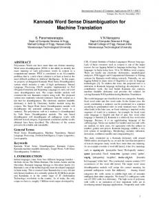
Figure 4: Individual basic classifiers’ contribution to the final classifier combination performance.
�
the combination classifier estimates the sense prob� � ��� � ���� �� � � � �. abilities,
��
� �
� � � �
6.2
Individual Systems Contribution to Combination An interesting issue pertaining to classifier combination is what is the marginal contribution to final combined performance of the individual classifier. A suitable measure of this contribution is the difference in performance between a combination system’s behavior with and without the particular classifier. The more negative the accuracy difference on omission, the more valuable the classifier is to the ensemble system. Figure 4(a) displays the drop in performance obtained by eliminating in turn each classifier from the 6-way combination, across four languages, while Figure 4(b) shows the contribution of each classifier on the SENSEVAL 2 English data for different training sizes (10%-80%)8 . Note that the classifiers with the greatest marginal contribution to the combined system performance are not always the best single performing classifiers (Table 3(b)), but those with the most effective original exploitation of the common feature space. On average, the classifier that contributes the most to the combined system’s performance is the TBL classifier, with an average improvement of �
� across the 4 languages. Also, note that TBL and DL offer the greatest marginal contribution on smaller training sizes (Figure 4(b)).
�
6.3 Performance on Test Data At all points in this article, experiments have been based strictly on the original SENSEVAL 1 and SEN SEVAL 2 training sets via cross-validation. The official SENSEVAL 1 and SENSEVAL 2 test sets were 8
The latter graph is obtained by sampling repeatedly a prespecified ratio of training samples from 3 of the 5 crossvalidation splits, and testing on the other 2.
unused and unexamined during experimentation to avoid any possibility of indirect optimization on this data. But to provide results more readily comparable to the official benchmarks, a single consensus system was created for each language using linear average stacking on the top three classifier combination methods in Table 3 for conservative robustness. The final frozen consensus system for each language was applied once to the SENSEVAL test sets. The fine-grained results are shown in Table 5. For each language, the single new stacked combination system outperforms the best previously reported SENSEVAL results on the identical test data9 . As far as we know, they represent the best published results for any of these five SENSEVAL tasks.
7 Conclusion In conclusion, we have presented a comparative evaluation study of combining six structurally and procedurally different classifiers utilizing a rich common feature space. Various classifier combination methods, including count-based, rank-based and probability-based combinations are described and evaluated. The experiments encompass supervised lexical sample tasks in four diverse languages: English, Spanish, Swedish, and Basque. 9 To evaluate systems on the full disambiguation task, it is appropriate to compare them on their accuracy at 100% testdata coverage, which is equivalent to system recall in the official SENSEVAL scores. However, it can also be useful to consider performance on only the subset of data for which a system is confident enough to answer, measured by the secondary measure precision. One useful byproduct of the CBV method is the confidence it assigns to each sample, which we measured by the number of classifiers that voted for the sample. If one restricts system output to only those test instances where all participating classifiers agree, consensus system performance is 83.4% precision at a recall of 43%, for an F-measure of 56.7 on the SENSEVAL 2 English lexical sample task. This outperforms the two supervised SENSEVAL 2 systems that only had partial coverage, which exhibited 82.9% precision at a recall of 28% (F=41.9) and 66.5% precision at 34.4% recall (F=47.9).
SENSEVAL 1
Mean Official SENSEVAL Systems Accuracy Best Previously Published SENSEVAL Accuracy Best Individual Classifier Accuracy New (Stacking) Accuracy
English 73.1�2.9 77.1% 77.1% 79.7%
SENSEVAL 2
English 55.7�5.3 64.2% 62.5% 66.5%
Sense Classification Accuracy Spanish Swedish Basque 59.6�5.0 58.4�6.6 74.4�1.8 71.2% 70.1% 75.7% 69.6% 68.6% 75.6% 72.4% 71.9% 76.7%
Table 5: Final Performance (Frozen Systems) on SENSEVAL Lexical Sample WSD Test Data
The experiments show substantial variation in single classifier performance across different languages and data sizes. They also show that this variation can be successfully exploited by 10 different classifier combination methods (and their metavoting consensus), each of which outperforms both the single best classifier system and standard classifier combination models on each of the 4 focus languages. Furthermore, when the stacking consensus systems were frozen and applied once to the otherwise untouched test sets, they substantially outperformed all previously known SENSEVAL 1 and SEN SEVAL 2 results on 4 languages, obtaining the best published results on these data sets.
8 Acknowledgements The authors would like to thank Noah Smith for his comments on an earlier version of this paper, and the anonymous reviewers for their useful comments. This work was supported by NSF grant IIS-9985033 and ONR/MURI contract N00014-01-1-0685.
References A. Berger. 1996. Convexity, maximum likelihood and all that. http://www.cs.cmu.edu/afs/cs/user/aberger/ www/ps/convex.ps. E. Brill and J. Wu. 1998. Classifier combination for improved lexical disambiguation. In Proceedings of COLING-ACL’98, pages 191–195. E. Brill. 1995. Transformation-based error-driven learning and natural language processing: A case study in part of speech tagging. Computational Linguistics, 21(4):543–565. S. Cucerzan and D. Yarowsky. 2000. Language independent minimally supervised induction of lexical probabilities. In Proceedings of ACL-2000, pages 270–277. S. Cucerzan and D. Yarowsky. 2002. Augmented mixture models for lexical disambiguation. In Proceedings of EMNLP-2002. W. Daelemans, A. van den Bosch, and J. Zavrel. 1999. Timbl: Tilburg memory based learner - version 1.0. Technical Report ilk9803, Tilburg University, The Netherlands. A.P. Dempster, N.M. Laird, , and D.B. Rubin. 1977. Maximum likelihood from incomplete data via the EM algorithm. Journal of the Royal statistical Society, 39(1):1–38. P. Edmonds and S. Cotton. 2001. SENSEVAL -2: Overview. In Proceedings of SENSEVAL -2, pages 1–6. N. Fuhr. 1989. Optimum polynomial retrieval funcions based on the probability ranking principle. ACM Transactions on Information Systems, 7(3):183–204. W. Gale, K. Church, and D. Yarowsky. 1992. A method for disambiguating word senses in a large corpus. Computers and the Humanities, 26:415–439.
J. Henderson and E. Brill. 1999. Exploiting diversity in natural language processing: Combining parsers. In Proceedings on EMNLP99, pages 187–194. A. Kilgarriff and M. Palmer. 2000. Introduction to the special issue on senseval. Computer and the Humanities, 34(1):1-13. A. Kilgarriff and J. Rosenzweig. 2000. Framework and results for English Senseval. Computers and the Humanities, 34(1):15-48. C.D. Manning and H. Schütze. 1999. Foundations of Statistical Natural Language Processing. MIT Press. G. Ngai and R. Florian. 2001. Transformation-based learning in the fast lane. In Proceedings of NAACL’01, pages 40–47. T. Pedersen. 1998. Naïve Bayes as a satisficing model. In Working Notes of the AAAI Symposium on Satisficing Models. T. Pedersen. 2000. A simple approach to building ensembles of naive bayesian classifiers for word sense disambiguation. In Proceedings of NAACL’00, pages 63–69. M. P. Perrone and L. N. Cooper. 1993. When networks disagree: Ensemble methods for hybrid neural networks. In R. J. Mammone, editor, Neural Networks for Speech and Image Processing, pages 126–142. Chapman-Hall. E. F. Tjong Kim Sang, W. Daelemans, H. Dejean, R. Koeling, Y. Krymolowsky, V. Punyakanok, and D. Roth. 2000. Applying system combination to base noun phrase identification. In Proceedings of COLING 2000, pages 857–863. M. Stevenson and Y. Wilks. 2001. The interaction of knowledge sources in word sense disambiguation. Computational Linguistics, 27(3):321–349. K. Tumer and J. Gosh. 1995. Theoretical foundations of linear and order statistics combiners for neural pattern classifiers. Technical Report TR-95-02-98, University of Texas, Austin. H. van Halteren, J. Zavrel, and W. Daelemans. 1998. Improving data driven wordclass tagging by system combination. In Proceedings of COLING-ACL’98, pages 491–497. H. van Halteren, J. Zavrel, and W. Daelemans. 2001. Improving accuracy in word class tagging through the combination fo machine learning systems. Computational Linguistics, 27(2):199–230. L. Xu, A. Krzyzak, and C. Suen. 1992. Methods of combining multiple classifires and their applications to handwriting recognition. IEEE Trans. on Systems, Man. Cybernet, 22(3):418–435. D. Yarowsky and R. Florian. 2002. Evaluating sense disambiguation performance across diverse parameter spaces. To appear in Journal of Natural Language Engineering. D. Yarowsky and R. Wicentowski. 2000. Minimally supervised morphological analysis by multimodal alignment. In Proceedings of ACL-2000, pages 207–216. D. Yarowsky. 1996. Homograph disambiguation in speech synthesis. In J. Olive J. van Santen, R. Sproat and J. Hirschberg, editors, Progress in Speech Synthesis, pages 159–175. Springer-Verlag.