Modeling, Control and Self-Sensing of Dielectric

POLITECNICO DI BARI SCUOLA INTERPOLITECNICA DI DOTTORATO Doctoral Program in Electrical and Information Engineering – XXVIII cycle

Final Dissertation

Modeling, Control and Self-Sensing of Dielectric Elastomer Actuators

Ph.D. Candidate: Gianluca Rizzello

Supervisors Prof. David Naso (Politecnico di Bari) Prof. Stefan Seelecke (Universität des Saarlandes)

Coordinator of the Research Doctorate Prof. Vittorio M.N. Passaro (Politecnico di Bari)

April 2016

“They don’t sleep anymore on the beach” Godspeed You! Black Emperor - Sleep

Acknowledgements I would like to thank my advisor Prof. David Naso from Politecnico di Bari for his constant guidance, for supporting my ideas through my Ph.D studies, and for giving me the opportunity of practicing my teaching skills. I would also like to thank my co-advisor Prof. Stefan Seelecke from Universität des Saarlandes for hosting me in his laboratory, for motivating my interest in smart materials with many scientific discussions, and for letting me support his teaching activities. I personally thank my collegue and friend Micah Hodgins for his constant support with experimental activities, and for inspiring me with his great ideas concerning the design of Dielectric Elastomer actuators. I would also like to thank my colleague and friend Dr. Leonardo Riccardi for the numerous discussions we had on the field of control of smart materials, and for stimulating my interest in the area of robust control. I am personally grateful to all the professors and researchers who have supported my work and stimulated my interest in research in various way: Prof. Francesco Cupertino, Prof. Biagio Turchiano, Dr. Giulio Binetti, Giuseppe Cofano, Francesco Ferrante, Giulia Giordano, Alessandra Guagnano, and many others. A special thanks goes also to all the students who have collaborated with me with their thesis projects, in particular to Diego Di Leo and Marco Lacitignola, whose company and companionship made my experience in Saarbr¨ ucken an unforgettable one. Last but not least, I want to thank my girlfriend Filomena for her precious love and support, and for continuously encouraging me.

Contents Acknowledgements

v

1 Introduction 1.1 Motivation . . . . . . . . . . . . . . . . . . . . . . . . . . . . . . . . . 1.2 Contribution . . . . . . . . . . . . . . . . . . . . . . . . . . . . . . . .

1 1 3

2 Dielectric Elastomers (DEs) 2.1 DE material . . . . . . . . . . . . . . . 2.2 DEs applications . . . . . . . . . . . . 2.2.1 DE Actuators (DEAs) . . . . . 2.2.2 DE Sensors (DESs) . . . . . . . 2.2.3 DE Generators (DEGs) . . . . . 2.3 Case of study: circular membrane DEA 2.3.1 Actuator description . . . . . . 2.3.2 Effects of the biasing system . . 2.3.3 Experimental setup . . . . . . .

. . . . . . . . .

. . . . . . . . .

. . . . . . . . .

. . . . . . . . .

. . . . . . . . .

. . . . . . . . .

. . . . . . . . .

. . . . . . . . .

. . . . . . . . .

. . . . . . . . .

. . . . . . . . .

. . . . . . . . .

. . . . . . . . .

. . . . . . . . .

. . . . . . . . .

7 7 8 9 12 14 17 18 18 20

3 Modeling 3.1 Modeling problem statement . . . . . . . . . 3.2 Literature review . . . . . . . . . . . . . . . 3.3 DE material model . . . . . . . . . . . . . . 3.3.1 Free-energy based model . . . . . . . 3.3.2 Selection of material model . . . . . 3.3.3 A special case of DE material model 3.4 DE actuator model . . . . . . . . . . . . . . 3.4.1 Biasing system model . . . . . . . . . 3.4.2 DE membrane model . . . . . . . . . 3.4.3 Electrical dynamics model . . . . . . 3.4.4 Complete model . . . . . . . . . . . . 3.5 Model validation . . . . . . . . . . . . . . . 3.5.1 DEA + Linear Biasing Spring (LBS)

. . . . . . . . . . . . .

. . . . . . . . . . . . .

. . . . . . . . . . . . .

. . . . . . . . . . . . .

. . . . . . . . . . . . .

. . . . . . . . . . . . .

. . . . . . . . . . . . .

. . . . . . . . . . . . .

. . . . . . . . . . . . .

. . . . . . . . . . . . .

. . . . . . . . . . . . .

. . . . . . . . . . . . .

. . . . . . . . . . . . .

. . . . . . . . . . . . .

25 26 29 31 33 39 48 50 51 53 62 66 70 70

vii

. . . . . . . . .

. . . . . . . . .

3.5.2 3.5.3 3.5.4

DEA + Nonlinear Biasing Spring (NBS) + LBS . . . . . . . . 81 Comparison of different biasing systems . . . . . . . . . . . . . 83 Effects of quadratic nonlinearity on mechanichal resonance . . 86

4 Control 4.1 Control problem statement . . . . . . . . . . . . . . . . . . . . . . . 4.2 Literature review . . . . . . . . . . . . . . . . . . . . . . . . . . . . 4.3 Systematic approaches: feedforward and feedback linearization . . . 4.3.1 Feedforward . . . . . . . . . . . . . . . . . . . . . . . . . . . 4.3.2 Feedback linearization . . . . . . . . . . . . . . . . . . . . . 4.4 Position control for small deformations . . . . . . . . . . . . . . . . 4.4.1 Linear control based on model linearization . . . . . . . . . 4.4.2 Model linearization with square root compensator . . . . . . 4.5 Position control for large deformations . . . . . . . . . . . . . . . . 4.5.1 DEA model reformulation as quasi-LPV . . . . . . . . . . . 4.5.2 LMI-based PID control, dynamic reduction method . . . . . 4.5.3 LMI-based PID control, quasi zero-pole cancellation method 4.5.4 LMI-based linear control, norm-based specification . . . . . 4.6 Control of DEA operating against an external system . . . . . . . . 4.6.1 DEA interacting with a structured environment . . . . . . . 4.6.2 DEA interacting with an unstructured environment . . . . . 4.7 Results . . . . . . . . . . . . . . . . . . . . . . . . . . . . . . . . . . 4.7.1 Position control for small deformations, DEA + LBS . . . . 4.7.2 Position control for large deformations, DEA + NBS + LBS

. . . . . . . . . . . . . . . . . . .

5 Self-sensing 5.1 Self-sensing problem statement . . . . . . . . . . . . . . . . . 5.2 Literature review . . . . . . . . . . . . . . . . . . . . . . . . . 5.3 Self-sensing algorithm . . . . . . . . . . . . . . . . . . . . . . . 5.3.1 Reconstructing displacement from electrical parameters 5.3.2 Input voltage signal for self-sensing . . . . . . . . . . . 5.3.3 Online estimation based on full model . . . . . . . . . 5.3.4 Online estimation based on simplified model . . . . . . 5.3.5 Filtering . . . . . . . . . . . . . . . . . . . . . . . . . . 5.3.6 Complete self-sensing algorithm . . . . . . . . . . . . . 5.4 Results . . . . . . . . . . . . . . . . . . . . . . . . . . . . . . . 5.4.1 Sensing . . . . . . . . . . . . . . . . . . . . . . . . . . 5.4.2 Self-sensing . . . . . . . . . . . . . . . . . . . . . . . .

173 . 173 . 176 . 177 . 178 . 179 . 180 . 183 . 185 . 187 . 188 . 188 . 194

viii

. . . . . . . . . . . .

. . . . . . . . . . . .

. . . . . . . . . . . .

89 91 94 97 97 98 101 102 108 111 112 114 119 132 137 138 142 150 150 153

6 Self-sensing based control 6.1 Self-sensing based control architecture . . . . 6.2 Results . . . . . . . . . . . . . . . . . . . . . . 6.2.1 Self-sensing based position control . . . 6.2.2 Self-sensing based position control with 6.2.3 Self-sensing based interaction control .

. . . . . . . . . . . . . . . . . . . . . . . . . . . . . . an external load . . . . . . . . . .

. . . . .

. . . . .

7 Conclusion

. . . . .

199 199 201 201 208 212 221

A DEA model passivity and port-Hamiltonian A.1 DEA total energy . . . . . . . . . . . . . . . A.2 DEA as a passive system . . . . . . . . . . . A.3 DEA as a port-Hamiltonian system . . . . .

representation . . . . . . . . . . . . . . . . . . . . . . . . . . . . . . . . . . . . . . .

B Introduction to LMI and LPV systems B.1 LMI problems . . . . . . . . . . . . . . . . . . . . . . . B.1.1 LMI notation . . . . . . . . . . . . . . . . . . . B.1.2 Useful LMI properties . . . . . . . . . . . . . . B.1.3 Standard LMI problems . . . . . . . . . . . . . B.2 LPV systems . . . . . . . . . . . . . . . . . . . . . . . B.3 Analysis of LPV systems via LMI . . . . . . . . . . . . B.3.1 Quadratic stability . . . . . . . . . . . . . . . . B.3.2 Quadratic stability with exponential decay rate B.3.3 H2 performance . . . . . . . . . . . . . . . . . . B.3.4 Generalized H2 performance . . . . . . . . . . . B.3.5 H∞ performance . . . . . . . . . . . . . . . . . B.4 Feedback control of LPV systems via LMI . . . . . . . B.4.1 Quadratic stability . . . . . . . . . . . . . . . . B.4.2 Quadratic stability with exponential decay rate B.4.3 H2 performance . . . . . . . . . . . . . . . . . . B.4.4 Generalized H2 performance . . . . . . . . . . . B.4.5 H∞ performance . . . . . . . . . . . . . . . . . B.4.6 Multiobjective control . . . . . . . . . . . . . . B.4.7 A special case of static output feedback . . . . .

. . . . . . . . . . . . . . . . . . .

. . . . . . . . . . . . . . . . . . .

. . . . . . . . . . . . . . . . . . .

. . . . . . . . . . . . . . . . . . .

. . . . . . . . . . . . . . . . . . .

. . . . . . . . . . . . . . . . . . .

. . . . . . . . . . . . . . . . . . .

225 . 225 . 228 . 231 235 . 235 . 235 . 236 . 238 . 239 . 245 . 245 . 248 . 249 . 250 . 251 . 252 . 253 . 253 . 253 . 254 . 254 . 255 . 256

C Boundedness of state variables

259

Bibliography

265

ix

Chapter 1 Introduction 1.1

Motivation

Electro-Active Polymers (EAPs) represent an innovative class of smart materials which exhibit relatively large deformations when solicited by electrical or chemical stimuli [1]. Dielectric EAPs (DEAPs), most commonly referred to as Dielectric Elastomers (DEs), represent a class of EAPs consisting of a film of elastic polymeric material covered on both sides by compliant electrodes. When a voltage is applied to the electrodes, the resulting electric field generates a compressive stress that produces a controllable deformation [2]. This deformation can be in some cases one or two orders of magnitude larger than the one obtained by other smart materials (e.g., piezoelectric ceramics, shape memory alloys). Large deformation (> 100% in many cases), low production cost, low power requirement, high energy density, and comparatively high bandwidth make DEs an attractive alternative for the development of a new generation of mechatronic devices. In fact, several prototypes of pumps [3, 4, 5, 6, 7], valves [8, 9, 10], loudspeakers [11, 12], robots [13, 14, 15], flapping wing insects [16, 17], optical positioning systems [18, 19, 20], micro-positioning stages [21], pressure or deformation sensors [22, 23, 24, 25], and energy harvesters [26, 27, 28, 29, 30] have been presented in recent literature. On the other hand, there are many technological issues that still need to be properly addressed in order to make this material competitive in industrial applications, such as the amount of voltage needed to obtain a significant deformation, the strong nonlinearities in the input-output characteristics, and the dependence of the response on environmental conditions and fatigue. The main focus of this thesis is on DE Actuator (DEA) systems. In order to efficiently exploit the many features of DE devices, their complex dynamic behavior needs to be properly characterized and described by means of mathematical models. Actuator simulation, design of high-precision and high-speed model-based control 1

1 – Introduction

systems, optimization of the actuator design for specific applications, and minimization of the energy consumption are among the many tasks that can be accomplished by means of an accurate model. Another attractive feature of DEAs is the possibility to perform self-sensing during actuation, which means that the elastomer is used as an actuator and a sensor simultaneously. In principle, a self-sensing actuator can be controlled in closed loop without requiring additional electromechanical transducers, thus increasing the compactness and reducing the cost of the overall system. In order to achieve self-sensing, the complex electro-mechanical coupling existing in the material needs to be accurately characterized and modeled. Recent literature presents a significant amount of works on characterization, on constitutive modeling of DE materials, and on design of DE-based devices. Nevertheless, the development of a systematic framework for control-oriented modeling and model-based feedback control of DEA systems is still an open research topic. Motivated by the growing interest in DE technology for industrial-oriented applications, the main objective of this thesis is the development of model-based feedback control systems which allow to drive DEAs fast, accurately, and in a self-sensing fashion. In order to achieve this goal, three major aspects need to be investigated: • Modeling: to understand the complex dynamics of the overall actuator system, including the numerous nonlinearities characterizing the response of the material, and to describe them by means of a model; • Control: starting from an accurate mathematical description of the system, to develop feedback control algorithms which compensate the nonlinearities and achieve closed loop positioning with some desired dynamic performance (e.g., stability, bandwidth, robustness); • Self-sensing: to exploit the unique self-sensing feature of the material by means of real-time estimation algorithms, and to implement the feedback control strategies in combination with self-sensing estimation, achieving a socalled sensorless control scheme. By combining the results presented in recent literature with the work developed by the author, the main idea behind this thesis is the development of a unified mathematical framework which can be used to address modeling, control, and selfsensing problems for a large family of DEA systems. Once a solution for such a problems is available, it will lead to a new generation of compact, energy-efficient, and low-cost actuator devices capable of operating in closed loop without additional electromechanical transducers, reaching performance which are not available with current transduction technologies. Artificial muscles, copper-free electromechanical transducers, low cost distributed motion and force actuators represent some of the 2

1.2 – Contribution

most promising fields which would benefit from DE technology. In all of these applications, the use of feedback control will help to significantly improve the performance of the material by compensating its nonlinearities. At present, the remarkable potential of DEAs remains largely unexploited due to some current limitations of the material itself (high voltage requirement, low resistance to fatigue). However, considering the recent advances of material science, it is foreseeable that these limitations will be overcame in a next future, and at that time smart control algorithms will then be already available to let the material operate effectively and reliably in real-life conditions. This thesis has been developed within a collaboration between the Automation and Robotics Lab in Politecnico di Bari, Bari, Italy, and the intelligent Material Systems Lab in Universität des Saarlandes, Saarbr¨ ucken, Germany. The theory and the experimental results presented in this thesis have also been reported in the author’s papers [31, 32, 33, 34, 35, 36, 37, 38, 39, 40, 41, 42, 43, 44, 45].

1.2

Contribution

The organization of the thesis and the contributions of each chapter are summarized as follows. Chapter 2: In this chapter, the DE material is first introduced. Subsequently, the operating principle of the material and its use in the three principal areas of applications, namely actuators, sensors, and energy harvesters, is presented. Several examples of DE-based devices presented in recent literature are also discussed. After that, a circular membrane DEA with a bi-stable biasing system is presented. Such an actuator represents the principal case of study used to validate the theory developed in this thesis. A study of the effects of the biasing system on the overall membrane actuator performance is then presented. Finally, the chapter is concluded with the description of the test rig used for experimental investigation. Chapter 3: This chapter introduces first the general problem of modeling a DEA system. The principal input and output quantities of the model are initially defined. Then, the overall structure of the model is decomposed into its principal dynamics, that are biasing system, DE membrane, and electrical dynamics. After providing a brief review of recent works dealing with dynamic modeling of DEAs, the chapter discusses in great details the modeling of each of the three principal dynamics of the system. The major focus is on the dynamics of the material itself, which represents the most complex part of the overall system. A nonlinear viscoelastic model is proposed for describing a large class of DE membranes. Subsequently, the general model structure is used for describing the circular membrane DEA under investigation. The theory is validated by means of several experimental results. To the author’s best knowledge, the results presented in this chapter represent the first 3

1 – Introduction

experimental validation of a DEA model capable of predicting electrical response, mechanical response, and the effects of different biasing systems simultaneously (either linear or nonlinear), in a relatively large frequency range. The work in this chapter has also been reported in journal papers [31, 33] and in conference paper [34, 36, 41]. Chapter 4: In this chapter, the model presented in Chapter 3 is used to develop several feedback control strategies for the DEA system. This chapter mainly focuses on two control paradigms, namely position and interaction control. The control problem is initially stated, and a review of the approaches proposed in recent literature is provided. Then, starting from the general DEA model formulation, initial solutions based on feedforward and feedback linearization are presented. Such solutions are sensitive to model parameters, and in particular the latter requires a relatively high amount of real-time computational effort for its implementation. For this reason, the focus of the subsequent sections is shifted towards robust linear control laws, e.g., PID or linear state feedback, which are more attractive in terms of low implementation effort. A first method based on model linearization is described and used to tune a PID control law. This approach is suitable for applications in which the DEA exhibits small deformations around an operating point, e.g., when the overall actuator is biased with a linear spring. Subsequently, a modified controller, namely a PID cascaded with a square root, is introduced and compared with the standard PID, and it is shown how this simple modification permits to significantly improve the closed loop performance. Afterwards, the chapter focuses on the control of DEA in case of large deformations, that is when the DEA is biased with a bi-stable biasing system which results into an hysteretic voltage-displacement response. In this case, it is foreseeable to assume that a controller tuned according to a linearization approach would lead to unsatisfactory performance. For this reason, a new controller design methodology which ensures guaranteed stability and performance in the entire operating range is presented. The key idea behind the new method is the reformulation of the strong nonlinearities of the original model in a quasi-Linear Parameter Varying (LPV) system. Such a reformulation permits to address the design of a linear control law, e.g., PID or partial state feedback, ensuring robust stability and performance with respect to nonlinearities by using Linear Matrix Inequality (LMI) optimization. The design of partial state feedback control laws based on LMI optimization is challenging due to lack of convexity. Therefore, new strategies are presented in this thesis to address the design problem for the particular class of LPV models describing the DEA. To the author’s best knowledge, the proposed method based on quasi-LPV framework represents the first systematic analytical approach for robust PID control of DEA systems. For concluding the chapter, the control of a DEA interacting with an external system is also considered. Two main cases are discussed, namely DEA interacting with a structured and an unstructured environment, and a general solution based on LMI optimization is 4

1.2 – Contribution

proposed for both cases. The work in this chapter has also been reported in journal papers [32, 41] and in conference papers [35, 37, 38, 39]. Chapter 5: While the use of the DEA model for feedback control design is widely discussed in Chapter 4, the development of a model-based self-sensing strategy is the main focus of this chapter. The problem of self-sensing for DEA is initially introduced, and an overview of the most significant results presented in recent literature is provided. Subsequently, a self-sensing approach based on online estimation algorithms and digital filtering techniques is discussed in details. The main advantages of the proposed methodology are the remarkable accuracy and the relatively low implementation effort, which makes the algorithm suitable for real-time implementation on a microcontroller. Moreover, the method requires only voltage and current measurements. Since such quantities are typically available from the same electronic circuit used to drive the actuator, no special hardware architectures or additional sensors are usually required for its implementation (e.g., Pulse Width Modulation converters, charge sensors, peak or phase detection methods). To the author’s best knowledge, the approach presented in this chapter represents the first self-sensing method for DEAs based on time-domain identification and filtering techniques requiring voltage and current measurements only. An experimental campaign is also performed in order to evaluate the performance of the algorithm in a large set of operating conditions. The work in this chapter has also been reported in journal paper [43] and in conference paper [40]. Chapter 6: This chapter shows how the control methods developed in Chapter 4 are still capable to perform satisfactorily when the feedback of the output signal is provided by the self-sensing algorithm discussed in Chapter 5. An extensive experimental campaign is performed, in order to compare the closed loop performance achieved in case of sensor-based and self-sensing based displacement feedback. To the author’s best knowledge, this thesis presents the first direct comparison between sensor-based and self-sensing control of DEAs, for a comparatively high closed loop bandwidth, and for a wide set of reference signals. Subsequently, the self-sensing technique is used to implement the interaction control schemes presented at the end of Chapter 4. The resulting closed loop architecture allows to control the DEA stiffness by requiring only contact force measurement. This can be potentially advantageous in applications in which it is difficult to accurately measure the deformation of the membrane (e.g., when the actuator interacts with an external load), but it is relatively simpler to measure the contact force. To the author’s best knowledge, the work presented in this chapter is the first attempt which combines self-sensing and interaction control techniques for DEAs. The work in this chapter has also been reported in journal papers [42, 44] and in conference paper [45]. Chapter 7: This chapter concludes the thesis by discussing some possible future research directions in the area of modeling, control, and self-sensing of DEAs.

5

Chapter 2 Dielectric Elastomers (DEs) This chapter aims at introducing some general concepts on Dielectric Elastomer (DE) transducers. The main focus is on DEs operating principle and applications, with a particular emphasis on DE actuators. Details on chemical structure and fabrication of the material will not be discussed for conciseness. The principal characteristics of DE material are initially discussed in Section 2.1. The electro-mechanical coupling existing in the material can be exploited for the fabrication of several kind of mechatronic devices, ranging from DE Actuators (DEAs) to DE Sensors (DESs) and DE Generators (DEGs). The physical principles behind these applications are briefly discussed in Section 2.2. A list of several prototypes published in recent literature is also discussed. Finally, Section 2.3 concludes the chapter with the description of the experimental case of study of this thesis, consisting of a circular membrane DEA combined with several kind of biasing elements including linear and bi-stable springs. The effect of the biasing system on the overall actuator performance is explained in details, and the advantages of adopting a bi-stable rather than a linear biasing system are discussed.

2.1

DE material

A DE consists of a polymeric membrane (e.g., silicone, VHB acrylic, natural rubber) with compliant electrodes (e.g., carbon grease, graphene, carbon nanotubes) applied on both sides of the external surface, forming a compliant capacitor. DEs can be used as electromechanical transducers, enabling the conversion from electrical to mechanical energy and vice versa. In fact, when a voltage is applied at the electrode surface, electrostatic forces generate a compression of the membrane and a consequent expansion of its area. Conversely, if a DE membrane is deformed by an external force, its electrical impedance changes accordingly. Such principles can be naturally exploited in actuation, sensing, and energy harvesting applications. 7

2 – Dielectric Elastomers (DEs)

Value Acrylics DE Silicones DE 380 120 8.2 3 >50 >50 3.4 0.75 440 350 4.5÷4.8 2.5÷3 0.005 80 >80 >107 >107 -10÷90 -100÷260

Property Maximum actuation strain Maximum actuation stress Maximum frequency response Maximum energy density Maximum electric field Relative permittivity (at 1 kHz) Dielectric loss factor (at 1 kHz) Mechanical loss factor Young Modulus Maximum electro-mechanical coupling Maximum overall efficiency Durability Operating range Table 2.1.

Unit [%] [MPa] [kHz] [MJ/m3 ] [MV/m] [-] [-] [-] [MPa] [-] [%] [cycles] [◦ C]

Performance of best acrylics and silicones DEs [2].

The most attractive feature of DEs is represented by their relatively large strain which can be, in many cases, larger than 100% [46]. Other than that, DEs exhibit further attractive characteristics such as high energy density, high efficiency, fast response time, low power consumption, high flexibility, and low cost. On the other hand, the major limitations of DE technology are represented by the high electric field requirement for achieving a significant electromechanical activation (larger than 10 MV/m and close to the breakdown level, resulting in voltage values of the order of kV), the relatively low forces, the strongly nonlinear input-output behavior, and the sensitivity to temperature, humidity, and fatigue. To overcome the most critical limitations of the material in order to allow the realization of reliable and low-cost devices based on DEs, a significant amount of research is being conducted in the area of material optimization, with the dual goal of reducing the voltage required for electromechanical activation and increasing the lifetime of the material [47, 48]. A list of figures of merit of the best DE transducers are reported in Table 2.1 [2].

2.2

DEs applications

The transduction principle of DEs can be exploited to use the polymer either as an electro-mechanical actuator, sensor or generator. The way these three operating modes can be achieved by means of DE technology is discussed in the following. 8

2.2 – DEs applications

DE membrane

Maxwell Stress + -

Electrodes (a)

+ -

+ -

+ -

+ -

(b)

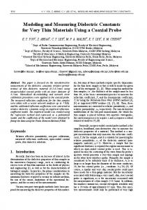
Figure 2.1. DE electro-mechanical transduction principle, voltage OFF (a), and voltage ON (b).

2.2.1

DE Actuators (DEAs)

A DEA is a mechatronic device capable of converting an applied voltage into a motion. The operating principle of a DEA is relatively simple, and is shown in Figure 2.1. When a voltage is applied to the electrodes, charges flow from an electrode to the other through an external circuit. The combination of attractive electrostatic forces between charges of different sign on opposite electrodes and repulsive electrostatic forces between charges of equal sign on the same electrode result in a membrane squeezing, which causes a reduction in thickness and a consequent expansion in area. The equivalent compressive stress induced by the electric field is known in the literature as Maxwell stress [2] and is given by σM ax = −ǫ0 ǫr E 2 ,

(2.1)

where σM ax is the Maxwell stress, which is proportional by the void permittivity ǫ0 and the elastomer relative permittivity ǫr to the square of the electric field E resulting from the application of an external voltage. The Maxwell stress is directed according to the electric field, and its sign is always negative as the film is being compressed. Equation (2.1) represents the electro-mechanical transduction principle of a DE, and puts also in evidence its nonlinear nature. By replacing the electric field E with the ratio between applied voltage vDE and membrane thickness z, equation (2.1) can be equivalently rewritten as σM ax = −ǫ0 ǫr

vDE z

2

.

(2.2)

From equation (2.1), we see that the electrically induced stress which is responsible for the electro-mechanical transduction increase linearly with the material permittivity ǫr and quadratically with the applied voltage vDE . A very simple model of a DEA can be derived from the the Maxwell stress equation in (2.2). As a first approximation, we can assume that the material behaves as a linear spring. Then, the stress and the strain in the thickness direction, denoted 9


as σz and εz respectively, are related by σz = Y ε z ,

(2.3)

where Y is the Young modulus of the material. If we express the actual thickness z as a function of the undeformed thickness z0 and the thickness strain as z = z0 (1 + εz ),

(2.4)

by assuming σz = σM ax and replacing (2.3) and (2.4) in (2.2) we obtain Y εz = −ǫ0 ǫr

vDE z0 (1 + εz )

2

.

(2.5)

By assuming small deformations (|εz | ≪ 1), equation (2.5) can be approximated as follows ǫr εz = −ǫ0 vDE 2 . (2.6) Y z0 2 As further step, we can express the thickness strain εz in terms of the in-plane strain εx (assuming isotropic deformations, that is εx = εy ) by using the incompressibility assumption (which is typically true for DE material) (1 + εx )2 (1 + εz ) = 1.

(2.7)

If deformations are small, equation (2.7) can be approximated as εx = −νεz .

(2.8)

where the Poisson’s ratio is ν = 0.5. The relationship between voltage and in-plane strain results then into ǫr εx = 2ǫ0 vDE 2 . (2.9) 2 Y z0 Equations (2.6) and (2.9) can be used to describe the basic behavior of a DEA operating in contraction (εz < 0) and expansion mode (εx > 0), respectively. Both equations highlight the fact that a larger strain can be obtained for the same voltage if the material permittivity is large and both Young modulus and initial thickness of the membrane are small. In practice, the thickness z0 cannot be made arbitrarily small as the resulting electric field would increase to values close to the material dielectric strength, thus compromising the stability of the system. Moreover, a smaller thickness would also make the manufacturing process more complicated, and compromise the lifetime of the material as well. The relative permittivity ǫr and the Young modulus Y represent constitutive parameters which can be tuned, up to certain limits, in the 10


material manufacturing process stage. As previously stated, in order to increase the actuation stroke Y needs to be reduced, while ǫr must be as large as possible. However, decreasing the material stiffness leads to a reduction of the actuation force, while increasing the permittivity results in an increase of the capacitance with a consequent increment of both (reactive) power requirement and electrical response time. In case of membrane DEAs, another possible way to increase the stroke consists of preloading the polymeric film with a mechanical biasing system. The mechanical biasing is of fundamental importance in determining the performance DEA systems, and its role is discussed in details in Section 2.3.2. Considering typical values of parameters, i.e., Y about 1 MPa, ǫr about 3, and z0 about 50 µm, voltage levels of the order of several kV are typically requested in order to achieve a significantly large strain. Such voltage values tend to generate electric field that are close to the dielectric strength of the material. The high voltage requirement remains nowadays the major limitation of DE technology in actuator applications. Despite the high voltage limitation, however, the current consumption is relatively small (order of µA), resulting in a power requirement of the order of mW. Other than high deformation and low-power consumption, the main advantages of DEAs are their flexibility and scalability, which enable the manufacturing of several actuator configurations. In fact, the actuation principle described previously for an elementary membrane can be further extended and characterized for many possible geometries, generating a large varieties of actuation modes [49, 50]. A number of DEA configurations have been proposed in recent literature, including extender actuators [51], diaphragm actuators [52], helical actuators [53], unimorph actuators [54], bimorph actuators [55], framed actuators [56], circular actuators [57], roll actuators [58], cylindrical actuators [59], diamond actuators [60], bow-tie actuators [61], spider actuators [62], out-of-plane actuators [63], rotary actuators [64], and stack actuators [65]. Several prototypes of DEA devices have been proposed for a large variety of applications, ranging from standard industrial ones, like robots or valves, to less conventional ones, like tunable lens elements and loudspeakers. In the following, some notable examples of DEAs presented in recent literature are shortly overviewed. In [14], a DE-driven hyper-redundant robot manipulator is presented. The system has the advantages of being potentially miniaturizable for applications such as biomedical devices or space system components. The authors show how to achieve improved performance by incorporating in the overall system passive elastic elements. In [10], Giousouf and Kovacs develop different designs for pneumatic valves based on stacked DEA. The authors perform an experimental measurement of the actuator force and stroke, and discuss also benefits and challenges of using DE technology in 11


such applications. The performance analysis of a DEA in high-precision positioning applications is investigated in [21]. The authors compare the proposed device with a micropositioning stage based on piezoelectrics, showing how the DEA could represent an attractive and low-cost alternative solution for high-precision positioning of optic components. It is remarked in many papers that DEs represent a particularly promising technology for the realization of artificial muscles. Several prototypes of bio-inspired robots using DEA artificial muscles which mimic insects and inchworms locomotion, flapping wings and serpentine manipulation are presented in [13], while an arm wrestling robot capable to mimic human muscles based on roll DEAs is presented in [66]. The modeling of a diaphragm DEA for potential use in a prosthetic blood pump is presented in [3]. The goal is to mimic the natural pumping chamber of the hearth by keeping a high volumetric efficiency. By means of simulations, the authors show that the device is capable of providing more than adequate volume displacement for the specific application. A bio-inspired lens with tunable focus made of DE is presented in [19]. The device consists of an elastomeric lens filled with fluid integrated with an annular DEA. The electrical activation of the actuator deforms the membrane and causes a change in the focal lens, allowing a compact, low-weight, low-power consumption, and fast optical device which mimics the architecture of human eye. The large bandwidth of DEA devices allows their applications in the field of acoustics, as well. An example is given by [12], which proposes a lightweight pushpull acoustic transducer based on dielectric elastomer films. In the paper, the authors show that the proposed push-pull driving configuration permits to reduce sensibly the harmonic distortion of the system. For concluding the section we point out that that, despite a significant amount of work has been done on the design of complex DEA devices, the systematic investigation of modeling and control problems for such systems remains, in many cases, still an unaddressed issue.

2.2.2

DE Sensors (DESs)

A DE is basically a compliant capacitor. When the membrane is deformed by an external force, the resulting capacitance changes according to the geometry. As the material can sustain significantly large deformations, the equivalent changes in capacitance are also quite high, making DE suitable for the design of capacitive sensors capable of measuring displacements or forces. Furthermore, the high flexibility of the elastomer permits to adapt a DES to a large variety of applications. 12


Undeformed

Deformed

Ael ,0

Ael

F z

z0

C0 = ε0εr

Ael ,0

C = ε0εr

z0

(a)

Figure 2.2.

F

Ael z

(b)

Elementary DES, undeformed (a), and deformed state (b).

An example of capacitance-displacement relationship for a DES can be obtained by using the parallel-plate capacitance formula to a thin DE membrane. If we consider the membrane in Figure 2.2, its capacitance in undeformed and deformed states, denoted as C0 and C respectively, is given by C 0 = ǫ0 ǫr

Ael,0 , z0

(2.10)

Ael , (2.11) z where Ael,0 and Ael represent the surface of the electrodes in undeformed and deformed configurations, respectively. If the membrane is incompressible, the volume V = Ael z = Ael,0 z0 remains constant. Therefore, (2.11) can be reformulated as C = ǫ0 ǫr

C = ǫ0 ǫr = ǫ0 ǫr

Ael z V z2

Ael,0 z0 z2 2 Ael,0 z0 = ǫ0 ǫr z0 z = ǫ0 ǫr

1 , (1 + εz )2

(2.12)

= C0 (1 + εx )4 ,

(2.13)

= C0

13


In order to obtain (2.12)-(2.13), incompressibility equation (2.7) was used. Note that the relationships between deformation and capacitance in (2.12) and (2.13) are nonlinear, thus the sensitivity of the resulting sensor depends on the measured strain value. We also point out that the principle which allows the use of DEs as sensors does not depend on Maxwell stress, but it relies on its nature of compliant capacitor. The capacitance is not the only electrical parameter of a DES which changes with deformation. The voltage drop on the electrodes and the leakage in the material, which can be modeled as equivalent resistive effects, make DESs behave as a RC circuit rather than as an ideal capacitor [67]. Reconstructing the DES deformation from its resistance rather than from its capacitance leads, in general, to a simplified design of the measurement electronic hardware. However, the resulting accuracy is generally lower than in case of capacitive measurement. Different prototypes of DES based on capacitance, resistance and overall electrical impedance have been proposed in recent literature. In [24], the capacitive sensing capabilities of a circular membrane DES are investigated. The proposed sensor, suitable for pumps and valves applications, is experimentally validated under mechanical loading conditions. Initial results of a dual sensing and actuating DE system are also presented. Several possible applications of DES technology are discussed in [23], including also a list of features and limitations. The authors propose some electronic circuits for measuring both capacitance and resistance of the material, and mention that both quantities can be used to reconstruct the deformation of the material. In [68], Goulbourne et al. present a self-sensing McKibben actuator based on a cylindrical DES. By measuring how the deformation of the actuator affects the electrical signals measured on the surface of the DES, the authors are able to perform in situ monitoring of strains and loads. In [69], a further setup for in situ monitoring based on DES is presented. Both capacitance and electrodes resistance are recorded and used to study relationship between the actuation signal and the resulting strain of the material. The use of DES to track movement of human hands is discussed in [70]. The authors present a simple method to measure charge and reconstruct the capacitance of the elastomer, which allows to monitor a large number of DESs simultaneously. A number of works investigate also the possibility of combining actuation and sensing capabilities of DEs, in order words to achieve self-sensing. However, the detailed discussion of the topic is postponed to Chapter 5.

2.2.3

DE Generators (DEGs)

The transduction mode used in a DEA can be reverted and used to convert mechanical energy into electrical, allowing to use the elastomer as a generator. The 14


F

F C1

(b)

F (a) Ł (e)

U out =

1 2 q 2C0

C0

q = C0 vDE ,0 + + + + + -

-

(d)

U in =

-

+ -

1 2 q 2C1

q = C1vDE ,1 + + + + (c)

F C1

C0

Figure 2.3. Operating principle of a DEG. The membrane initially undeformed (a), a mechanical load F is applied (b), electrical energy Uin is delivered by applying a charge q at voltage vDE,1 (c), the mechanical load F is removed (d), electrical energy Uout > Uin is absorbed by removing the charge q at voltage vDE,0 > vDE,1 , and the cycle is restarted (e).

operating principle of a DEG is illustrated in Figure 2.3, and consists of the following steps: (a) The DEG membrane is initially undeformed and electrically discharged. We denote as C0 its capacitance in the undeformed state; (b) An external mechanical force is applied, producing an expansion in area and a consequent reduction in thickness. We define the resulting capacitance in the deformed state as C1 , with C1 > C0 ; (c) A voltage vDE,1 is applied to the electrodes, and delivers a charge q = C1 vDE,1 ; (d) The mechanical force is removed, and the DEG contracts due to its elastic restoring force. As the restoring force is performing work against the electric field, by assuming that the charge remains constant during the contraction, i.e., q = C1 vDE,1 = C0 vDE,0 , the voltage on the membrane increases to the new value vDE,0 = C1 /C0 vDE,1 ; (e) The charge at voltage vDE,0 is removed from the membrane, and the cycle restarts from (a). The external mechanical force represents, for instance, an environmental stimulus (e.g., vibrations, flowing water, wind, waves) whose mechanical work needs to be converted into electrical energy. At each cycle, the amount of electrical potential energy provided to the system is Uin = q 2 /2C1 , while the amount of extracted energy when discharging the membrane is Uout = q 2 /2C0 > Uin , as C1 > C0 . Therefore, 15


during a complete cycle we gain a relative amount of electrical potential energy Ugain,rel equal to Ugain,rel =

Uout − Uin Uout C1 = −1= − 1. Uin Uin C0

(2.14)

This mechanism allows to convert the mechanical work done by the external force into stored electrical energy, enabling the elastomer to work as a generator. From equation (2.14), we also observe that larger changes in capacitance lead to a higher amount of converted energy. The main advantages of DEGs over alternative energy harvesting technologies are represented by large deformations resulting in large changes in capacitance (which can be also greater than 100% for simple configurations [33]), ability to convert energy in a considerably large frequency range, and relatively high energy density (0.4 J/g) with respect to other conventional materials used as generators such as crystal ceramics (0.13 J/g) and electromagnetics (0.04 J/g) [71], which allows for more compact devices. Clearly, the design of a harvesting system based on DEs presents some complications which need to be properly addressed, mainly due to the requirement of an electronic circuit capable of charging and discharging the membrane with right timing, and to the losses related to the leakage current and material viscoelasticity. However, since the leakage and viscoelastic losses are typically limited, energy conversion efficiency of 70-90% are expected from a DEG. The investigation of different harvesting cycles [72] and of the physical limitations of energy conversion efficiency [28] represent some of the aspects which have been investigated by recent literature. Several papers, moreover, present a number of concepts for harvesting energy with DEG devices. Two DEG prototypes, namely a heel-strike and a polymer engine DEG, are presented in [73]. The former allows to harvest energy from human walking, while the latter is used to replace the conventional piston-cylinder arrangement in combustion of fuels. The authors use these examples to prove how DEG technology may be a promising alternative to address the distributed generation in a remote environment. It has been remarked how wave energy harvesting represents one of the most promising fields for DEG transducers. Kornbluh et al. show in [74] that a DEG can be potentially operated for more than 5 million cycles and survive for months underwater while undergoing cycling voltage, enabling long lifetime and reliable energy conversion at Watt levels and with 78% of harvesting efficiency. The authors also remark that, in order to properly scale the power levels, further developments on both material and system sides are required. In [75], a second example of DEG capable of harvesting energy from sea waves with fairly small-amplitude is presented and validated. The authors also investigate the scaling of the system in order to generate power from ocean waves at MW level. 16

2.3 – Case of study: circular membrane DEA

A further prototype of wave energy harvester based on DE is presented in [30]. The authors discuss possible layouts for integrating a DE in an oscillating water column wave energy harvesters, and subsequently show preliminary simulation results to provide some insight on the potentialities of the proposed system. DEGs have also shown capabilities of recovering energy from flowing water. For instance, in [29] a small-scale prototype of a DEG capable of harvesting flowing energy in rivers is presented. After discussing the energetic performance of the working cycle, the authors introduce the mechanical design of the overall generator. Simulation results show how the system can be operated with relatively high efficiency at comparably low frequencies in the infrasonic range. An example of scalable wind energy harvester based on DEs is presented in [76]. The authors demonstrate that the system is capable of generating approximately 40 mJ per cycle, in a volume of 0.57 cm3 and with an energy conversion efficiency of 55%. The capabilities of DEG systems in wind energy harvesting are also discussed in [77]. In the paper, the authors first develop a model of the overall harvesting system, and then validate it on a novel wind power micro-generator, proving how the device is capable of a relatively high energy density of 1.5 J/g. One of the major issues related to DEGs is the need for compensation of progressive charge losses among many cycles. A possible solution is discussed in [78], in which the authors present a self-priming DEG system capable of automatic replenishing of charge losses. The authors provide an experimental demonstration of the effectiveness of the proposed prototype, showing how the system allows not only to compensate for charge losses, but also to increase the amount of charge and voltage on the electrodes without the need of a high voltage transformer.

2.3

Case of study: circular membrane DEA

This section presents the case of study which is used to validate the modeling, control, and self-sensing methods discussed in this thesis, namely a circular membrane DEA preloaded with a bi-stable element. The role of the biasing system and its effects on the overall actuation performance are also discussed.

Figure 2.4.

Picture of the circular membrane DEA.

17


(a)

Figure 2.5.

2.3.1

(b)

Circular DE membrane, undeformed (a), and deformed configuration (b).

Actuator description

The device considered in this thesis is based on the circular DE membrane showed in Figure 2.4. A sketch of the membrane in undeformed and deformed configuration is shown in Figures 2.5(a) and 2.5(b), respectively. The outer frame and the inner circular inclusion are made of rigid plastic (depicted in green), while the intermediate annular ring represents the DE silicone membrane (depicted in gray). The polymeric film is mechanically pre-stretched in the radial direction. Compliant carbon-based electrodes (depicted in black) are printed on both sides of the membrane, allowing the polymer to be electrically activated.

2.3.2

Effects of the biasing system

In order to achieve a significant amount of stroke, a mechanical biasing force needs to be applied to the DE membrane. Several kind of biasing systems, consisting of combinations of masses and springs, have been investigated literature [63]. The choice of the biasing system strongly affects the stroke of the actuator system, given the same DE membrane and the same actuation voltage. A performance comparison for different mechanical elements is shown in Figure 2.6. The blocking force of the DE in the out-of-plane direction is acquired while deforming the membrane in quasi-static conditions, for minimum and maximum applicable voltages (0 and 2.5 kV for the circular DE membrane), and the resulting force-displacement curves are plotted on top of each other. It can be noted that the Maxwell stress results in an overall reduction in out-of-plane force. At equilibrium, the DE membrane force must be equal to the biasing force, therefore the intersections between the DE curves and the biasing characteristics determine the achievable stroke. This graphical methods permits to evaluate the performance of several biasing elements in a simple and intuitive way, even if it is limited to 18


Bias

Illustration

Performance

Force [N]

1.5

v

No bias

1

0.5

0 0

Mass

yOFF yON

Force [N]

1.5

v

1

Linear spring

yON

Force [N]

1.5

yOFF

1

Bi-stable spring

yON

Force [N]

1.5

yOFF

1

DE, 0 kV DE, 2.5 kV Bias

1 2 3 4 Displacement [mm]

5



5


0.5

0 0

Figure 2.6.

5

0.5

0 0

v


0.5

0 0

v



5

DEA performance for different kind of mechanical biasing systems.

steady-state analysis. When no load is applied, the resulting stroke is zero, as both curves at 0 and 2.5 kV pass through the zero of the force-displacement plane. If the membrane is loaded with a mass (constant force), the membrane exhibits a stroke which depends on the applied weight. As the DE curves tend to separate more and more as the force is increased, larger masses usually lead to larger stroke. However, increasing the stroke by applying a large mass is not always an optimal approach, since larger masses require space and tend to increase both response time and oscillations. A 19


possible alternative solution may be represented by a linear spring. By properly tuning the spring stiffness and pre-deflection, we can change the slope and offset of the biasing curve, and tune the achievable stroke to a desired level. However, neither a mass nor a linear spring permit to exploit the large strain feature of the material, as the resulting displacement is usually only a small fraction of the overall deformation range. A large actuation stroke can be attained by using a biasing element whose characteristics fits between the two curves of the material, i.e., an elastic element with a ‘negative stiffness’. A possible mechanical realization of such system is represented by a bi-stable buckled beam spring. Figure 2.6 shows clearly how the bi-stable spring permits to expand significantly the operating range with respect to other design options. The bi-stable spring, however, can make the overall actuator system bi-stable, thus complicating modeling and control design. Different kind of actuator configurations are considered in this thesis, namely a DEA biased with a mass and a Linear Biasing Spring (LBS) and a DEA biased with a combination of a mass, a LBS, and a NBS (Nonlinear Biasing Spring). The first actuator exhibits significant mechanical oscillations due to the mass, thus it is more suitable for investigating high-frequency phenomena. The second actuator, instead, exhibits an overdamped response (no oscillations are observed), but it is affected by bi-stability. The bi-stable behavior of the DEA results in a significantly larger stroke than the previous case, making it a challenging problem for feedback control design.

2.3.3

Experimental setup

Three custom setups were assembled to test the proposed actuator, in order to perform parameter identification, model validation, and implementation of control and self-sensing algorithms. All the setups described in this section are used in the remaining chapters of this thesis. The first setup, shown in Figure 2.7, is used to deform the DE membrane at different rates, apply voltage, and measure the blocking force and the current. This setup is mainly used to perform material characterization. The setup consists of the following components: (1.a) An Aerotech ANT 25-LA linear actuator with an Aerotech Ensemble ML controller used to deform the DE membrane; (1.b) A Futek LSB-200 load cell attached to the end of the linear actuator used to record the force of the DE membrane; (1.c) A Keyence LK-G37 laser displacement sensor used to measure the deformation of the DE membrane; 20


Load Cell Lin. Act.

Laser Disp. Sensor DE membrane

Figure 2.7.

A V

Experimental setup used to test the circular DE membrane.

(1.d) A Trek 610E voltage amplifier used to apply a voltage to the DE membrane; (1.e) A custom built sensing circuit used to measure the current delivered to the DE membrane, whose range can be manually set to ± 0.2, ± 0.5, or ± 2 mA. The second setup is used to test the overall DEA, and it is shown in Figure 2.8. This setup allows to tune the biasing system, to apply time-varying voltage signals to the actuator and to measure displacement and current, in order to perform parameter identification and validation, as well as to test control and self-sensing algorithms on the overall actuator system. The setup consists of the following components: (2.a) A Keyence LK-G37 laser displacement sensor used to measure the deformation of the DEA; (2.b) A Trek 610E voltage amplifier used to apply a voltage to the DEA; (2.c) A custom built current sensing circuit to measure the current delivered to the DEA, whose range can be manually set to ± 0.2, ± 0.5, or ± 2 mA; (2.d) A Zaber T-NA08A25 linear actuator used to modify the position of both LBS and NBS with respect to the DEA; (2.e) A Zaber LA-28A used to modify the relative position between the two loading springs (N.B. this component is not used when the DEA is biased with the LBS only). The third and last setup is shown in Figure 2.9, and it is used to test the DEA operating against an external force, generated by a linear motor. The force applied to the DEA by the linear motor is controlled in order to reproduce a desired 21


Laser Disp. Sensor

DE membrane

A V

NBS LBS

Lin. Act. 2 Lin. Act. 1

Figure 2.8.

Experimental setup used to test the circular membrane DEA.

force profile over time, or alternatively to simulate a load characteristics with a desired mechanical impedance. As the linear motor makes not possible the use of the laser displacement sensor to acquire the DEA displacement, the control algorithms implemented with this setup rely on self-sensing for displacement information. The setup consists of the following components: (3.a) An Aerotech ANT 25-LA linear actuator with an Aerotech Ensemble ML controller used to simulate an external force/a load acting on the DEA; (3.b) A Futek LSB-200 load cell attached to the end of the linear actuator used to record the contact force; (3.c) A Trek 610E voltage amplifier used to apply a voltage to the DEA; (3.d) A custom built current sensing circuit to measure the current delivered to the DEA, whose range can be manually set to ± 0.2, ± 0.5, or ± 2 mA; (3.e) A Zaber T-NA08A25 linear actuator used to modify the position of both LBS and NBS with respect to the DEA; (3.f) A Zaber LA-28A used to modify the relative position between the two loading springs (N.B. this component is not used when the DEA is biased with the LBS only). 22


V

NBS

A

LBS

Load Cell Lin. Act. 3

Lin. Act. 2 Lin. Act. 1 DE membrane

Figure 2.9. Experimental setup used to test the circular membrane DEA and simulate loads.

For each of the described setups, the data acquisition and the real-time signal processing are performed in LabVIEW with an FPGA data acquisition system.

23

Chapter 3 Modeling As discussed in Section 2.1, DEs exhibit several features which make them particularly suitable for the realization of micropositioning actuators. However, their input-output characteristics exhibits several nonlinearities and rate-dependent phenomena, which inevitably tend to limit their performance when operating in open loop. A relevant example is represented by the material creep, namely a slow drift of the position which occurs as a consequence of the application of a constant stress [67]. In order to use DE devices in high-precision positioning applications, such drift needs to be properly modeled and compensated. In general, to exploit the many features of DE-based systems (e.g., large deformations, high speed, self-sensing) in an efficient way, the development of accurate models which are capable to describe their activation is of fundamental importance. Among the many applications that require accurate modeling, we mention the following ones: • Simulation of the actuator static and dynamic response; • Model-based control to compensate material nonlinearities and viscoelastic effects, leading to fast and accurate positioning; • Model-based design optimization of the actuator system (i.e., geometry, biasing) for a specific application; • Energy consumption minimization strategies to drive the overall actuator with maximum efficiency; • Self-sensing algorithms which permit to achieve closed loop positioning without requiring additional electromechanical transducers; • Self-monitoring algorithms which permit to estimate the current state of the actuator system, reconstruct relevant quantities, and monitor imminent failures. 25

3 – Modeling

The development of a general modeling framework for describing the dynamics of a membrane DEA represents the main goal of this chapter. Our focus is on on physics-based models, as we are interested in predicting the actuator behavior in different operating and loading conditions. The objective and the general structure of the model, as well as the selection of optimal inputs and outputs, are discussed in Section 3.1. The principal dynamics involved in DEA activation are also introduced. A review of the approaches proposed by recent literature in dealing with modeling of DEA systems is then presented in Section 3.2. The most complex part of the overall DEA model is the dynamics of the DE material itself. A general modeling approach for DE materials, based on a free-energy formulation, is discussed in Section 3.3. The DE material model is subsequently included in a more generic model of the overall actuator system, which is presented in details in Section 3.4. The development of the actuator model is based on the description of the three principal sub-dynamics constituting the activation of a membrane DEA, that are biasing system, DE membrane, and electrical dynamics. At first, the constitutive equations of each of these dynamics are developed for a general membrane actuator configuration. Subsequently, the equations are characterized for a particular type of actuator configuration, namely the circular membrane DEA with a nonlinear biasing system discussed in Section 2.3. Finally, the overall actuator model is validated in Section 3.5. An extensive experimental investigation is performed in order to validate the model under several operating conditions. The results discussed in this section have also been reported in papers [31, 33, 34, 36, 41].

3.1

Modeling problem statement

As the DEA model developed in this thesis is primarily used for control applications, it is naturally described in terms of a set of differential equations in state-space form. The model equations relate some input variables, representing the external commands of the actuator, to some output variables of interest. For a DEA, a natural choice for inputs and output may be represented by: • Inputs: - Voltage v, represents the electrical control input of the actuator; - Force F , represents an external mechanical force, e.g., a load or a disturbance, acting on the overall actuator system; • Outputs: - Displacement y, or alternatively velocity y, ˙ represents the natural mechanical output of a positioning system; 26

3.1 – Modeling problem statement

v F

DEA model

i y

Figure 3.1. General structure of a DEA model. Inputs are colored in blue, outputs in red.

- Current i, represents the electrical response of the material. A black box representation of the model is shown in Figure 3.1. Note that the model is characterized by one electrical input and one electrical output, as well as one mechanical input and one mechanical output. Moreover, the product of electrical input and output defines an electrical power while, if the mechanical output is chosen as the velocity y, ˙ the product of mechanical input and output defines a mechanical power. These considerations can be exploited when using the model to perform energetic considerations. We point out that the proposed set of inputs and outputs is not unique. For instance, we might also consider the force F as output and the displacement y (or velocity y) ˙ as input. Similarly, current i can be selected as electrical input, e.g., in case of charge-controlled DE systems such as generators. In this case, voltage v becomes the corresponding electrical output. However, since this thesis mainly deals with positioning actuators, considering voltage/force as inputs and current/displacement as outputs represents the most suitable choice. In this thesis we focus on physics-based modeling, as it permits to take into account how the behavior of the overall system changes under different operating conditions. As the model is based on a state-space representation, it is naturally described in terms of some state variables which characterize the internal energy of the overall system. In case of a DEA, these state variables are related to the physical phenomena occurring in the actuation process, that are: • Biasing system: describes how the actuator displacement y is related to the reaction force of the DE membrane FDE , and is mainly due to the elements constituting the DEA biasing system, like biasing springs, masses, and external forces; • DE membrane: describes the evolution of the material force FDE in dependence on displacement y, velocity y, ˙ and voltage between the electrodes vDE , by means of a DE material model; • Electrical dynamics: describes the relationship between membrane voltage vDE and voltage provided by an external amplifier v, which represents the actual control input of the actuator system. 27

3 – Modeling

i v

F vDE

Electrical Dynamics

DE Membrane

FDE

Biasing System

y

Complete DEA Model Figure 3.2. Block diagram of a general DEA, including the relationships occurring between the principal dynamics, i.e., biasing system, DE membrane, and electrical dynamics. The DE membrane model is based on a DE material model. Inputs are colored in blue, outputs in red.

ε

DE material model

σ

y

DE membrane model

vDE

E (a)

y

Geometrical scaling

FDE

(b)

ε

DE material model

σ

Geometrical scaling

FDE

E Geometrical scaling DE membrane model

vDE (c)

Figure 3.3. DE material model (a), DE membrane model (b), and relationship between the two (c), block diagram representations.

An example of block diagram representation of a DEA model is shown in Figure 3.2. In order to develop a systematic approach for modeling DEAs, a description of each of the principal dynamics of the system needs to be provided. Note also that the DE membrane dynamics is based on a material model, which is the object of 28

3.2 – Literature review

investigation of Section 3.3. The main difference between a DE material and DE membrane model is that the former is described in terms of normalized quantities (stress σ, strain ε, and electric field E) and is independent on the geometry, while the latter is described in terms of macroscopic quantities (force FDE , displacement y, and voltage vDE ) and varies according to the geometry of the membrane. Such a difference between material and membrane model is also highlighted in Figure 3.3.

3.2

Literature review

Most of the recent literature on DE modeling focuses on the characterization of the material nonlinearities and local phenomena such as hyperelasticity and electromechanical coupling [79, 80, 81, 82, 83], wrinkling [84], failure mechanisms [85], electro-mechanical instability [86]. The proposed models allow to describe successfully the complex material behavior, accounting for local phenomena with a tensor formalism. However, such a mathematical description turns out to be too complex and too detailed to be used for control system design. Nevertheless, under some assumptions of symmetric loading, such models can be properly simplified in a form which is more suitable for control-oriented applications, e.g., [57, 87]. One of the major limitations of large-deformations models, however, is that they often focus on the quasi-static material response, and neglect the dynamics of the actuation which is mainly due to material viscoelasticity [88, 89]. The inclusion of viscoelastic effects is of fundamental importance when using a DE model as constitutive parts of more general actuator dynamic model. Here it follows a list of recent papers discussing control-oriented models which describe the the voltage-displacement dynamic characteristics of several DEA configurations. In [90], a physics-based model of a DEA is presented. The model integrates all the principal dynamics involved in the DE activation, including electrical dynamics, nonlinear elastic behavior, and damping effects of the elastomer. The capabilities of the model are also experimentally validated on a planar DEA, showing good accuracy in predicting both static and dynamic response. A MATLAB/Simulink version of a similar model is also developed and validated in [91]. The authors aim at using the actuator model for active vibration control. After performing experimental characterization of the model on a roll DEA, the authors propose some model-based compensation methods to improve the actuator dynamic performance in closed loop control systems. In [92], Sarban et al. proposed an electro-mechanical coupled model for describing a roll DEA. The model takes into account both electrical and mechanical dynamics of the actuator. Experimental identification and validation are performed for a range of sinusoidal voltage stimuli and for different kind of loads, showing good 29

3 – Modeling

accuracy in reproducing the actuator response. A model for a tubular actuator and its high-voltage driving circuit is provided in [93], and used to reproduce experimental results in wind turbine flaps and heating valves applications. Similarly to the previously discussed papers, the proposed model combines electrical and mechanical dynamics of the material. Simulation and experimental results are discussed for the case in which the DEA is driven by a uni-directional flyback converter. Berselli et al. proposed in [94] a model for a constant force DEA based on bond graph formalism. Also in this case, experimental validation of the model is performed in different operating conditions. Simulation and experimental results show how the model predicts the system force response to fast changes in actuation voltage and actuator position. In [65], the derivation of a model for a DE stack actuator is discussed in details. The model takes into account the coupling between electrical and mechanical dynamics of the DEA by means of an interchanging power flow approach. After performing experimental validation, the authors use the model to perform a study aimed at optimizing the electro-mechanical conversion efficiency of the material. While most of the authors adopt similar approaches for describing material large deformation and electro-mechanical coupling, different kind of models are proposed to include viscoelastic effects in the overall description. We point out, however, that literature often lacks in validating the models in a large range of deformations, and no validation tests under several biasing conditions are usually presented. This aspect is of fundamental importance in case of membrane DEA with nonlinear biasing systems, since they enable much larger strokes while introducing, at the same time, strong nonlinear effects such as bi-stability [63]. The validation under several loading conditions is crucial when the model needs to be used for actuator design optimization, as well. Moreover, the simultaneous prediction of electrical and mechanical response, namely displacement and current, is typically neglected in modeling-oriented paper. Combining the effects of electrical dynamics, DE membrane, and biasing system, the resulting model can be used to predict current and displacement at the same time. The overall model permits also to take into account the degradation of electro-mechanical actuation due to the electrical dynamics of the DE, which becomes less negligible as the actuation frequency is increased. Such a model can be used, in principle, to improve the performance of model-based feedback control for high-frequency applications [32], to minimize the energy consumption by means of optimal control [95], and to design model-based self-sensing algorithms [43]. The development of a systematic framework for modeling DEAs, allowing to predict both mechanical and electrical response as well as the effects of the biasing system, represents the objective of the next two sections.

30

3.3 – DE material model

3.3

DE material model

This section presents a systematic framework for modeling DE materials. The material model needs to describe the principal physical phenomena which can be observed during the DE activation. These phenomena are illustrated in Figure 3.4, and can be schematized as follows [96, 97]: • Hyperelasticity: nonlinear stress-strain relationship, characterized by an initial stiff behavior which becomes softer for larger strains, and then it becomes stiffer as the strain is further increases (Figure 3.4(a)); • Electro-mechanical coupling: dependence of the stress-strain relationship from the applied electric field (Figure 3.4(b));

4

4

3.5

3.5

3

3

2.5

2.5

Sress [MPa]

Sress [MPa]

• Viscoelasticity: dynamics of the stress-strain response, which manifests itself

2 1.5

2 1.5

1

1

0.5

0.5

0 0

E = 0 MV/m E = 20 MV/m E = 40 MV/m E = 60 MV/m E = 80 MV/m E = 100 MV/m

0 0.5

1

1.5 Strain [−]

2

2.5

3

0

0.5

1

1 0.5 0 1

2

3 Time [s]

4

5

6

2 1 0 0

2.5

3

1 0.5 0 0

Strain [−]

Stress [MPa]

0

2

(b)

Stress [MPa]

Strain [−]

(a)

1.5 Strain [−]

1

2

3 Time [s]

4

5

6

1

2

3 Time [s]

4

5

6

1 0.5 0

1

2

3 Time [s]

4

5

6

0

(c)

(d)

Figure 3.4. Phenomena occurring in DE activation, hyperelasticity (a), electro-mechanical coupling (b), relaxation (c), and creep (d).

31

3 – Modeling

in terms of the following phenomena:

- Relaxation: when the strain undergoes a step change, the stress undergoes an initial spike and then it slowly decreases to the steady-state value (Figure 3.4(c)); - Creep: when the stress undergoes a step change, the strain jumps very fast to an intermediate value and then it keeps increasing slowly, converging to the steady-state value (Figure 3.4(d)).

Ideally, a DE material model should be able to replicate all the aforementioned phenomena. However, quite often literature focuses on describing only a part of the phenomena observed in DEs (e.g., only the hyperelasticity and the electromechanical coupling [98], or viscoelasticity and electro-mechanical coupling without introducing hyperelasticity [91]). We are interested in developing a physical model which permits to describe all DE principal phenomena with sufficient accuracy, by keeping at the same time the mathematical structure as simple as possible, in order to reduce the computational complexity involved for simulation and control. We point out that a DE material model can be represented in two possible forms, having stress or strain as output respectively. Such model representations are denoted hereafter as relaxation and creep form, respectively. A general block diagram representation of a DE material model is shown in Figure 3.5(a) in relaxation form and in Figure 3.5(b) in creep form. The use of one form rather than the other depends on the particular material description we want to provide. For example, if the DE needs to be interconnected with an external mass-spring-damper system, which is naturally described with force as input and displacement as output, the relaxation form appears to be a more suitable representation.

ε

DE material model, relaxation form

σ

σ

DE material model, creep form

ε

E

E (a)

(b)

Figure 3.5. DE material model, relaxation form (a), and creep form (b). Inputs are colored in blue, outputs in red.

32


3.3.1

Free-energy based model

Two major frameworks are presented in literature for modeling large deformations and electro-mechanical coupling in DEs, namely the tensorial [99] and the free-energy approach [87]. Both frameworks lead to similar results in terms of material state equations, but the reasoning behind the equations is different in the two cases. In this section, we focus on a free-energy approach based on the framework proposed by Suo [87]. A free-energy modeling framework is attractive, since it is in line with typical modeling techniques for smart materials based on a thermodynamical framework [100]. The theory presented in this section is based on the assumption that the material undergoes homogenous deformations, in such way that we can describe its state in terms of average stress and strain, rather than stress and strain fields. This assumption is fundamental if we are interested in keeping the structure of the model mathematically tractable, as requested by control applications. General formulation We start by considering the three-dimensional sheet of DE material of dimensions L1 , L2 and L3 shown in Figure 3.6(a). Two compliant electrodes are applied on the L1 L2 surfaces, forming a compliant capacitor. We assume that forces F1 , F2 and F3 are applied on the membrane surfaces, and we call l1 , l2 and l3 the deformed dimensions of the material, respectively (Figure 3.6(b)). Moreover, we consider that a voltage vDE is applied between the electrodes, and we denote as q the resulting stored charge. The viscoelasticity acting in the DE material introduces a dynamic stress-strain response which leads to energy dissipation. As we are interested in developing a dynamic material model, we include viscoelastic effects in the material description. Nonequilibrium thermodynamics implies that the increase in Helmholtz free-energy Ψ needs not to be larger than the total work done on the system, which F3 F1 vDE F2

F2

l3

L3

l1

L2

L1

F1

l2 F3

(a)

(b)

Figure 3.6. DE three-dimensional sheet, unloaded membrane (a), and membrane loaded both mechanically and electrically (b).

33

3 – Modeling

can be expressed as the sum of the mechanical work done by the forces and the electrical work done the voltage, namely δΨ ≤ F1 δl1 + F2 δl2 + F3 δl3 + vDE δq.

(3.1)

Condition (3.1) holds for arbitrarily small variations of the four independent variables l1 , l2 , l3 and q. As we are dealing with large deformations, it is more convenient to describe the model in terms of true quantities (with respect to current configuration l1 , l2 , l3 ) rather than in terms of nominal quantities (with respect to reference configuration L1 , L2 , L3 ). We define the density of Helmholtz free-energy as ψ = Ψ/(l1 l2 l3 ), the principal stretches λ1 = l1 /L1 , λ2 = l2 /L2 , λ3 = l3 /L3 , the true stresses σ1 = F1 /(l2 l3 ), σ2 = F2 /(l1 l3 ), σ3 = F3 /(l1 l2 ), the true electric field E = vDE /l3 , and the true electrical displacement D = q/(l1 l2 ). We recall that the i − th principal stretch λi is related to the i − th principal strain εi by the following relationship εi = λi − 1, i = 1, 2, 3. (3.2) By rewriting (3.1) in terms of true quantities, and eliminating the common constant factor L1 L2 L3 on both sides of the inequality, we obtain that δ(λ1 λ2 λ3 ψ) ≤ σ1 λ2 λ3 δλ1 + σ2 λ1 λ3 δλ2 + σ3 λ1 λ2 δλ3 + Eλ3 δ(Dλ1 λ2 ),

(3.3)

which can be rewritten as 1 1 1 δψ ≤ σ1 − ψ + ED δλ1 + σ2 − ψ + ED δλ2 + σ3 − ψ δλ3 + EδD. (3.4) λ1 λ2 λ3 The free-energy density ψ is prescribed as a function of the following variables ψ = ψ λ1 , λ2 , λ3 , D, ξ1 , ..., ξM , (3.5)

where ξj , j = 1, ..., M are internal variables which describe the viscoelastic process in the material [87]. The variation of (3.5) is then defined as M

δψ λ1 , λ2 , λ3 , D, ξ1 , ..., ξM

X ∂ψ ∂ψ ∂ψ ∂ψ ∂ψ δD + δλ1 + δλ2 + δλ3 + δξj . = ∂λ1 ∂λ2 ∂λ3 ∂D ∂ξj j=1

(3.6)

By combining (3.4) and (3.6), we obtain the following inequality ∂ψ ∂ψ σ1 − ψ + ED σ2 − ψ + ED δλ1 + δλ2 + − − ∂λ1 λ1 ∂λ2 λ2 M X ∂ψ σ3 − ψ ∂ψ ∂ψ + − − E δD + δξj ≤ 0. δλ3 + ∂λ3 λ3 ∂D ∂ξ j j=1

34

(3.7)


If the stresses and the electric field are selected as follows  ∂ψ  ˙ 1 , λ˙ 2 , λ˙ 3  σ = λ + ψ − ED + σ λ , λ , λ , λ 1 1 v1 1 2 3   ∂λ1        ∂ψ  ˙ ˙ ˙    σ2 = λ2 ∂λ2 + ψ − ED + σv2 λ1 , λ2 , λ3 , λ1 , λ2 , λ3

, (3.8)   ∂ψ   σ3 = λ3 + ψ + σv3 λ1 , λ2 , λ3 , λ˙ 1 , λ˙ 2 , λ˙ 3    ∂λ 3         E = ∂ψ ∂D where σv1 , σv2 , and σv3 represent additional damping terms, inequality (3.7) becomes M

X ∂ψ σv1 σv2 σv3 δλ1 − δλ2 − δλ3 + δξj ≤ 0. − λ1 λ2 λ3 ∂ξj j=1 Equation (3.9) can be rewritten as M X σv1 ˙ σv2 ˙ σv3 ˙ ∂ψ ˙ − λ1 − λ2 − λ3 + ξj δt ≤ 0, λ1 λ2 λ3 ∂ξj j=1 which holds if

(3.9)

(3.10)

M

X ∂ψ σv2 ˙ σv3 ˙ σv1 ˙ λ1 − λ2 − λ3 + ξ˙j ≤ 0. − λ1 λ2 λ3 ∂ξ j j=1

(3.11)

If free-energy density ψ, damping stresses σv1 , σv2 , and σv3 , and the rate of variations of internal variables ξ˙j , j = 1, ..., M are specified in such way (3.10) is always true, equations (3.8) provide the resulting material model. Different kind of material models can be obtained by properly selecting such quantities. Note that in (3.8) the stresses depend directly on the free-energy density ψ, and not on its partial derivatives only. Since free-energy is usually defined up to a constant, one would be tempted to think that such a bias would directly affect the resulting stresses. However, it can be easily proved that if a constant bias appears in the Helmholtz free-energy Ψ, after converting Ψ into free-energy density ψ and replacing it in (3.8), such a bias is canceled out between the first two terms in the right-hand side of the stress equations. Therefore, model (3.8) turns out to be independent of any constant bias appearing in Ψ. If we set σv1 = σv2 = σv3 = 0 and ξ˙j = 0, j = 1, ..., M , the left-hand side of (3.11) is always zero, implying that no dissipation occurs in the material. In this case, (3.1) is equivalent to δΨ = F1 δl1 + F2 δl2 + F3 δl3 + vDE δq. 35

(3.12)

3 – Modeling

The resulting model can then be used to describe the quasi-static material behavior. Incompressible material If additional assumption of material incompressibility is introduced [101], the formulation developed in previous section can be significantly simplified. Incompressibility implies that the membrane volume is constant independently of the state of deformation, resulting into L1 L2 L3 = l1 l2 l3 → λ1 λ2 λ3 = 1,

(3.13)

δ(λ1 λ2 λ3 ) = λ2 λ3 δλ1 + λ1 λ3 δλ2 + λ1 λ2 δλ3 = 0.

(3.14)

which implies

Solving (3.14) for δλ3 and substituting in (3.4) leads to 1 1 σ1 − σ3 + ED δλ1 + σ2 − σ3 + ED δλ2 + EδD. δψ ≤ λ1 λ2

(3.15)

By using incompressibility assumption we can let the free-energy be independent of λ3 ψ = ψ λ1 , λ2 , λ1 −1 λ2 −1 , D, ξ1 , ..., ξM , (3.16)

thus its variation is given by −1

−1

δψ λ1 , λ2 , λ1 λ2 , D, ξ1 , ..., ξM

M X ∂ψ ∂ψ ∂ψ ∂ψ δD+ δλ1 + δλ2 + δξj . (3.17) = ∂λ1 ∂λ2 ∂D ∂ξj j=1

Replacing (3.17) in (3.15) finally leads to the following inequality ∂ψ σ1 − σ3 + ED σ2 − σ3 + ED ∂ψ δλ1 + δλ2 + − − ∂λ1 λ1 ∂λ2 λ2 M X ∂ψ ∂ψ + − E δD + δξj ≤ 0. ∂D ∂ξj j=1

Therefore, by selecting  ∂ψ   σ1 − σ3 = λ 1 − ED + σv1 λ1 , λ2 , λ˙ 1 , λ˙ 2    ∂λ1      ∂ψ σ2 − σ3 = λ 2 − ED + σv2 λ1 , λ2 , λ˙ 1 , λ˙ 2 ,  ∂λ2        ∂ψ   E= ∂D 36

(3.18)

(3.19)


inequality (3.18) can be rewritten as M

X ∂ψ σv1 σv2 − δλ1 − δλ2 + δξj ≤ 0, λ1 λ2 ∂ξj j=1

(3.20)

which implies M

X ∂ψ σv1 ˙ σv2 ˙ − λ1 − λ2 + ξ˙j ≤ 0. λ1 λ2 ∂ξ j j=1

(3.21)

Free-energy density ψ, damping stresses σv1 , σv2 , and rate of variations of internal variables ξ˙j , j = 1, ..., M need then to be specified in such way (3.21) is always true. The resulting material model equations are provided by (3.19). Note that the original four-dimensional problem in (3.8) has been reduced to a three-dimensional one, thanks to the constraint introduced by the volume incompressibility. Symmetric loading In some cases, equations (3.19) can be further simplified in a two-dimensional material formulation. This is true, for instance, when the membrane motion needs to satisfy some kinematic constraints due to boundary conditions, implying that the membrane can be deformed with a single mechanical Degree Of Freedom (DOF). If this is the case, it is possible to describe the three-dimensional deformation problem by means of a single principal stretch and a single electrical variable (e.g., electric field E). Thee of most notable cases in which this simplification is possible are uniaxial tension, biaxial tension and pure shear [57, 102], hereafter discussed: • Uniaxial tension: a stress σ1 = σ is applied along the 1st principal direction, while the remaining principal directions are left free to contract without applying any mechanical load, i.e., σ2 = σ3 = 0 (Figure 3.7(a)). By assuming isotropic deformations, the material incompressibility leads to 1 λ2 = λ3 = √ . λ1

(3.22)

• Biaxial tension: an in-plane biaxial stress σ1 = σ2 = σ is applied along both 1st and 2nd principal directions, while the 3rd principal direction is left free to contract without applying any mechanical load, i.e., σ3 = 0 (Figure 3.7(b)). By assuming isotropic deformations, the material incompressibility leads to λ2 = λ1 , λ3 = 37

1 . λ1 2

(3.23)

3 – Modeling

σ

σ σ

σ

σ σ

3 2

σ

2

(a)

σ

3

1

1

3 2

(b)

1

(c)

Figure 3.7. Possible loading conditions of DE membrane, uniaxial tension (a), biaxial tension (b), and pure shear (c).

• Pure shear: a uniaxial stress σ1 = σ is applied along the 1st principal direction, while the deformation along the 2nd principal direction is constrained, i.e., λ2 = 1, and the 3rd principal direction is left free to contract without applying any mechanical load, i.e., σ3 = 0 (Figure 3.7(c)). By assuming isotropic deformations, the material incompressibility leads to λ2 = 1, λ3 =

1 . λ1

(3.24)

These are just few examples, and the list is not exhaustive. Note that, in each case, the material deformation is arbitrarily described in terms of stretch and stress on the 1st principal direction. Furthermore, uniaxial symmetry holds only if no electric field is applied, while biaxial and pure shear hold when an electric field is applied along the 3rd principal direction as well. This makes the last two cases more meaningful for actuator models. If the complete state of deformation can be expressed in terms of a unique stretch λ1 , material model (3.19) can be described in terms of two equations only, in the following form  ∂ψ    − ED + σv1 λ1 , λ˙ 1 σ1 = λ1   ∂λ1 λ2 =λ2 (λ1 ) , (3.25)    ∂ψ   E= ∂D

with dissipation inequality given by

M

−

X ∂ψ σv1 ˙ λ1 + ξ˙j ≤ 0. λ1 ∂ξ j j=1

(3.26)

Equations (3.25) can then be used to describe the behavior of DE membranes with a single mechanical DOF, which represents the typical case encountered when 38


dealing with DEAs. Note that, given the same free-energy function ψ, the stress σ1 resulting from the material model can be different according to the kinematics of the membrane loading state.

3.3.2

Selection of material model

Relationships (3.8) allow determining true stresses and electric field, once the parameters describing the material model are specified. The original set of four equations has then been reduced to three by using model incompressibility (3.19), and subsequently to a set of two equations only by exploiting the kinematic constraints of the actuation (3.25). Final model (3.25) can then be used for describing general DEs with a single DOF mechanical actuation. This is the case in many applications concerning DEAs, including the circular membrane DEA investigated in this thesis. The goal of this section is to present some possible choices for the material model, in terms of free-energy density function ψ, damping stress σv1 , and internal variables rates ξ˙j , j = 1, ..., M . A common choice consists of assuming that the free-energy function can be decomposed in the sum of three independent contributions, that is ψ λ1 , λ2 , λ3 , D, ξ1 , ..., ξM =ψm λ1 , λ2 , λ3 + ψe λ1 , λ2 , λ3 , D + ψv λ1 , λ2 , λ3 , λ˙ 1 , λ˙ 2 , λ˙ 3 , ξ1 , ..., ξM .

(3.27)

By using volume incompressibility assumption (3.13), equation (3.27) can be rewritten as ψ λ1 , λ2 , λ1 −1 λ2 −1 , D, ξ1 , ..., ξM =ψm λ1 , λ2 , λ1 −1 λ2 −1 + ψe λ1 , λ2 , λ1 −1 λ2 −1 , D +

ψv λ1 , λ2 , λ1 −1 λ2 −1 , λ˙ 1 , λ˙ 2 , (λ1 −1˙λ2 −1 ), ξ1 , ..., ξM . (3.28)

The first contribution ψm on the right-hand side of (3.28) represents the mechanical free-energy due to material elastic deformation, while the second contribution ψe represents the free-energy due to electric field, and the third contribution ψv describes the viscoelastic free-energy which accounts for material viscoelasticity. By replacing (3.28) in the single mechanical DOF material model (3.25), the following relationship is obtained  ∂ψm ∂ψe ∂ψv    σ1 = λ1 + λ1 + λ1 − ED + σv1 λ1 , λ˙ 1   ∂λ1 λ2 =λ2 (λ1 ) ∂λ1 λ2 =λ2 (λ1 ) ∂λ1 λ2 =λ2 (λ1 ) .    ∂ψm   E= ∂D (3.29) 39

3 – Modeling

The stress σ1 in equation (3.29) can then be rewritten as the sum of three contributions, σ1 = σm (λ1 ) + σe (λ1 , E) + σv (λ1 , λ˙ 1 , ξ1 , ..., ξM ), (3.30) with

∂ψm (λ1 , λ2 , λ1 −1 λ2 −1 ) σm (λ1 ) = λ1 , (3.31) ∂λ1 λ2 =λ2 (λ1 ) ∂ψe (λ1 , λ2 , λ1 −1 λ2 −1 , D) , (3.32) − ED σe (λ1 , E) = λ1 ∂λ1 D=D(E) λ2 =λ2 (λ1 ) −1 −1 ∂ψ (λ , λ , λ λ , ξ , ..., ξ ) v 1 2 1 2 1 M ˙1 , σv (λ1 , λ˙1 , ξ1 , ..., ξM ) = λ1 + σ λ , λ v1 1 ∂λ1 λ2 =λ2 (λ1 ) (3.33) and D is given as a function of E by the inversion of

∂ψe (λ1 , λ2 , λ1 −1 λ2 −1 , D) . (3.34) E= ∂D Relationships (3.30)-(3.34) highlight the fact that the total stress is obtained as the sum of an elastic term σm (due to mechanical energy), a term σe resulting from electro-mechanical coupling (due to electric energy) and a viscoelastic stress σv (due to viscoelastic energy and additional terms describing the material dissipation, i.e., σv1 and ξj , j = 1, ..., M ). In the following we discuss some possible choices for each of the free-energy function contributions in (3.27). Mechanical free-energy Different models are suggested in literature to describe mechanical free-energy contribution ψm of DEs for large deformationss. Here follows a list of the most commonly used models: • Neo-Hookean [103]:

ψm λ1 , λ2 , λ3 = C10 λ1 2 + λ2 2 + λ3 2 − 3 ;

(3.35)

• Mooney-Rivlin [104]: ψm λ1 , λ2 , λ3 = C10 λ1 2 +λ2 2 +λ3 2 −3 +C01 λ1 −2 +λ2 −2 +λ3 −2 −3 ; (3.36) • Ogden [103]: N X µi λ 1 αi + λ 2 αi + λ 3 αi − 3 ; ψ m λ1 , λ2 , λ3 = αi i=1

40

(3.37)


• Yeoh [105]:

ψ m λ1 , λ2 , λ3 =

3 X i=1

i Ci0 λ1 2 + λ2 2 + λ3 2 − 3 ;

(3.38)

• Gent [106]: ψ m λ1 , λ2 , λ3

! λ1 2 + λ2 2 + λ3 2 − 3 µJlim ln 1 − ; =− 2 Jlim

• Arruda-Boyce [107]:  i 2 i P5 i−1  λ1 + λ2 2 + λ3 2 − 3i   ψm λ1 , λ2 , λ3 = C1 i=1 αi β

 1 11 19 519 1 1   β= , α3 = , α4 = , α5 = 2 , α1 = , α2 = 2 20 1050 7000 673750 λm

(3.39)

. (3.40)

All the coefficients appearing in (3.35)-(3.40) represent constitutive material parameters. The reader interested in more details may refer to the referenced papers. Each of the listed models is suitable to describe the material in a different range of deformations. In general, the higher the complexity of the model, the larger the range of deformation that it is able to describe with sufficiently accuracy. However, the calibration of the constitutive parameters in case of complex models becomes more difficult. Moreover, some models like Neo-Hookean or Arruda-Boyce are mechanistic, while other models like Mooney-Rivlin or Ogden have a phenomenological nature. Several examples of fitting experimental data with different hyperelastic models can be found in related literature, e.g., [80, 57]. Electrical free-energy For describing the electrical energy term ψe , in [87] Suo discusses several possible choices: • Ideal DE : • DE with electrostriction:

D2 ψe D = ; 2ǫ0 ǫr

ψ e λ1 , λ2 , λ3 , D = 41

D2 ; 2ǫ0 ǫr λ1 , λ2 , λ3

(3.41)

(3.42)

3 – Modeling

• DE with polarization saturation: Ds ψe D = ǫ0 ǫr

Ds ln Ds 2 − D2 + D tanh−1 2

D Ds

!

.

(3.43)

Equation (3.41) is the most commonly adopted model, and is obtained by assuming that the electrical energy in the DEA is equivalent to the energy stored in an ideal capacitor, i.e., 1 q2, (3.44) Ψ e = l1 l2 l3 ψ e = 2C(λ1 , λ2 , λ3 ) by assuming that standard parallel-plate capacitor formula holds true, l1 l2 L1 L2 λ 1 λ 2 C(λ1 , λ2 , λ3 ) = ǫ0 ǫr = ǫ0 ǫr , (3.45) l3 L3 λ 3 where ǫ0 and ǫr are vacuum and DE relative permittivity, respectively. Model (3.41) results in the following electric stress σe = −ǫ0 ǫr E 2 ,

(3.46)

which is the well known Maxwell stress defined in [2]. Equation (3.42) can be obtained by letting ǫr in (3.44) depend on the principal stretches, i.e., ǫr = ǫr (λ1 , λ2 , λ3 ). Its resulting electrical stress in the single mechanical DOF case, by assuming volume incompressibility, is given by λ1 ∂ǫr (λ1 , λ2 , λ1 −1 λ2 −1 ) σe = − 1 + ǫ0 ǫr E 2 . (3.47) 2ǫr ∂λ1 λ2 =λ2 (λ1 ) Equation (3.47) still models the Maxwell stress, but a further contribution appears due to the dependence of the permittivity on the deformation, which makes the derivative of ψe with respect to the principal stretches non zero. This new stress term can be regarded as an electrostrictive stress caused by changes of the material permittivity with deformation, which are observed experimentally and reported in a number of papers, e.g., [101, 108]. As the permittivity tends to decrease for increasing stretch, the additional electrostrictive stress tends to reduce the overall effects of the Maxwell stress with respect to the ideal case (3.46). However, since relative change in permittivity is small in many practical cases (few percentage points for stretches of the order of several units, e.g., [101]), this effect can be often neglected. Finally, equation (3.43) permits to take into account the effects of polarization saturation which appears for high voltages. In fact, by differentiating (3.43), we obtain the following electric stress   −ǫ0 ǫr E 2 , if ǫ0 ǫr E ≪ Ds ǫ0 ǫr E σe = −Ds tanh E= . (3.48)  Ds Ds E, if ǫ0 ǫr E ≫ Ds 42


Viscoelastic free-energy and DE dynamics It has been remarked that the response of DE material exhibits dynamic effects, mainly due to the viscoelastic behavior of the elastomer [89]. Several approaches have been proposed in literature to include viscoelaticity in the large deformations framework, e.g., quasilinear viscoelasticity theory [109], free-energy based approaches [87] and rheological models [92]. This section aims at characterizing viscoelasticity by combining the thermodynamical formalism of free-energy based approach with the physical intuition provided by rheological models. We focus on model development for a DE membrane with a single mechanical DOF, even if a similar treatment can be performed for more general material models as well. In order to characterize the viscoelastic stress component σv , we need to define the viscoelastic free-energy contribution ψv , the additional damping stress σv1 , and the differential equations determining the rate of change of internal variables ξ˙j , j = 1, ..., M . Such quantities need to be specified in order to satisfy dissipation inequality (3.26). The internal variables are typically time-dependent, as they are obtained by the integration of a set of differential equation, thus σv exhibits a timedependence as well. A further useful condition which can be imposed when selecting the viscoelastic model is that σv needs to be zero at steady state, in order to describe the quasi-static material stress in terms of σm and σe (i.e., in terms of ψm and ψe ) only. Selection of the internal variables can be performed with a certain degree of flexibility. A possible way to define such variables in an intuitive way consists of interpreting the material model of the DE given by (3.30) as a parallel connection of three mechanical elements, whose stresses are given by σm (λ1 ), σe (λ1 , E), and σv (λ1 , λ˙ 1 , ξ1 , ..., ξM ), respectively. In particular, σm (λ1 ) can be interpreted as the stress provided by a nonlinear spring, while σe (λ1 , E) can be interpreted as the stress of a nonlinear tunable spring which can be controlled by means of external input E. Using the same reasoning, the viscoelastic stress σv (λ1 , λ˙ 1 , ξ1 , ..., ξM ) can be interpreted as the stress provided by a rheological model consisting of a combination of springs and dashpots. The viscoelastic stress is a function of stretch λ1 and stretch rate λ˙ 1 , as well as of internal variables ξj , j = 1, ..., M . Such a choice permits to simplify the construction of the viscoelastic model, and leads also to an interpretation for the internal variables and corresponding rates of variations. We point out that rheological models lead to a phenomenological, rather than a mechanistic description of the overall viscoelastic process. However, such models are widely adopted due to the simplicity of constructing spring-dashpot arrangements which exhibit a desired behavior. In order to construct a viscoelastic model suitable for our application, we first introduce basic concepts of linear viscoelasticity theory. If we consider a linear 43

3 – Modeling

η

k

σ

Figure 3.8.

σ

σ

σ

ε

ε

(a)

(b)

Linear spring (a), and linear dashpot (b), schematic representation.

spring of stiffness k and a linear dashpot of damping η, their constitutive stressstrain relationships are given by • Linear Spring:

σ = kε;

(3.49)

• Linear Dashpot:

σ = η ε. ˙

(3.50)

Schematic representations of both elements are depicted in Figure 3.8. By using relationships (3.49)-(3.50), different kind of viscoelastic models can be obtained by connecting a number of springs and dashpots in series or parallel. We recall that many mechanical elements in series are subject to the same stress while the total strain is given by the sum of the individual strains, while many mechanical elements in parallel are characterized by the same strain but the total stress is given by the sum of the individual stresses. Some notable example of linear viscoelastic models adopted in literature are the following ones [97]: • Maxwell model: a model consisting of a series connection between a linear spring and a linear dashpot, described in state-space form by  k1 k1    ξ˙ = − ξ + ε η1 η1 ; (3.51)    σ = −k ξ + k ε 1 1

• Voigt model: a model consisting of a parallel connection between a linear spring and a linear dashpot, described in state-space form by  k1 1    ξ˙ = − ξ + σ η1 η1 ; (3.52)    ε=ξ 44


Maxwell model

σ η1

ξ

k1

ε

1 0

2

4

6

0

6

0

0 4

6

Time [s]

X Initial jump ✗ Exp. decay ✗ Final value

6

4

6

Strain [−]

2

1

0

4

X Initial jump X Exp. decay X Final value

0 2

2 Time [s]

2 Strain [−]

Strain [−]

4

✗ Initial jump ✗ Exp. decay X Final value

1

ε

1

Time [s]

2

0

k1

0 2

Time [s]

X Initial jump X Exp. decay ✗ Final value

ξ

2 Stress [Pa]

Stress [Pa]

Stress [Pa]

1

η1

σ

2

0

Creep

k0

σ

2

0

η1 ε=ξ

σ

Relaxation

σ

σ

k1

Topology

Standard linear solid model

Voigt model

1 0

2

4 Time [s]

✗ Initial jump X Exp. decay X Final value

6

0

2 Time [s]

X Initial jump X Exp. decay X Final value

Figure 3.9. Viscoelastic models, Maxwell model (first column), Voigt model (second column), and standard linear solid model (third model). Stress response for a unit step strain (relaxation), and strain response for a unit step stress (creep), by assuming all the model coefficients equal to one.

45

3 – Modeling

• Standard linear solid model: a model consisting of a parallel connection between a linear spring and a Maxwell model, described in state-space form by  k1 k1    ξ˙ = − ξ + ε η η . (3.53)    σ = −k ξ + k ε + k ε 1 1 0

The spring-dashpot arrangements of the viscoelastic models (3.51)-(3.53) and their relaxation and creep response of models, namely the stress response for a step strain input and the strain response for a step stress input, are illustrated in Figure 3.9. All model coefficients are assumed unitary for the simulations. The figure illustrates how only the standard linear solid model is capable to capture both creep and relaxation in a satisfactory way. Different kind of nonlinear spring-dashpots arrangements, with the goal of describing DE nonlinear viscoelasticity, have been proposed by several authors [90, 91, 92, 93, 94, 31, 65]. In this thesis we concentrate on the model proposed in [33], in which the viscoelastic stress σv is described by the following system of linear ordinary differential equations  kv,1 kv,1   ξ1 + (λ1 − 1) ξ˙1 = −    ηv,1 ηv,1    ..   .    kv,M kv,M ξ˙M = − ξM + (λ1 − 1) . (3.54) ηv,M ηv,M        M  X    σv = kv,j λ1 − 1 − ξj + ηp λ˙ 1   j=1

An illustration of the equivalent spring-dashpot representation of (3.54) is shown in Figure 3.10. It can be easily proved that, for a constant λ1 , the resulting σv is zero at steady-state. All the elements describing the viscoelastic stress, i.e., springs and dashpots, are assumed to be linear. Linearity represents the main advantage of model (3.54), as it permits permits to significantly simplify the design of a control system, keeping at the same time a relatively high level of accuracy in describing the material behavior. Positive coefficients kv,j , j = 1, . . . , M , represent the stiffness of the springs, while ηv,j , j = 1, . . . , M , and ηp represent viscous damping of the dashpots. In addition, the quantities ηv,j /kvj can be regarded as relaxation time constants. In this particular case, the internal variables ξj coincide with the strains of the dashpots in the parallel Maxwell models. The order of viscoelastic model M 46


σ1 σm

σe

ηv,1

ηv,M

ξ1

kv,1

σv

kv,M

ξΜ

ηp

ε1=λ1−1

σ1 Figure 3.10.

DE viscoelastic model, equivalent spring-dashpot representation.

and the constitutive material parameters kv,j , ηv,j , and ηp can be tuned according to the particular application. In order to obtain model (3.54) within a free-energy formalism, appropriate values for ψv and σv1 (λ1 , λ˙ 1 ) need to specified. By selecting the free-energy density and damping stress as

ψv = ψv (λ1 , ξ1 , ..., ξM =

M X j=1

kv,j λ1 − (ξj + 1)(log (λ1 ) − log (ξj + 1) + 1) , (3.55) σv1 = ηp λ˙ 1 ,

(3.56)

and replacing (3.55) and (3.56) in (3.33), we obtain ∂ψv (λ1 , λ2 , λ1 −1 λ2 −1 , ξ1 , ..., ξM ) σv = λ1 + σv1 λ1 , λ˙ 1 ∂λ1 λ2 =λ2 (λ1 ) =

M X j=1

kv,j λ1 − 1 − ξj + ηp λ˙ 1 ,

(3.57)

in agreement with (3.54). It can be proved that the j − th term in summation (3.55) is always non-negative, and takes its minimum at zero when λ1 = ξj + 1, i.e., when the spring in the j −th parallel arms of the viscoelastic models is completely relaxed. Moreover, if we replace (3.56) and the differential equations in (3.54) in the 47

3 – Modeling

dissipation inequality (3.26), we obtain M ηp ˙ 2 X kv,j 2 log (λ1 ) − log (ξj + 1) λ1 − ξj − 1 ≤ 0. − λ1 − λ1 η v,j j=1

(3.58)

The first term on the left-hand side of (3.58) is clearly always non-negative. It can be also proved that each contribution in the summation is always non-negative. In fact, the following conditions hold log (λ1 ) − log (ξj + 1) ≥ 0 ⇒ log (λ1 ) ≥ log (ξj + 1) ⇒ λ1 ≥ ξ j + 1 ⇒ λ1 − ξ j − 1 ≥ 0 ⇒

log (λ1 ) − log (ξj + 1)

λ1 − ξ j − 1

≥ 0, (3.59)

λ1 − ξ j − 1

> 0, (3.60)

log (λ1 ) − log (ξj + 1) < 0 ⇒ log (λ1 ) < log (ξj + 1) ⇒ λ1 < ξ j + 1 ⇒ λ1 − ξ j − 1 < 0 ⇒

log (λ1 ) − log (ξj + 1)

thus (3.59) and (3.60) imply (3.58). To let (3.59) and (3.60) be meaningful, the arguments of the logarithms must always be positive, which is always the case if we consider physically-consistent values. Note that the terms in the left-hand side of (3.58) can be interpreted as dissipated mechanical power densities. In particular, the first term represents the power dissipated on parallel dashpot with damping ηp , while each term in the summation can be interpreted as the power dissipated on dashpots with damping ηv,j , j = 1, ..., M , on the parallel Maxwell models.

3.3.3

A special case of DE material model

For the remaining of this thesis we will focus on a special case of material model for DEs with single DOF mechanical actuation. The model is obtained by selecting the material parameters as follows: 48


• Mechanical free-energy: we adopt a generic ψm among the possible models described by (3.35)-(3.40); • Electrical free-energy: we select ψe according to the electrostrictive dielectric elastomer defined by (3.42); • Viscoelastic free-energy and dynamic model: we use model defined by (3.55)-(3.56), and the resulting the state-space description of the viscoelastic model provided by (3.54). The resulting complete model can then be obtained as follows              

kv,1 kv,1 ξ˙1 = − ξ1 + (λ1 − 1) ηv,1 ηv,1 .. . kv,M kv,M ξ˙M = − ξM + (λ1 − 1) . ηv,M ηv,M        M  X ∂ψm λ1 ∂ǫr   2 ˙  σ1 = λ1 ǫ0 ǫr E + kv,j λ1 − 1 − ξj + ηp λ1 − 1+   ∂λ1 2ǫr ∂λ1 λ2 =λ2 (λ1 ) j=1

(3.61) The proposed model is quite general, and can be used to describe a large family of DE membranes with a single mechanical DOF. The inputs of the model are the stretch λ1 and the electric field E, while the output is the stress σ1 . Note that model (3.61) can be equivalently represented in terms of principal strain ε1 rather then principal stretch λ1 , by simply replacing λ1 = ε1 + 1. A representation in terms of strain rather than stretch can be preferable in some applications. Model (3.61) is in relaxation form, as it is naturally described by considering the stretch as input. However, the derivative of the input, namely the stretch rate λ˙ 1 , also appears due to the parallel dashpot with damping ηp , making the overall representation anticausal if the input if chosen as the stretch. We point out that the problem no longer exists if the input is selected as the stretch rate λ˙ 1 . Nevertheless, such a problem no longer exists once the DE material is combined with an external mechanical load, as the stretch rate can be expressed as a function of state variables of the overall actuator model. Alternatively, one can set ηp = 0 and recover a causal representation, even if this operation could lead to unsatisfactorial accuracy when it is of interest to include the DE material model as a part of an actuator model. In addition, if ηp = / 0 the last equation can be rewritten as a differential equation having σ1 as input, allowing to rewrite model (3.61) in creep form, if needed. As a final remark to this section, we point out that model (3.54) is independent of the membrane geometry, as expected. 49

3 – Modeling

i v

Electrical Dynamics

F vDE

DE Membrane

FDE

Biasing System

y

Complete DEA Model Figure 3.11.

3.4

DEA model block diagram.

DE actuator model

This section presents the systematic development of an electro-mechanical model for a DEA. The model relates the applied voltage v and the external force F to the measurable outputs, that are the displacement y and the absorbed current i. We are interested in developing a physics-based model, by taking into account the constitutive equations describing the principal phenomena involved in the activation process. A block diagram representation of the complete model is shown in Figure 3.11. The figure highlights the three principal sub-dynamics of the model, namely the biasing system, the DE membrane, and the electrical dynamics. As expected, the DE membrane model is mainly based on the material dynamic equations developed in Section 3.3. The structure of this section is organized as follows. We will develop first the equations of each of the principal dynamics in a general setting, and therefore we will characterize the model for a particular case of DEA, namely the circular membrane DEA described in Section 2.3. A sketch of the membrane in both undeformed and deformed states is shown in Figure 3.12. The figure also highlights the most relevant geometrical parameters of the membrane, which are useful for its mathematical description. For developing the circular membrane DEA model, we consider the general case in which the biasing force is provided out-of-plane by means of a combination of a Nonlinear Biasing Spring (NBS) and a Linear Biasing Spring (LBS). A generic mass (e.g., a spacer) connected to the DEA central inclusion is also considered as part of the biasing system. A sketch of the actuator is shown n Figure 3.13, while a picture of the NBS and the LBS used to pre-load the DEA is shown in Figure 3.14. As remarked in Section 2.3.2, the use of the nonlinear biasing element permits to significantly increase the stroke, but the overall actuator dynamics becomes strongly nonlinear and hysteretic. The material discussed in the following section is mainly based on the work presented in [33, 41]. 50

3.4 – DE actuator model

(a)

(b)

Figure 3.12. Circular DE membrane sketch, undeformed (a), and deformed (b) configuration.

yOFF

v

NBS

LBS (a)

Figure 3.13.

3.4.1

yON

(b)

Circular membrane DEA + NBS + LBS, voltage off (a), and on (b).

Biasing system model

Biasing system model: general case A typical membrane DEA consists of a DE film connected to a mechanical biasing system, which may include restoring springs and a mass representing the actuator moving stage. For actuators with a single DOF motion, the constitutive equation can be obtained by considering the force equilibrium on the moving mass (Figure 3.15) F − Fb (y, y) ˙ − FDE (y, y, ˙ vDE ) = m¨ y.

(3.62)

In (3.62), y represents the actuator displacement, i.e., the position of the biasing mass m, Fb is the biasing force which includes all the biasing terms such as elastic or gravitational forces as well as dissipative forces, FDE is the force of the DE membrane, F is an external force acting on the actuator, and vDE is the voltage applied to the membrane. The expression of Fb depends on the actuator configuration. We 51

3 – Modeling

NBS LBS

Figure 3.14.

Picture of NBS and LBS connected to the DEA.

focus on the particular case in which Fb can be expressed as follows Fb (y, y) ˙ = Fb,1 (y) + Fb,2 (y)y, ˙

(3.63)

where Fb,1 (y) describes a conservative biasing force (elastic + gravitational), while Fb,2 (y)y˙ represents a viscous damping introduced by the biasing system. The resulting model becomes then F − Fb,1 (y) − Fb,2 (y)y˙ − FDE (y, y, ˙ vDE ) = m¨ y.

(3.64)

Biasing system model: circular membrane DEA By assuming the biasing configuration including both NBS and LBS and a generic mass, the force equilibrium in the vertical direction is provided by the following equation F − kl (y − yl ) − Fn (y) − mg − FDE (y, y, ˙ vDE ) = m¨ y, (3.65)

where kl and yl are the LBS stiffness and pre-deflection, m is the biasing mass, g is the gravitational acceleration, and Fn is the NBS force which can be described, for

. F FDE(y,y,vDE)

F y

m

y

.. mg+my+kl(y-yl)+Fn(y) (a)

(b)

Figure 3.15. Circular membrane DEA (a), and free-body diagram of the biasing mass (b)

52


instance, by means of a S − th order polynomial representation Fn (y) =

S X h=0

kn,h (y − yn )h ,

(3.66)

where yn is the NBS pre-deflection. Replacing (3.66) in (3.65), the following equation is obtained F − kl (y − yl ) −

S X h=0

kn,h (y − yn )h − mg − FDE (y, y, ˙ vDE ) = m¨ y.

(3.67)

In case the actuator operates along the horizontal direction, the gravitational term must be omitted from (3.67).

3.4.2

DE membrane model

DE membrane model: general case The DE membrane model needs to relate the voltage vDE to the force FDE appearing in (3.62). The value of the force is also influenced by the actual deformation y and velocity y. ˙ We recall that the principal stretches are defined as λi = εi + 1 =

li , L1

i = 1, 2, 3,

(3.68)

where, due to material incompressibility, it holds V = l 1 l 2 l 3 = L1 L2 L3 .

(3.69)

The quantity V in (3.69) represents the volume of the membrane, which remains constant during deformation. If the membrane is incompressible and is loaded in a symmetric way (Section 3.3.1), we can assume that the actuator is characterized by a single mechanical DOF, i.e., all the principal lengths, stretches, and strains can be expressed as functions of the displacement y, that is li = li (y), λi = λi (y), εi = εi (y), i = 1, 2, 3. Moreover, we assume that it is possible to find suitable stretch coordinates in such way that the membrane is mechanically loaded along a single principal direction only. Without loss of generality, the stretches are chosen in such way the mechanical load is applied on the 1st principal direction only, i.e., the force FDE is directly related to the stress σ1 , while the electric field E is applied on the 3rd principal direction. Note that this assumption does not cover all the possible loading configurations of the DE membrane (e.g., multi-axial loading, uniaxial loading on 3rd principal direction). Nevertheless, the following theory can 53

3 – Modeling

be modified straightforwardly in order to describe other actuator configurations as well, e.g., stack actuators. In order to describe the DE membrane model by means of the DE material model developed in the previous section, we need to relate external quantities vDE , y, FDE to their correspondent normalized quantities E, ε1 , σ1 . We need then to obtain relationships which transform the first set of variables in the second ones. Note that, differently from Section 3.3, in this section we adopt a material description based on strain ε1 rather than on stretch λ1 . First of all, we assume that strain ε1 can be expressed as a function of the actuator stroke y, that is ε1 = ε1 (y), (3.70) ε˙1 =

dε1 (y) y, ˙ dy

(3.71)

An explicit equations for ε1 (y) can be obtained by means of geometrical considerations on the actuator kinematics, and depends on the specific case under investigation. We need then to relate the DE force to the material stress σ1 . If we call δy the infinitesimal displacement of the mass m in the direction of motion, the amount of mechanical work δW done by force FDE along the direction of motion y must equal the amount of work done by DE stress σ1 along the direction of deformation l1 , namely δW = FDE δy = σ1 l2 l3 δl1 , (3.72) We can use (3.68) and (3.70) to rewrite (3.72) as FDE δy = σ1 l2 l3 L1 δλ1 (y) = σ1 l2 l3 L1 δε1 (y) = σ1 l2 l3 L1 therefore FDE = σ1 l2 l3 L1

dε1 (y) . dy

dε1 (y) δy, dy

(3.73)

(3.74)

If we consider volume incompressibility (3.69), we can rewrite (3.74) as follows FDE =

V dε1 (y) σ1 . ε1 (y) + 1 dy

(3.75)

Finally, we can express the electric field E as the ratio between the voltage vDE and the membrane thickness l3 , that is E=

vDE . l3 (y)

54

(3.76)


We adopt the specific material model discussed in Section 3.3.3. By substituting (3.70), (3.71), (3.75), and (3.76) in (3.61), we obtain the following model for the DE membrane   ˙1 = − kv,1 ξ1 + kv,1 ε1 (y)  ξ   ηv,1 ηv,1    .  ..        ξ˙M = − kv,M ξM + kv,M ε1 (y)   ηv,M ηv,M         V ∂ψm dε1 (y) FDE = (ε1 (y) + 1) + . (3.77) ε1 (y) + 1 dy ∂ε1 (y)      2    vDE ε1 (y) + 1 ∂ǫr   ǫ0 ǫr + − 1+   2ǫ ∂ε (y) l (y)  r 1 3       M  X  dε1 (y)   + kv,j ε1 (y) − ξj + ηp y˙   dy j=1

In some applications, a mechanical pre-stretch is provided to the membrane in order to improve both stroke and mitigate electro-mechanical instability [82]. In such case, we can redefine the total stretches λi as the product of an actuation stretch λi,a and a pre-stretch λi,p [85], λi = λi,a λi,p ,

i = 1, 2, 3.

where each stretch is defined as follows (see Figure 3.16)  li   λi = εi + 1 =   Li         λ = ε + 1 = li i,a i,a Li , i = 1, 2, 3.         λi,p = εi,p + 1 = Li    Li 

(3.78)

(3.79)

As incompressibility holds in each configuration, we have V = l 1 l 2 l 3 = L1 L2 L3 = L1 L2 L3 ,

(3.80)

λ1 λ2 λ3 = λ1,a λ2,a λ3,a = λ1,p λ2,p λ3,p = 1.

(3.81)

which implies

55

3 – Modeling

_ L3

L3 L2

(a)

L1

_ L1

_ L2

l3 l1 l2

(b)

(c)

Figure 3.16. DE membrane, undeformed state (a), pre-stretched state (b), and actuated state (c).

The actuation strains εi,a vary according to the actual deformation of the membrane, while the pre-strains εi,p are typically constant. In case of non zero pre-strains, model (3.77) describes the material behavior in terms of the total strain ε1 , while for actuators applications it might be useful to reformulate the equations in terms of the actuation strain ε1,a . It can be proved that an equivalent representation of (3.77) in terms of actuation strain ε1,a is given by  k v,1 k v,1    ξ˙ 1 = − ξ1 + ε1,a (y)   η η  v,1 v,1   ..   .     k v,M k v,M    ξ˙ M = − ξM + ε1,a (y)   η η  v,M v,M       ∂ψm V dε1,a (y) (ε1,a (y) + 1) FDE = + , (3.82) ε1,a (y) + 1 dy ∂ε1,a (y)       2   vDE  ε1,a (y) + 1 ∂ǫr   ǫ0 ǫr + − 1+   2ǫr ∂ε1,a (y) l3 (y)        M  X  dε1,a (y)   k v,j ε1,a (y) − ξ j + η p + y˙   dy j=1 with

 ξj − ε1,p   , j = 1, ..., M ξj =   ε1,p + 1        k v,j = kv,j (ε1,p + 1), j = 1, ..., M .     η v,j = kv,j (ε1,p + 1), j = 1, ..., M        η p = ηp (ε1,p + 1) 56

(3.83)


Note that model (3.82) has the same mathematical structure of (3.77). With an abuse of notation, we can then use the same set of equations to refer to both cases with and without pre-stretch, keeping in mind that the parameters have a different meaning for the two systems. DE membrane model: circular membrane DEA The first step consists in identifying the set of principal directions which best describe the circular membrane. As suggested in [98], which deals with a similar geometry, we adopt a description based on radial, circumferential, and thickness stretches, denoted as λ1 , λ2 , and λ3 respectively. It is also remarked that the DE film is radially pre-stretched during its manufacturing. If assume that the circular DE membrane deforms as a truncated cone (Figure 3.17), the principal lengths in undeformed (including pre-stretches) and deformed configurations are given by    L1 = l 0    (3.84) L2 = π(2r + l0 ) ,      L3 = z 0    l1 = l    l2 = π(2r + l0 ) , (3.85)      l3 = z  l   λ1,a =   l0     (3.86) λ2,a = 1 ,      z    λ3,a = z0 where l0 and l represent the membrane radial length in the undeformed and deformed configurations, respectively, while z0 and z are the undeformed and deformed thickness of the membrane, and r is the membrane inner radius. No information on principal lengths in the completely undeformed state, i.e., L1 , L2 , and L3 , is available to us. Note that the truncated cone assumption results in a pure shear deformation, as the actuation stretch λ2,a is constant and equal to one. The volume in pre-stretched configuration can be calculated from (3.84), V = L1 L2 L3 = π(2r + l0 )l0 z0 = π (r + l0 )2 − r2 z0 , (3.87) 57

3 – Modeling

_ L2=π(2r+l0)

l2=π(2r+l0)

_ L1=l0

ș

r l0

z

l1=l

l

_ L3=z0

z0

y

l3=z

(a)

(b)

Figure 3.17. Circular DE membrane, principal lengths in undeformed (with pre-stretch) (a) and deformed configurations (b).

while the volume in deformed configuration can be calculate from (3.85), and is equal to V = l1 l2 l3 = π(2r + l0 )lz. (3.88) It can be noted that equation (3.87) coincides with the volume of a ring membrane, while equation (3.88) describes the volume of a truncated cone membrane. The computation of the volumes shows then that the choice of principal directions is consistent. By equating the two volumes in (3.87) and (3.88), the incompressibility condition results into the following constraint q 2 2 l0 z0 = lz = (3.89) l0 + y z, where the last equality in (3.89) comes from the Pythagorean theorem. The radial actuation strain and its time derivative are then given by s  2  y   −1 ε1,a (y) = λ1,a (y) − 1 = 1 +    l0  . "s #−1   2   y y y˙   1+  ε˙1,a (y) = λ˙ 1,a (y) = l0 l0 2

(3.90)

Once principal strain ε1 is obtained, it is possible use (3.75) and express FDE as a function of the stress σ1 FDE =

V dε1 (y) dε1,a (y) V y σ1 = σ1 = π(2r + l0 )l0 z0 2 σ1 . ε1 (y) + 1 dy ε1,a (y) + 1 dy l0 + y 2 (3.91) 58


It can be noted that the relationship between DE force and stress expressed by equation (3.91) differs from the formulation initially proposed in [33]. The reason of this difference is explained hereafter. If we assume that FDE has a uniform radial distribution, the DE force acting on an arbitrary ring of DE material with radius ri (see Figure 3.18) can be computed as

FDE = 2πri zσ1,i ,

ri ∈ [r, R],

(3.92)

where R is the outer radius of the DE, and σ1,i is the radial stretch uniformly distributed on the considered ring of material of radius ri . If we assume that FDE has always the same value independently on the considered ring of material, from equation (3.92) we obtain that the radial stress varies according to the membrane radius. Since we are interested in describing the model in terms of a unique, lumped radial stress σ1 , we are free to select its value at different radial coordinates. A possible choice consists of considering the radial stress at the inner ring (ri = r), as it permits to account for the maximum stress occurring in the material (from (3.92) we observe that the material stress increases as we get closer to the membrane central inclusion). Therefore, this choice permits to analyze the most critical condition. This is, indeed, the solution adopted in [33], which is equivalent in considering as circumferential length the inner circumference of the DE, that is l2 = 2πr. An alternative choice consists of considering the average radius (ri = (r + R)/2 = r + l0 /2), and the resulting average stress. This represents the modeling choice made in this thesis, corresponding in considering a circumferential length of l2 = π(2r + l0 ). This choice has the advantage of providing a better consistency (as confirmed from the volume computations in (3.87) and (3.88)), and it also allows for a better prediction of the membrane force-displacement curve when scaling the geometry while keeping the same material model [110]. Finally, the electric field can be computed as

vDE vDE λ1,a (y)vDE E= = = = z z0 λ3,a (y) z0

s

2 y vDE 1+ l0 z0

(3.93)

For obtaining the material model, we adopt the following free-energy function consisting of a N − th order Ogden model for the elastic contribution, an ideal DE model for the electric contribution (i.e., the relative permittivity ǫr is assumed 59

3 – Modeling

2πr3zσ1,3 = 2πr2zσ1,2 = 2πr1zσ1,1 = FDE

σ1,3

σ1,2

σ1,1

z

r1 r2 r3

Figure 3.18.

Circular membrane DEA, radial distribution of DE force.

constant), and the model proposed in (3.55) for the viscoelastic contribution  N X  µi  αi αi αi  ψ = (ε + 1) + (ε + 1) + (ε + 1) − 3  m 1 2 3   αi  i=1       D2 ψ = ψm +ψe +ψv : . ψe =  2ǫ0 ǫr       M  X    kv,j ε1 + 1 − (ξj + 1)(log (ε1 + 1) − log (ξj + 1) + 1)   ψv = j=1

(3.94) By using incompressibility assumption (3.81), free-energy function (3.94) leads to the following material model (expressed in terms of actuation strain)                   

kv,1 kv,1 ξ1 + ε1,a ξ˙1 = − ηv,1 ηv,1 .. . kv,M kv,M ξ˙M = − ξM + ε1,a ηv,M ηv,M ,

 N  X     σ = βi (ε1,a + 1)αi − γi (ε1,a + 1)−αi − ǫ0 ǫr E 2 + 1    i=1    M  X    + kv,j ε1,a − ξj + ηp ε˙1,a   j=1

60

(3.95)


where the quantities βi and γi are constant coefficients given by  α  βi = µi (ε1,p + 1) i .  γi = µi (ε3,p + 1)αi

(3.96)

We assume that both the Ogden model order N and the viscoelastic model order M are tuning parameters which need to be properly selected according to the specific case. If we use equation (3.95) to compute equilibrium stress when the membrane is undeformed (ε1,a = 0) and no voltage is applied (E = 0), the resulting stress is given by N X σ1 = βi − γi , (3.97) i=1

therefore there exists a non-zero stress, due to the membrane pre-stretch, which is taken into consideration by terms βi and γi . By collecting equations (3.90), (3.91), (3.93), and combining them with material model (3.95), the following DE membrane model is obtained  # "s 2  k y k  v,1 v,1   ξ˙1 = − 1+ −1 ξ1 +   ηv,1 ηv,1 l0     ..     . "s # 2 , y k k v,M v,M  1+ −1 ξM + ξ˙M = −   ηv,M ηv,M l0         y    FDE = π(2r + l0 )l0 z0 2 σm y + σe y, vDE + σv y, y, ˙ ξ1 , ..., ξM l0 + y 2 (3.98) with  ( 2 α2i 2 − α2i ) N  X y y    σm y = βi 1 + − γi 1 +   l0 l0   i=1      2 2  y vDE . σe y, vDE = −ǫ0 ǫr 1 +  l0 z0      ("s # )  2  M  X  y y y˙   1+ ˙ ξ1 , ..., ξM = kv,j − 1 − ξ j + ηp p 2   σv y, y, l0 l0 l0 + y 2 j=1 (3.99)

61

3 – Modeling

i

Ra

Re

i

Rl

C vDE

v

Rs

Re

Rl

C vDE

v

DE membrane (a)

Figure 3.19.

3.4.3

(b)

DEA equivalent circuit, original model (a), and lumped model (b).

Electrical dynamics model

Electrical dynamics model: general case The membrane voltage vDE which is responsible for the electro-mechanical actuation is, in general, different from the actual input voltage v provided by an external amplifier, due to the effects of the DEA electrical dynamics. When driving the DEA at relatively low frequencies, we can neglect the electrical dynamics and assume then that vDE ≈ v. When we operate at higher frequencies, or when we are interested in using the model to predict the current as well, the electrical dynamics needs to be included in the overall actuator model. Electrically, DEAs behave as compliant capacitors, but they also exhibit dissipation due to the leakage current and the voltage drop on the electrodes. In order to model both capacitive and dissipative (i.e., resistive) effects, the equivalent electrical circuit shown in Figure 3.19(a) is typically adopted [67]. The dashed box encloses the DEA electrical model, which consists of the DEA capacitance C connected in parallel with the leakage resistor Rl and in series with two resistors Re representing the effects of the electrodes. We assume that all the DEA-related elements are instantaneous functions of the actuator displacement y. This consideration, together with equations (3.62) and (3.77), implies that electrical and mechanical dynamics are mutually coupled. An additional resistor Ra , connected in series with the DEA, can be used to represent external connecting cables or, alternatively, an external resistor which is used on purpose to limit the maximum current within a safety range for the instrumentation (an overcurrent can cause damages on both DEA and data acquisition system). The lumped series resistance Rs is defined as follows Rs (y) = Ra + 2Re (y).

(3.100)

We denote as i and q the current supplied by the amplifier and the charge on the DEA capacitance, respectively. The following state-space model can be used to predict 62


current and DE voltage, once input voltage v and deformation y are provided  1 1 1   + q+ v q˙ = −   R (y)C(y) R (y)C(y) R (y)  l s s      1 1 . (3.101) q+ v i=−  Rs (y)C(y) Rs (y)        1   vDE = q C(y)

Note that the model considers the charge q as state variable, so it can be used as a charge observer as well. Equations (3.101) describes the lumped circuit shown in Figure 3.19(b). Model (3.101) is quite general, since it does not consider explicit expressions for C(y), Rs (y) and Rl (y). Specific functions relating electrical parameters and deformation can be obtained by considering the particular geometry of the actuator. For instance, if we assume that C(y) can be obtained by using parallel-plate capacitance formula while Rl (y) is given by the second Ohm law, by assuming that the electric field is applied in the 3rd principal direction we obtain C(y) = ǫ0 ǫr

Rl (y) = ρ

l1 (y)l2 (y) , l3 (y)

l3 (y) , l1 (y)l2 (y)

(3.102)

(3.103)

where ρ is the DE resistivity. In order to be consistent, the capacitance model (3.102) needs to be compatible with the electrical contribution of the free-energy ψe , that is q l1 (y)l2 (y) D l1 (y)l2 (y) D C(y) = = = . (3.104) vDE l3 (y) E l3 (y) ∂ψe ∂D It is straightforward to prove that equation (3.102) is compatible with ideal DE model (3.41). If relative permittivity ǫr in (3.102) is considered as a function of the deformation, we obtain the DE with electrostriction model (3.42). Experimental investigation shows that the resistance of the electrodes is related to the deformation in a complex, hysteretic way [34]. However, relative changes in electrodes resistance are typically smaller than the relative changes in the other parameters, so in many cases we can assume Rs (y) ≈ Rs,0 . (3.105) 63

3 – Modeling

Equation (3.101) can be also rearranged in such way that the current acts as input and voltage is the resulting output. The corresponding state-space model is given as follows (expression of vDE is not reported, since it is the same as in (3.101))  1  q+i q˙ = −    Rl (y)C(y)     v=

.

1 q + Rs (y)i C(y)

(3.106)

If (3.102)-(3.103) hold, we can rewrite (3.106) as  1  q+i q˙ = −    ρǫ0 ǫr     v=

1 q + Rs (y)i C(y)

.

(3.107)

If we consider a situation in which the DEA is initially charged (i.e., q(0) = / 0), and there is no external circuit connecting the two electrodes (i.e., i = 0), model (3.107) implies that the charge will decrease exponentially to zero (due to leakage in the material) with a time constant that does not depend on the geometry, but is related to the material resistivity and permittivity only. Electrical dynamics: circular membrane DEA By using geometrical arguments, we can find analytical expressions for C(y), Rl (y) and Rs (y). The ratio between electrodes area and thickness appearing in equations (3.102)-(3.103) can be computed as π(2r + l0 )lz l1 (y)l2 (y) = l3 (y) z2 π(2r + l0 )l0 z0 z2 2 π(2r + l0 )l0 z0 = z0 z

=

=

1 π(2r + l0 )l0 z0 (ε3,a + 1)2

=

π(2r + l0 )l0 (ε1,a + 1)2 . z0 64

(3.108)


We can then replace (3.108) in (3.102) and (3.103), obtaining the following equations 2 y C(y) = 1 + C0 , l0

(3.109)

2 −1 y Rl (y) = 1 + Rl,0 , l0

(3.110)

where C0 and Rl,0 are capacitance and leakage resistance in undeformed configuration, respectively, π(2r + l0 )l0 , (3.111) C 0 = ǫ0 ǫr z0 Rl,0 = ρ

z0 . π(2r + l0 )l0

(3.112)

Experimental investigation confirms that relative changes in series resistance Rs are small if compared to changes in the other parameters, therefore we can set Rs (y) ≈ Rs,0 . Given (3.109), (3.110), and (3.113), the resulting model is given by  2 −1  1 1 1 y    q˙ = − q+ + 1+ v   R C l R C R l,0 0 0 s,0 0 s,0       2 −1  1 1 y . q+ v i=− 1+  l R C R  0 s,0 0 s,0      2 −1    y 1   q  vDE = 1 + l0 C0

65

(3.113)

(3.114)

3 – Modeling

3.4.4

Complete model

Complete model: general case The state-space representation of the overall DEA model can be obtained by combining equations (3.64), (3.77), and (3.101):  x˙ 1 = x2       "    1 1 V dε1 (x1 ) ∂ψm 1   + (ε1 (x1 ) + 1) x˙ 2 = − Fb,1 (x1 ) − Fb,2 (x1 )x2 −    m m m ε1 (x1 ) + 1 dx1 ∂ε1 (x1 )       2    xM +3 ε1 (x1 ) + 1 ∂ǫr   ǫ0 ǫr + − 1+   2ǫr ∂ε1 (x1 ) C(x1 )l3 (x1 )      #   M  X  dε1 (x1 ) 1   + kv,j ε1 (x1 ) − xj+2 + ηp x2 + F   dx1 m   j=1        kv,1 kv,1  x3 + ε1 (x1 ) x˙ 3 = − . ηv,1 ηv,1   .  ..     kv,M kv,M    x˙ M +2 = − xM +2 + ε1 (x1 )   η η v,M v,M        1 1 1    xM +3 + + v x˙ M +3 = −   R (x )C(x ) R (x )C(x ) R (x ) l 1 1 s 1 1 s 1                 y = x1        1 1   xM +3 + v  i=− Rs (x1 )C(x1 ) Rs (x1 ) (3.115) Note that in (3.115) ψm and ǫr depend on both ε1 (x1 ) and ε2 (x1 ), but such a dependency has been omitted for compactness of notation. Equations in (3.115) describe a nonlinear, time-invariant, continuous-time model with two inputs (v and F ) and two outputs (y and i). The state vector x is defined as follows T T = y y˙ ξ1 . . . ξm q . (3.116) x = x1 x2 x3 . . . xM +2 xM +3 66


In some applications, e.g., when operating at low frequency regimes, the electrical dynamics can be neglected from (3.115), i.e., vDE = v. If this is the case, we can eliminate the last state equation, and set xM +3 = C(x1 )v in the second state equation. Complete model: circular membrane DEA The general structure in (3.115) assumes the following form for the circular membrane DEA                                                                                               

x˙ 1 = x2 x˙ 2 = −

S X kl kn,h 1 (x1 − yl ) − (x1 − yn )h − g + F + m m m h=0

π(2r + l0 )l0 z0 x1 σm x1 + σe x1 , xM +3 + σv x1 , x2 , x3 , ..., xM +2 − m l0 2 + x1 2 kv,1 kv,1 x˙ 3 = − x3 + ηv,1 ηv,1 .. .

"s

# 2 y −1 1+ l0 "s

# 2 y −1 1+ l0

x˙ M +2

kv,M kv,M =− xM +2 + ηv,M ηv,M

x˙ M +3

2 −1 1 1 1 x1 =− xM +3 + + 1+ v Rl,0 C0 l0 Rs,0 C0 Rs,0

,

y = x1

i=− 1+

x1 l0

2 −1

1 Rs,0 C0

xM +3 +

1 v Rs,0 (3.117)

67

3 – Modeling

with  ( 2 − α2i ) 2 α2i N  X x1 x  1   − γi 1 + σm x1 = βi 1 +   l0 l0   i=1      2 2 −1    xM +3 x1     σe x1 , xM +3 = −ǫ0 ǫr 1 + l zC 0

0

0

.

(3.118)

 ("s ) #  2 M  X  x  1   1+ σv x1 , x2 , x3 , ..., xM +2 = kv,j − 1 − xj+2 +   l0  j=1        x1 x2   +ηp p 2  l0 l0 + x21

The meaning of the states in (3.117) is still defined by (3.116). In case the electrical dynamics can be neglected, i.e., vDE = v, we can eliminate the last state equation from (3.117), and replace the electrical stress σe in (3.118) with the following equation 2 2 v x1 . (3.119) σe x1 , v = −ǫ0 ǫr 1 + l0 z0 Energetic considerations on DEA model: a control perspective One of the advantages of a physics-based model is that, in many cases, it is possible to study some structural properties of the system, e.g., stability, by exploiting physical considerations. In this section we focus on two particular properties specifically related to the energy of DEA model (3.115), namely passivity and port-Hamiltonian formulation. We define first the total energy of the DEA model as the following function 1 U (x) = Ψ(x1 , x3 , ..., xM +2 , xM +3 ) + Ub (x1 ) + mx2 2 , 2

(3.120)

consisting of the sum of the total Helmholtz free-energy of the material Ψ ≡ V ψ, the biasing system potential energy given by Z x1 Ub (x1 ) = Fb,1 (χ)dχ, (3.121) x10

and the kinetic energy of the mass. Function U (x) turns out to be positive semidefinite on the system mechanical equilibria. 68


By using the energy (3.120) as a storage function it can be proved that, if some assumptions hold true, model (3.115) is passive with respect to inputs [v F ]T and outputs [i y] ˙ T , that is U˙ (x) ≤ vi + F y. ˙ (3.122) Passivity represents a meaningful result, as it implies some structural properties of the system (e.g., stability), makes the model consistent on an energetic standpoint (allowing then to use the model to predict energetic performance), and opens up the possibility of applying passivity-based control techniques [111]. Under the same assumptions which imply passivity, it can also be proved that model (3.115) can be written as an input-state-output port-Hamiltonian system with feedthrough term [112], given as follows  ∂H(x)   + G(x) − P (x) upH x ˙ = J(x) − R(x)   ∂x with

,

(3.123)

    ypH = G(x)T + P (x) ∂H(x) + M (x) + S(x) upH ∂x upH =

v F

ypH =

i y˙

,

(3.124)

,

(3.125)

for a scalar function H(x), i.e., the Hamiltonian of the system, and some matrixvalued functions of appropriate dimensions which satisfy the following properties

J(x) = −J(x)T ,

(3.126)

M (x) = −M (x)T ,

(3.127)

R(x) = R(x)T ,

(3.128)

S(x) = S(x)T ,

(3.129)

R(x) P (x) P (x)T S(x) 69

≥ 0.

(3.130)

3 – Modeling

In case of DEA model (3.123), the Hamiltonian H(x) coincides, once again, with the total energy given by (3.120), i.e., H(x) ≡ U (x). Moreover, it can be proved that system (3.123) satisfies the following condition ˙ H(x) = upH T ypH −

∂H(x) T uP H T ∂x

R(x) P (x) P (x)T S(x)

∂H(x) uP H ∂x

≤ upH T ypH

(3.131) which coincides with passivity inequality (3.122), and permits to characterize explicitly the dissipation term as the quadratic form determined by matrix (3.130), gradient of the Hamiltonian, and input upH . Model reormulation (3.123) represents a further significant result, since it permits to address analysis and control of DEAs in the framework of port-Hamiltonian systems. It is worth remarking that the functions used to prove passivity and portHamiltonian formulation of the DEA, i.e., the storage function and the Hamiltonian respectively, coincide with the total energy in the DEA system, which is directly related to the Helmholtz free-energy density used to develop the DE material model. For more details about passivity and port-Hamiltonian representation of model (3.115), including the explicit definition of matrices (3.126)-(3.129), the reader may refer to Appendix A.

3.5

Model validation

This section presents experimental identification and validation of the DEA model developed in Section 3.4. By using the experimental setups described in Section 2.3.3, several experiments are performed to validate the proposed model in different operating conditions.

3.5.1

DEA + Linear Biasing Spring (LBS)

In this section, we show how the model developed in Section 3.4 allows to predict both displacement and current of the DEA for a given input voltage. For this particular test the NBS is not included as part of the biasing system, and a DEA biased with a mass and a LBS only is considered. The LBS pre-deflection yl is tuned in order to give a 3 mm out-of-plane initial displacement to the DEA. The biasing spring stiffness kl and pre-deflection yl and the biasing mass m can be easily measured, while all the remaining parameters require experimental identification. The identification is performed in different steps, each one aimed at characterizing a specific subset of coefficients. The electrical model is first identified, and subsequently the coefficient describing the DEA quasi-static and dynamic behavior are calibrated. The results shown in this section are also reported in [33]. 70

3.5 – Model validation

Electrical model calibration The first set of experiments aims at identifying the electrical parameters describing the DEA model, namely C0 , Rl,0 and Rs,0 . For this purpose, the DE membrane is connected in series with an external resistor of 2.2 MΩ (for reducing the current spikes during the actuation to safe values), and deflected to constant displacement values of 0, 1, 2, 3, 4, 5 mm. Then, two different voltage signals are applied, consisting of an AM square wave low-pass filtered at 1 kHz and a sinesweep from 0 to 1 kHz. The maximum frequency is chosen as 1 kHz in both cases, compatibly with the bandwidth of the voltage amplifier. The results are shown in Figure 3.20. A larger deflection results in a larger time constant, as highlighted in the expanded view in Figure 3.21, and consequently in a smaller cut-off frequency. The high-frequency current response for the sinesweep case is the same for all the deformations. As the high-frequency behavior is mainly influenced by the series resistance Rs , it can be concluded that its value remains approximately constant with deformation. Conversely, the time constant depends on the capacitance C, and it increases with deformation as expected. It can also be observed that the steady-state current is almost zero, as Rl ≫ Rs . Data from AM square wave tests are used to calibrate the parameters, while sinesweep data are used for validation. A two-steps identification procedure is implemented in MATLAB. First, the tfest function of the System Identification Toolbox

1 0.5

2 5 mm 4 mm 3 mm 2 mm 1 mm 0 mm

Voltage [kV]

Voltage [kV]

2 1.5

0

1 0.5 0

0.05

0.1 Time [s]

0.15

−0.5 0

0.2

0.4

0.4

0.2

0.2

Current [mA]

Current [mA]

−0.5 0

0 −0.2 −0.4 0

5 mm 4 mm 3 mm 2 mm 1 mm 0 mm

1.5

0.05

0.1 Time [s]

0.15

(a)

0.1 Time [s]

0.15

0.2

0.05

0.1 Time [s]

0.15

0.2

0 −0.2 −0.4 0

0.2

0.05

(b)

Figure 3.20. DEA voltage and current, AM square wave low-pass filtered at 1 kHz (a), and sinesweep from 0 to 1 kHz (b), for several fixed DEA deflections.

71

3 – Modeling

0.35 0.3

Current [mA]

0.25 0.2

5 mm 4 mm 3 mm 2 mm 1 mm 0 mm

0.15 0.1 0.05 0 0.16

0.162

0.164

0.166 0.168 Time [s]

0.17

0.172

Figure 3.21. DEA current for AM square wave voltage, expanded view. The time constant increases with the deflection.

is used to identify the best first order linear model that fits the data for each test. Subsequently, by comparing the identified linear model with (3.114) the optimal capacitance and resistances corresponding to each configuration are calculated. Then, a least squares optimization is performed in order to fit the model coefficients C0 , Rl,0 and Rs,0 appearing in equations (3.109), (3.110), and (3.113) on the optimal values identified for each configuration. A comparison between best fit curves and optimal coefficients identified for each configuration is shown in Figure 3.22. The model describes the trends with sufficient accuracy and, in particular, the capacitance curve is reproduced with great precision. The electrical model with the optimal parameters is used to reproduce the experimental results shown in Figure 3.20. The modeling accuracy is measured according to the following FIT index ky − yˆk F IT = 100 1 − , (3.132) ky − mean(y)k which determines how close the measured signal y and the model prediction yˆ are to each other in percentage. The resulting FIT are shown in Table 3.1. The accuracy is significantly high in each test. Finally, the identified values of capacitance and resistances are reported in Table 3.2. A further validation test is performed by applying different input voltage signals to the complete DEA, allowing both displacement and voltage to be time-variant. The investigated signals are an APRBS (Amplitude-modulated Pseudo Random Binary Signal), an AM square wave, a sum of three sine waves of frequencies 1, 10, 50 Hz (with relative amplitudes 5:2:1, respectively), and a sinesweep from 0 to 150 Hz. The measured signals are shown in Figures 3.24-3.27 (blue line). The result is shown in Table 3.3, left column. The current FIT measured in these tests is still quite high, as it is always greater than 93%. 72


Single test identification Least Squares fit

C [pF]

300 200 100 0

1

2 3 Displacement [mm]

4

5

1


4

5

1


4

5

Rs [MΩ]

2.8 2.7 2.6 2.5 0

Rl [GΩ]

5 4 3 2 1 0

Figure 3.22. Electrical model coefficients, values identified from individual tests (blue) and model least squares fit (red). Deflection [mm] 0 1 2 3 4 5

AM square wave FIT [%] 94.74 95.24 96.30 97.36 97.77 96.82

Table 3.1.

Sinesweep FIT [%] 96.90 97.40 98.24 98.74 98.88 98.42

Electrical model FIT.

Material model static calibration The subsequent set of experiments aims at characterizing the coefficients affecting the quasi-static material model, namely ǫr , αi , βi , γi , i = 1, ..., N . The test consists of the application of a constant voltage to the DE, which is subsequently deformed from 0 to 5 mm with a sinusoidal law at 1 mHz, in order to make the viscoelastic component of the stress negligible. The external resistor is not used in this test. Once force and displacement measurements are available for different voltages 73

3 – Modeling

1.5

1.5 Experimental Model

Stress [MPa]

Force [N]

1 0 kV

0.5

1

0 kV 0.5 kV 1 kV 1.5 kV 2 kV 2.5 kV

0.5

2.5 kV 0 0

1


4

0 0

5

(a)

0.1

0.2 0.3 Strain [−]

0.4

0.5

(b)

Figure 3.23. DE force-displacement measurement for different voltages (blue) and model best fit (red) (a), and stress-strain curves predicted by the model for different voltages (b).

(0 and 2.5 kV in this case, corresponding to maximum and minimum applicable values), stress and strain can be reconstructed from the model equations, and are used for parametric identification. To simplify the identification procedure, the order N and the exponents αi are set a priori. This permits to identify the remaining coefficients with a standard least squares algorithm [113]. The best fit model coefficients resulting from this identification are reported in Table 3.2. If the capacitance of the DE is calculated by using parallel-plate capacitance formula with the DE relative permittivity in Table 3.2, the resulting value differs of about 10% from the capacitance obtained from the electrical model calibration. This difference may be due to several reasons, e.g., inaccuracies in the knowledge of the actuator geometry or neglected electrostrictive phenomena which result in a dependency of ǫr on deformation. Nevertheless, the agreement between the two capacitance values is satisfactory. Figure 3.23(a) compares experimental and model force-displacement curves. The model results in a FIT of 94.98%. The measurement presents a small hysteresis, which is most probably related to the mechanical behavior of the electrodes rather than to membrane viscoelasticity, and therefore it is not included in the model description. Figure 3.23(b) shows stress-strain curves at different voltages predicted by means of the model. As expected, the model shows a small pre-stress corresponding to zero actuation strain because of the membrane pre-stretch.

74


3

3 DE voltage

Voltage [kV]

Voltage [kV]

Amplifier voltage 2 1 0 0

2 1 0

10

20

0

10

0.4

Experimental

0.2 0 −0.2 0

10

0.4 0.2 0 −0.2 0

20

Model

10

Time [s] Experimental

0.5

0

−0.5 0

20 Time [s]

Current [mA]

Current [mA]

0.5

20 Time [s]

∆ Displacement [mm]


Time [s]

Model

0

−0.5 10

20

0

Time [s]

10

20 Time [s]

Figure 3.24. APRBS input voltage (upper part), output displacement (middle part), and current (lower part), experimental (blue) and complete actuator model (red).

Complete actuator model calibration and simplification The last set of experiments aims to characterize the remaining parameters affecting only the dynamic response, namely the viscoelastic coefficients kv,j , ηv,j , j = 1, ..., M , ηp . For these experiments, the 2.2 MΩ resistor is connected in series with the DEA. The order of the viscoelastic model is set to M = 2. The parameters are identified by applying the APRBS input voltage shown in Figure 3.24. An algorithm based on the MATLAB function fminsearch of the Optimization Toolbox is used to find the parameters which allow to maximize the displacement FIT. The identification algorithm uses the previously identified coefficients for the electrical and mechanical dynamics. The optimal parameters are shown in Table 3.2. To better assess the effects of the electrical dynamics on the overall actuation process, the displacement predicted by the actuator model is compared with the displacement predicted by a simplified model which neglects the electrical dynamics, 75

3 – Modeling

3

3 DE voltage

Voltage [kV]

Voltage [kV]

Amplifier voltage 2 1 0 4 6 Time [s]

8

Experimental

0.2 0 −0.2 0

0.5

Current [mA]

2

2

4 6 Time [s]

0


0.4

0.4

Experimental

4 6 Time [s]

8

Model

0

0.5

−0.5

2

0.2

−0.2 0

8

0

0

1 0

Current [mA]


0

2

2

4 6 Time [s]

8

Model

0

−0.5 2

4 6 Time [s]

8

0

2

4 6 Time [s]

8

Figure 3.25. AM square wave input voltage (upper part), output displacement (middle part), and current (lower part), experimental (blue) and complete actuator model (red).

obtained by imposing vDE = v. In order to perform a fair comparison between the two models, a different set of viscoelastic coefficients is identified in each case. The optimal parameters are reported in Table 3.2. Several tests have been performed to validate both complete and simplified actuator model. The complete model permits to estimate both current and displacement from experimental voltage, while the simplified model allows to estimate only the displacement. The selected input voltage signals are the same ones used for validating the electrical model. The current FIT values achieved with the complete model are shown in Table 3.3, right column. The current prediction obtained by using the complete model is slightly less accurate than the one predicted with the electrical model only, but the overall FIT is always above 84%. A comparison of displacement FIT achieved with the complete and simplified actuator model is shown in Table 3.4. Displacement prediction FIT of complete model is also satisfactory, equal to 64.49% for the sinesweep input test (the model loses accuracy near the resonance) 76


3

3 DE voltage

Voltage [kV]

Voltage [kV]


2 3 Time [s]

4

Experimental

0.4 0.2 0 −0.2 0

1 0

1

2 3 Time [s]

0



0

2

0.05

0

1

2 3 Time [s]

4

0.05 Model

Current [mA]

Current [mA]

4

0.2

Experimental

0

−0.05 0

2 3 Time [s] Model

0.4

−0.2 0

4

1

1

2 3 Time [s]

0

−0.05 0

4

1

2 3 Time [s]

4

Figure 3.26. Sum of sine waves input voltage (upper part), output displacement (middle part), and current (lower part), experimental (blue) and complete actuator model (red).

and greater than 95% in all other cases. The complete model displacement FIT is always larger than the simplified model one. As expected, the FIT improvement is small for low-frequency inputs (1.75% for the AM square wave), and tends to become more significant as the harmonic content increases (3.41% for the APRBS, 4.29% for the sum of sine waves, and 14.84% for the sinesweep). The time-domain results are shown, for the complete actuator model only, in Figures 3.24-3.27. In order to better compare experimental and simulation results, the plots show the displacement deviation from the equilibrium, denoted as ∆ Displacement, instead of the actual displacement. Moreover, to understand how electric dynamics can degrade the actuation, the figures also present a comparison between the input voltage and the DE voltage estimated by means of the model. As the effects of the electrical dynamics are more significant at high-frequency regimes, Figure 3.28 compares the measured and predicted displacement for both simplified and complete model in two cases in which the voltage undergoes the faster 77

3 – Modeling

3

3 DE voltage

Voltage [kV]

Voltage [kV]


2 1 0

10

20

0

10

0.6 0.4 0.2 0 −0.2 −0.4 0

Experimental 10

20

0.6 0.4 0.2 0 −0.2 −0.4 0

Model 10

Time [s] 0.2 Experimental

Model

0.1

Current [mA]

Current [mA]

20 Time [s]

0.2

0 −0.1 −0.2 0

20 Time [s]



Time [s]

10

0.1 0 −0.1 −0.2 0

20 Time [s]

10

20 Time [s]

Figure 3.27. Sinesweep from 0 to 150 Hz input voltage (upper part), output displacement (middle part), and current (lower part), experimental (blue) and complete actuator model (red).

transitions among all the experiments. Both figures highlight how the complete model is more accurate than the simplified one in describing both high-frequency attenuation and phase shift of the displacement. In particular, Figure 3.28(a) shows that when the fast voltage transition of the step occurs the predicted displacement signals are initially very different, and then tend to become closer to each other as the time passes and the voltage becomes stationary. Moreover, Figure 3.28(b) shows that both the experimental and complete model displacements exhibit a phase shift of 180◦ , which is typical for mechanical systems with both inertial and elastic phenomena, with respect to the DEA voltage and not to the input voltage. As the simplified model does not account for the delay introduced by the electrical dynamics, thus it is not capable to describe the overall phase shift correctly.

78


Coefficient

Symbol Value Unit Physical constants Vacuum permittivity ǫ0 8.85 [pF/m] Gravitational acceleration g 9.81 [m/s2 ] DE membrane geometry DE thickness z0 40 [µm] DE radial length l0 4.75 [mm] DE inner radius r 6.25 [mm] Biasing system Spacer mass m 1.90 [g] LBS stiffness kl 0.22 [N/mm] LBS pre-deflection yl 5.30 [mm] Electrical coefficient Undeformed capacitance C0 152.26 [pF] Undeformed series resistance Rs,0 2.66 [MΩ] Undeformed leakage resistance Rl,0 3.95 [GΩ ] Material static coefficients Ogden model exponent α1 2 [-] α2 4 [-] α3 6 [-] Ogden model stiffness β1 10.73 [MPa] β2 -5.85 [MPa] β3 1.08 [MPa] γ1 21.27 [MPa] γ2 -24.04 [MPa] γ3 8.58 [MPa] DE relative permittivity ǫr 3.00 [-] Material dynamic coefficients for simplified model Viscoelastic stiffness kv,1 0.44 [MPa] kv,2 0.35 [MPa] Viscoelastic damping ηv,1 0.09 [MPa·s] ηv,2 6.12 [MPa·s] ηp 1.69 [kPa·s] Material dynamic coefficients for complete model Viscoelastic stiffness kv,1 0.59 [MPa] kv,2 0.36 [MPa] Viscoelastic damping ηv,1 0.08 [MPa·s] ηv,2 5.19 [MPa·s] ηp 1.32 [kPa·s] Table 3.2.

Identified model parameters, DEA + LBS.

79

3 – Modeling

Input voltage signal APRBS AM square wave Sum of sine waves Sinesweep Table 3.3.

APRBS AM square wave Sum of sine waves Sinesweep

Displacement FIT [%], simplified model 93.11 95.66 91.04 49.65


Voltage [kV]

1 Amplifier voltage DEAP voltage

0 8.51

8.52

8.53 Time [s]

8.54

8.55

8.56

0.4 0.2

Experimental Simplified Model Complete Model

0 8.5

8.51

8.52

8.53 Time [s]

8.54

8.55

8.56

1 0 29.965

29.97 Time [s]

29.975

29.98

0.15 Experimental Simplified Model Complete Model

0.1 0.05 0 29.96

29.965

29.97 Time [s]

29.975

29.98

0.05 Error [mm]

0.05

Amplifier voltage DEAP voltage

2

29.96 ∆ Displacement [mm]

Voltage [kV]

3

2

8.5

Error [mm]

Displacement FIT [%], complete model 96.52 97.41 95.33 64.49

Current FIT, prediction with simplified model and complete model.

3

−0.2

Current FIT [%], complete model 84.90 84.90 92.68 93.81

Current FIT, prediction with electrical model and complete model.

Input voltage signal

Table 3.4.

Current FIT [%], electrical model 95.36 94.06 93.17 98.03

0 −0.05 Simplified Model Complete Model

−0.1 8.5

8.51

8.52

8.53 Time [s]

8.54

8.55

Simplified Model Complete Model 0

−0.05 29.96

8.56

(a)

29.965

29.97 Time [s]

29.975

29.98

(b)

Figure 3.28. Expanded views on AM square wave (a) and sinesweep (b) tests, applied voltage (upper part, blue) and resulting DEA voltage calculated with the model (upper part, red), experimental displacement (middle part, blue) and displacement predicted with simplified model (middle, dotted magenta) and complete actuator model (middle part, dotted red) and corresponding displacement errors (lower part).

80


3.5.2

DEA + Nonlinear Biasing Spring (NBS) + LBS

In this section, the model is used to describe the DEA biased with both LBS and NBS. The use of the bi-stable spring increases significantly the achievable stroke, but the overall nonlinearity also increases. As we are mainly interested in characterizing the bi-stable behavior for low frequency actuation regimes, the effects of the electrical dynamics are neglected in this section, therefore we set vDE = v. The results shown in this section are also presented in [41]. Simplified actuator model calibration For calibrating the DEA + NBS + LBS model, the setup described in Section 2.3.3 is used. In this case, the NBS force needs also to be accounted in the overall model. The experimental force-displacement curve of the NBS is shown in Figure 3.29, together with the least squares best fitting polynomial. The adopted polynomial has a degree of 15, and the number of non-zero lower order coefficients has been reduced by using standard optimization tools. A small hysteresis is observed nearby the areas where the curve slope changes from positive to negative, due to a small asymmetry in the snap mechanism that produces the bi-stable behavior. The DE membrane used for the DEA + NBS + LBS system has the same geometry of the one used in the previous section, but it exhibits a slightly different mechanical behavior. Therefore, a new identification of the material parameters is required. Calibration of Ogden model coefficient and DE permittivity is performed with the same approach of Section 3.5.1, and the optimal parameters are reported in Table 3.5. Identification of viscoelastic coefficients is performed by using the sequence of steps shown in Figure 3.30. Note that, differently from the DEA + LBS case, the DEA + NBS + LBS shows an overdamped response. The model is 0.8 Experimental Polynomial fit

0.6

Force [N]

0.4 0.2 0 −0.2 −0.4 −0.6 −0.8

−4

−3 −2 Displacement [mm]

−1

0

Figure 3.29. NBS force-displacement curve, experimental (blue) and complete actuator model (red).

81

3 – Modeling

3

Voltage [kV]

2.5 2 1.5 1 0.5 0 −0.5 0

5

10

15 Time [s]

20

25

30

15 Time [s]

20

25

30

Displacement [mm]

5 4

Experimental Model

3 2 1 0

5

10

Figure 3.30. Sequence of steps input voltage (upper part), and output displacement (lower part), experimental (blue) and simplified actuator model (red).

capable of predicting the effects of bi-stability, which can be observed by comparing the different displacement values corresponding to an input of 2 kV. The resulting best fit model coefficients are reported in Table 3.5. Validation is performed with an input sinewave at 0.1 Hz and amplitude ranging from 0 to 2.5 kV, as shown in Figure 3.31. The model is capable to reproduce the response and predict the hysteretic behavior introduced by the NBS. Stability analysis The hysteresis observed in Figure 3.31 is mainly caused by the bi-stable behavior of the NBS rather than by the material itself, and therefore it differs from typical hysteresis observed in other smart materials [114]. As shown by the simulation reported in Figure 3.32, for an input voltage ranging from 1.5 to 2 kV the system exhibits multiple equilibria. Figure 3.32 also analyzes the local stability of such equilibria by evaluating the eigenvalue of the Jacobian matrix of model (3.117) having the largest positive real part. In particular, for low input voltages, only one stable equilibrium exists (blue line in Figure 3.32). When the voltage becomes larger than 1.5 kV, the system exhibits three equilibrium points, two stable (blue) and one unstable (red), while if the voltage exceeds a second threshold (2 kV), the 82


Coefficient Symbol Value Physical constants Vacuum permittivity ǫ0 8.85 Gravitational acceleration g 9.81 DE membrane geometry DE thickness z0 40 DE radial length l0 4.75 DE inner radius r 6.25 Biasing system Spacer mass m 2.05 LBS stiffness kl 0.22 LBS pre-deflection yl 6.20 NBS pre-deflection yn 5.90 Material static coefficients Ogden model exponent α1 2 α2 4 α3 6 Ogden model stiffness β1 -2.15 β2 0.59 β3 0.11 γ1 -9.38 γ2 12.64 γ3 -4.89 DE relative permittivity ǫr 3.12 Material dynamic coefficients Viscoelastic stiffness kv,1 0.40 Viscoelastic damping ηv,1 0.35 ηp 0.03 Material dynamic coefficients for complete Table 3.5.

Unit [pF/m] [m/s2 ] [µm] [mm] [mm] [g] [N/mm] [mm] [mm] [-] [-] [-] [MPa] [MPa] [MPa] [MPa] [MPa] [MPa] [-] [MPa] [MPa·s] [MPa·s] model

Identified model parameters, DEA + NBS + LBS.

system returns to exhibit only one stable equilibrium point (blue). This phenomenon corresponds to a saddle-node bifurcation controlled by input voltage v [115], and is responsible for the hysteresis observed in the DEA + NBS + LBS.

3.5.3

Comparison of different biasing systems

One of the most useful features of the proposed model is the ability to predict the effects of the biasing system on the overall actuator response, allowing to perform model-based optimization of the biasing system design. In [31], the DEA + LBS model was initially calibrated for one pre-determined 83

3 – Modeling

5

Displacement [mm]

4.5 4 3.5 3 2.5 2 1.5 0

0.5

1 1.5 Voltage [kV]

2

Eq. Displacement [mm]

Figure 3.31. Validation test, response for 0.1 Hz sinewave input, (blue) and model (red).

5 4

DEA Hysteresis Stable eq. Unstable eq.

3 2 1 0

0.5

1 1.5 Voltage [kV]

2

2.5

0.5

1 1.5 Voltage [kV]

2

2.5

6

λMax [s−1]

4 2 0 −2 0

Figure 3.32. Input-Output equilibrium map (upper part) and corresponding eigenvalue of the Jacobian matrix with largest real part (lower part).

biasing configuration, and subsequenty validated by changing both LBS stiffness and pre-deflection. Figure 3.33 shows the model response for two different inputs, namely an AM square wave (Figure 3.33(a)) and a sinesweep from 0 to 50 Hz (Figure 3.33(b)). Also in this case, the electrical dynamics is neglected. System output is shown in frequency doma in Figures 3.33(c)-3.33(d), for three different values of LBS stiffness (kl1 = 0.05 N · mm−1 , kl2 = 0.22 N · mm−1 , and kl3 = 0.34 N · mm−1 ) 84

3

3

2.5

2.5

2

2 Voltage [kV]

Voltage [kV]


1.5 1

1.5 1

0.5

0.5

0

0

−0.5 0

5

10

15 Time [s]

20

−0.5 0

25

2

4

2 mm

Spectrum [mm*ms]

60 1 mm

k

l,1

3 mm

20

10

20 30 Frequency [Hz]

40

30 2 mm 20

3 mm

50

Spectrum [mm*ms]

0 0

kl,2

1 mm

10 0 0

10


40

20 2 mm 1 mm

Experimental Model

3 mm

50 kl,3

10

0 0

10

8

10

(b)

Spectrum [mm*ms]

Spectrum [mm*ms]

Spectrum [mm*ms]

Spectrum [mm*ms]

(a)

40

6 Time [s]


40

50

(c)

600

1 mm

2 mm

kl,1

3 mm

400 200 0 0

10


400

2 mm

40

3 mm

50 kl,2

1 mm 200 0 0

10


40

400 3 mm

Experimental Model

10

kl,3

2 mm 1 mm

200

0 0

50


40

50

(d)

Figure 3.33. Input voltages, AM square wave (a), and sinesweep from 0 to 50 Hz (b), and displacement FFT for springs of stiffness kl,1 , (upper part), kl,2 (middle part), and kl,3 (lower part), for DEA initial displacements of 1, 2, and 3 mm, AM square wave (c), and sinesweep (d).

and three different pre-deflections, in such way that the corresponding initial outof-plane displacement of the DEA equals 1, 2, and 3 mm, respectively. From the figures, it can be observed that the natural frequency of the actuator increases as the spring or the material become stiffer (the DEA stiffness increases with deformation, as shown in Figure 3.23(a)). The change in natural frequency can be also observed in 85


3 – Modeling

1

kl,1

0

−1 0

10

20

30

40

50


Time [s] 1

kl,2

0

−1 0

10

20

30

40

50


Time [s] 1

kl,3

Experimental Model 0

−1 0

10

20

30

40

50

Time [s]

Figure 3.34. DEA response to sinesweep voltage input from 0 to 50 Hz, for springs of stiffness kl,1 (upper part), kl,2 (middle part), and kl,3 (lower part), at initial displacement of 3 mm.

time domain in Figure 3.34, which illustrates the actuator response to the sinesweep input for each of the considered biasing spring, and an initial displacement of 3 mm. The model is able to predict the changes in natural frequency with good accuracy. In [36], the output response of a DEA + NBS + LBS and a DEA + LBS actuator is compared, by using the same material model for describing the DE membrane in both cases. The electrical dynamics is neglected. The material model is calibrated on the DEA + NBS + LBS, and subsequently used to predict the results of the DEA + LBS. The results are shown in Figure 3.35, for two different input signals. Both figures emphasize how the biasing can strongly influence the stroke generation.

3.5.4

Effects of quadratic nonlinearity on mechanichal resonance

In experiments with sinesweep input (e.g., Figures 3.27 and 3.34) the displacement reaches a peak for two distinct time values. However, in the frequency domain plots in Figure 3.33(d) only one peak appears. This result implies that the DEA resonates at the same frequency ωn when its input voltage is either driven at frequency ωn or 86


3 Voltage [kV]

Voltage [kV]

3 2 1 0 0

20

40

60

80

100

2 1 0 0

20

60

80

0.5

1 1.5 Voltage [kV]

2

0.5

1 1.5 Voltage [kV]

2

5 4

Experimental Model

3 2 0

20

40

60

80

100

5 4

Displacement [mm] DEA + NBS + LBS

Displacement [mm] DEA + NBS + LBS

5 4 3 2 20

40

100

Experimental Model

3 2 0

Time [s]

0

40 Time [s]

Displacement [mm] DEA + LBS

Displacement [mm] DEA + LBS

Time [s]

60

80

100

5 4 3 2 0

Time [s]

(a)

(b)

Figure 3.35. Input voltages, sequence of steps (a), and 0.1 Hz sinewave (b), output displacement of DEA + LBS (middle part) and DEA + NBS + LBS (lower part), the same material model is used in all cases.

ωn /2. This is mainly due to the quadratic voltage nonlinearity due to the Maxwell stress, as explained in this section. We assume that the electrical dynamics is negligible, therefore we consider that the DEA is described by model (3.117). We assume a unipolar sinusoidal input v(t) =

A 1 + sin(ωt) , 2

(3.133)

where ω is the frequency and A is the peak amplitude. The electrical stress compressing the membrane, σe in (3.117)-(3.118), is proportional to the square of the voltage in (3.133), thus 2 A2 A 2 σe (t) ∝ v(t) = 1 + sin(ωt) 1.5 + 2sin(ωt) − 0.5cos(2ωt) . (3.134) = 2 4

The interpretation of equation (3.134) is given as follows. When the input voltage consists of a unipolar sine wave at frequency ω, the induced electrical stress consists of the sum of a constant term, a sine at the same frequency of the input and a cosine at double of the input frequency. If we assume that the DEA exhibits small deformations, the stress-displacement relationship can be approximated with 87

Sinesweep √Sinesweep

Voltage [kV]

2.5 2 1.5 1 0.5 0 −0.5 0

1

2 3 Time [s]

4

Displacement [mm]

3

2.5

Displacement [mm]

3 – Modeling

2.5

5

(a)

2

1.5 0

5

10

15 Time [s]

20

25

30

5

10

15 Time [s]

20

25

30

2

1.5 0

(b)

Figure 3.36. First 5 seconds of sinesweep (blue) and square rooted (red) sinesweep input voltage, (a) experimental response of normal sinesweep input voltage showing effects of quadratic (blue), and experimental response of square root of sinesweep voltage showing the absence of quadratic nonlinearity (red) (b).

a linear, second order mass-spring-damper dynamics. If this is the case, when the membrane is electrically excited at its mechanical resonance frequency ωn , the sine component in the stress (equation (3.134)) has the same frequency ωn , and therefore it drives the system in resonance. On the other hand, when the voltage frequency is ωn /2, the cosine component (equation (3.134)) has frequency equal to ωn , driving once again the actuator at its mechanical resonance frequency. In conclusion, the membrane is mechanically stimulated at its resonance frequency ωn when the voltage input frequency equals either ωn or ωn /2. Moreover, the amplitude of the cosine component (frequency 2ω) is only one quarter of the amplitude of the sine component (frequency ω). This is consistent with sinesweep experiments, where two peaks occurs at two different input frequencies, reasonably corresponding to ωn /2 and ωn . The first peak, caused by the cosine, is smaller than the second one, caused by the sine. Figure 3.36 demonstrates experimentally this phenomenon by comparing the actuator response to a unipolar sinesweep (blue) and to the square root of a unipolar sinesweep (red). Both signals have the same peak amplitude of 1.5 kV. If the input consists of the square root of the sinesweep, the electrical stress is proportional to (3.133), and then it exhibits only a sinusoidal component at frequency ω. Therefore, the actuator displacement resonates at one frequency only, i.e., ωn . These considerations confirm, once again, the accuracy of the model in predicting the complex material behavior.

88

Chapter 4 Control In general, smart materials exhibit various nonlinearities, such as hysteresis, which limit their performance when operating in open loop [116]. Feedback control represents a natural approach to improve the behavior of actuators based on smart materials, as it permits to compensate such nonlinearities and to drive the system with higher speed and accuracy. The development of several control strategies for DEAs, based on the model developed in Chapter 3, represents the main objective of this chapter. In general, the use of feedback control in micropositioning DEA systems is highly recommended, as it allows to compensate both material nonlinearities and position drift due to the creep. Feedback control becomes even more crucial when the actuator includes the bi-stable biasing element. In fact, while the bistable spring results in a significant increase in stroke, it has the drawback of causing an unstable behavior which makes not possible to drive the DEA proportionally in open loop. A stabilizing controller can be used in this case to achieve proportional regulation of the actuator position in the entire operating range. While the main focus of this chapter is on position control, a relative amount of effort is dedicated to the design of interaction control schemes as well. No direct force control schemes are investigated. Due to the strong nonlinear nature of the system, the design of control strategies for DEAs is, in general, a challenging task. Despite the problem being nonlinear, this chapter mainly investigates linear control laws. In fact, a linear controller (e.g., PID or linear state feedback) may be preferable in real-time operations, as it requires a relatively smaller amount of online computation effort with respect to nonlinear methods based on direct compensation of nonlinearities (e.g., feedback linearization). In general, a linear control law can be operated at faster rates, and is also simpler to implement. This aspect becomes particularly crucial when the controller needs to be combined with other real-time algorithms (e.g., self-sensing), or when the actuator is open loop unstable like in the case of the DEA + NBS + LBS. The development of systematic techniques for PID 89

4 – Control

design optimization provides also a figure of merit for comparing more advanced nonlinear strategies, in order to clearly establish the advantages of introducing nonlinearities in the controller. On the other hand, the design of a linear controller ensuring global performance on a nonlinear systems is, in general, a challenging problem, since standard design methods based on model linearization provide good performance only around the linearization point. Moreover, the fact that the state of the DEA is only partially available (i.e., viscoelastic states are not measurable) further increases the complexity of the controller design. A large variety of control approaches, ensuring either local or global performance, are proposed. Among the several design strategies described in this chapter, the most relevant ones are based on the framework of quasi-Linear Parameter Varying (LPV) systems, as the DEA model developed in Chapter 3 can be naturally reformulated in such class of systems. The major novel contribution of this chapter consists of using design tools for LPV systems based on Linear Matrix Inequality (LMI) optimization to address the design of PID or partial state feedback control laws which do not depend on unmeasurable states and ensure guaranteed performance on the entire actuation range of the DEA. Since standard LMI design approaches led to unsatisfactory results when applied to the DEA model, a number of alternative solutions are proposed to address this problem. Such techniques are developed for the particular class of LPV models describing the DEA, as they exploit some structural properties of the system. However, in principle they an be adapted to any system having a similar mathematical description. A general formulation of the DEA control problem is presented in Section 4.1. A special, yet significant subclass of the model presented in Chapter 3 is then discussed, and used as a theoretical platform for control design in the remaining of this chapter. Then, a review of recent literature on control of DEAs is discussed in Section 4.2. Due to the particular structure of the model, it is possible to obtain analytical control solutions based on feedforward and feedback linearization. These solutions, discussed in Section 4.3, are only considered on a theoretical viewpoint, as they require a significant amount of real-time computational effort, and they also lack robustness. Therefore, after discussing these preliminary approaches, the emphasis of the chapter is shifted on linear control laws. Firstly, a local solution based on model linearization is discussed in Section 4.4. Such a solution is suitable in case the actuator exhibits small deformations, i.e., when the DEA is biased by linear elements. A controller designed according to a linearized model inevitably degrades the closed loop performance when the actuator deformation range increases. This is, for instance, the case when the DEA is biased with a bi-stable spring. For dealing with this more challenging problem, an alternative solution for tuning a linear controller by taking into account all the model nonlinearities is presented. The approach is based on a reformulation of the model as a quasi-LPV system, which allows to perform controller design by taking into account all the nonlinearities in 90

4.1 – Control problem statement

a robust fashion. A number of design algorithms based on this framework are presented in Section 4.5 and Section 4.6, which discuss several position and interaction control architectures respectively. Finally, simulation and experimental validation of the control approaches is discussed in Section 4.7. The results presented in this chapter have also been reported in papers [32, 35, 37, 38, 39, 41].

4.1

Control problem statement

We consider first the DEA model described by equation (3.115) in Section 3.4, based on electrostrictive DE model for the electrical free-energy and on linear springdashpot model for the viscoelastic free-energy. We also assume that the electrical dynamics is negligible, implying that v ≡ vDE .

(4.1)

Equation (4.1) is generally true at low actuation frequency. In case the electrical dynamics cannot be neglected, its effects can be explicitly compensated. In fact, if the current i can be measured and the electrodes resistance Rs (x1 ) is known (at least approximately), the input voltage v can be redefined as v = Rs (x1 )i + v ∗ ,

(4.2)

where v ∗ is the new control input. Equation (4.2) allows to compensate the voltage drop on the series resistance, and use input v ∗ to control vDE directly. If the effects of the electrical dynamics can be either neglected or compensated, the resulting DEA model is given in the following form

91

4 – Control

 x˙ 1 = x2       (    ∂ψm (ε1 (x1 ), ε2 (x1 )) 1 V dε (x )  1 1  x˙ 2 = − + ε1 (x1 ) + 1    m ε1 (x1 ) + 1 dx1 ∂ε1 (x1 )       " #    ε (x ) + 1 ǫ ǫ (ε (x ), ε (x )) ∂ǫ (ε (x ), ε (x ))  1 1 0 r 1 1 2 1 r 1 1 2 1   1+ − v2+  2  2ǫ (ε (x ), ε (x )) ∂ε (x ) l (x ) r 1 1 2 1 1 1  3 1      )  M X 1 1 1 dε1 (x1 ) x2 − Fb,1 (x1 ) − Fb,2 (x1 )x2 + F . + kv,j ε1 (x1 ) − xj+2 + ηp   dx1 m m m   j=1        kv,1 kv,1   x3 + ε1 (x1 ) x˙ 3 = −   ηv,1 ηv,1    ..   .     kv,M kv,M   x ˙ = − x + ε1 (x1 )  M +2 M +2  ηv,M ηv,M        y = x1 (4.3) Model (4.3) can be rewritten in compact form as follows  x˙ 1 = x2        M +2  X    x ˙ = f (x ) + fj (x1 )xj + g1 (x1 )v 2 + g2 F  2 1 1    j=2   , (4.4)  x ˙ = −z x + z ε (x ) 3 1 3 1 1 1    ..   .     x˙ M +2 = −zM xM +2 + zM ε1 (x1 )        y = x1 with

92

4.1 – Control problem statement

 "  ∂ψm (ε1 (x1 ), ε2 (x1 )) 1 V dε (x )  1 1  f1 (x1 ) = − + ε1 (x1 ) + 1    m ε1 (x1 ) + 1 dx1 ∂ε1 (x1 )         M  X 1    + kv,j ε1 (x1 ) − Fb,1 (x1 )   m   j=1      2   V 1 dε1 (x1 ) 1    ηp − Fb,2 (x1 ) f2 (x1 ) = −   m ε1 (x1 ) + 1 dx1 m        1 V dε1 (x1 )     fj+2 (x1 ) = m ε (x ) + 1 dx kv,j , j = 1, . . . , M 1

1

1

.

(4.5)

 "    V dε (x ) ǫ ǫ (ε (x ), ε (x )) 1  1 1 0 r 1 1 2 1   g1 (x1 ) = 1+  2  m ε (x ) + 1 dx l (x ) 1 1 1  3 1      #    ε (x ) + 1 ∂ǫ (ε (x ), ε (x ))  1 1 r 1 1 2 1   +   2ǫr (ε1 (x1 ), ε2 (x1 )) ∂ε1 (x1 )         1   g2 =    m       kv,j   , j = 1, . . . , M  zj = ηv,j

We denote the state of model (4.4) as x, x=

x1 x2 x3 . . . xM +2

T

.

(4.6)

For control design, we introduce the following performance output for (4.4) z = h(x, v, F, w),

(4.7)

in such way that a desired design specification can be formulated in terms of keeping z ‘small’ in some sense. The performance output may represent, for instance, a tracking error, an energy consumption, or a weighted combination of the two. The quantity z is, in general, a vector-valued function. The signal w represents an additional exogenous input (e.g., an output reference signal or a disturbance) which is introduced for control purposes. 93

4 – Control

The control formulation presented hereafter is quite general, and includes a large family of problems of interest, such as position or interaction control. The control problem can then be stated as finding a feedback law in the form   χ˙ = φ(χ, x1 , x2 , w, F ) where



,

(4.8)

v = η(χ, x1 , x2 , w, F )

χ ∈ Rnc ,

(4.9)

in such way that the closed loop system obtained by combining (4.4), (4.7), and (4.8) is stable and satisfies some additional performance, e.g., in terms of upper bound for an induced system norm from F and w to z. Note that the controller order nc is left as a free design parameter. In this thesis, the control law will be a function of displacement y = x1 , velocity y˙ = x2 , force F and exogenous input w, which are assumed to be measurable. Velocity can be either measured directly or obtained by filtering the measured displacement. Conversely, viscoelastic states xj+2 , j = 1, . . . , M , are not measurable, therefore they need to be estimated by means of an observer. If no velocity sensor is available and the displacement measurement is noisy, it might be convenient to include also velocity in the set of unmeasurable states which need to be estimated. In the following sections, we will encounter several special forms of the general control problem stated above.

4.2

Literature review

The possibility of using feedback control as a means to cope with nonlinearities and uncertainties of DEAs is receiving increasing attention in scientific literature. Most of the work performed in the last decade on the subject focused on standard solutions based on PID control. In [117], Xie et al. developed an embedded DEA sensing and actuation system in which a PID law is used to control position and force of the device. As the focus of the paper is the validation of the experimental test rig rather than the optimization of the controller design, the controller is tuned according to Ziegler-Nichols rules. The authors perform several experiments to test the PID performance against the nonlinearities of the material, showing satisfactory accuracy. In [118], Yun and Kim presented a model-based PID design for position control of a DEA microgripper. The DEA is initially characterized by means of a discretetime ARMAX model. Then, the PID design is performed in discrete time domain 94

4.2 – Literature review

via a pole-zero cancellation method, and implemented in an anti-windup configuration. Experimental results show how the digital anti-windup implementation allows reducing both overshoot and settling time of the closed loop system. In [119], Randazzo et al. explored the controllability of a rotational joint driven by two DEAs arranged in an antagonistic configuration. The authors implemented a PID control algorithm in order to regulate both angular position and force of the joint simultaneously. Tuning of the PID is performed with heuristic methods. Different closed loop architectures are implemented on a microcontroller and tested under several loading conditions, showing satisfactory performance. To overcome the limitations of PID control, recent literature also investigated the potentialities of nonlinear control techniques on DEA devices. For instance, Sarban and Jones proposed in [120] an Internal Model Control (IMC) approach, based on a linearized version of a physics-based model of the actuator, to achieve active vibration isolation with a tubular DEA. To ensure consistent performance on the entire operating range of the actuator, a gain-scheduling linearizing term is implemented in cascade with the IMC controller. Experimental validation of the method is also provided. An alternative approach, based on adaptive model inversion, was proposed by the same authors in [121]. In this paper a black-box FIR filter, rather than a physicsbased model, is used to represent the DEA dynamics. Experimental validation showed how the adaptive nature of the controller allows to compensate effectively the effects of time-varying loads. In [122] Wilson et al. investigated the implementation of a biomimetic control scheme, a so-called cerebellar-inspired controller, on a DEA. The performance of the new control approach are compared with a conventional adaptive control scheme. By means of experiments, it is shown how the first strategy outperforms the second one when the actuator characteristics change significantly, allowing the compensation of the time-varying dynamics of the actuator. Druitt and Alici investigated in [123] how intelligent control methodologies can be used to improve speed and accuracy of electro-active polymer actuators. The authors compare two model-free control strategies, namely fuzzy logic PD+I control and neurofuzzy adaptive neural fuzzy inference system control, with a conventional PID. A significant improvement in performance is observed when testing intelligent control strategies experimentally. Since bio-inspired robotics represents one of the most attractive fields for DEAs, interaction control paradigms have also received attention in literature. Interaction control of artificial muscles is discussed in [124], in which a position control scheme is extended in order to achieve impedance control. The control strategy is based on a PID law tuned with standard Ziegler-Nichols methods. Experimental results are also provided, showing overall good performance. The design of an impedance control strategy for a conical DE is presented in 95

4 – Control

[125]. The control law is based on a physical model of the actuator, and allows to compensate the viscoelasticity of the material and shape the actuator mechanical impedance arbitrarily. After validating the proposed control system by means of simulations, the authors propose a technique which permits to take into account and compensate model uncertainties. Most of the related literature investigates substantially heuristic PID tuning, model-free adaptive solutions, or design approaches based on explicit compensation of model nonlinearities. The first approach leads to controllers which are simple to implement but provide good performance only for a specific operating point, while the second and third approaches may result in control laws which exhibit good performance on the entire actuation range but require higher implementation effort and a significant amount of real-time computation. This thesis makes an attempt to develop a systematic model-based framework for designing linear, simple to implement control strategies (e.g., PID, linear state feedback) ensuring guaranteed performance in the entire operating range of the material, taking then the advantages of both linear and nonlinear design methods. Rather than using an accurate model to realize an explicit compensation of all the nonlinearities, we aim at exploiting several structural properties of the proposed DEA model (i.e., input affinity, quasi-LPV structure, stable zero dynamics, boundedness of state variables) for optimizing the design of simple robust control laws. We also remark that the systematic investigation of limits of performance obtained via linear control represents the first step towards the introduction of nonlinear control solutions. The control strategies are designed for the class of DEAs which can be described by model (4.4). The major novel contribution of this thesis is the reformulation of the control problem of DEAs in terms of LMI optimization, which allows to take into account explicitly the effects of model nonlinearities during controller design. While in this thesis LMI optimization is primary used to design of robust controllers, the proposed framework permits also to obtain more advanced (e.g., gain-scheduled) control laws tuned according to multi-objective design criteria. We point out that the use of LMI to deal with feedback control design in presence of nonlinearities has been proven to be a viable strategy for other smart materials [126, 127], and this thesis extends and refines these tools to the challenging case of strongly nonlinear DEA systems.

96

4.3 – Systematic approaches: feedforward and feedback linearization

4.3

Systematic approaches: feedforward and feedback linearization

This section shows two systematic approaches for controlling the DEA model (4.4), based on feedforward and feedback linearization respectively. Even if such solutions are theoretically ideal, their practical use is of limited interest due to lack of robustness and involved implementation and real-time computational effort. Nevertheless, the discussion of such approaches is still of interest as they may represent the starting point for the design of more advanced control strategies.

4.3.1

Feedforward

In some applications it is of practical interest to drive the DEA displacement y in open loop, i.e., to realize a feedforward control scheme. The particular structure of model (4.4) allows to find an explicit solution to the feedforward control problem, as discussed in this section. For simplicity, we assume that system (4.4) is initially at equilibrium state   x1 (0)   0     x(0) =  ε1 (x1 (0))  , (4.10)   ..   . ε1 (x1 (0))

where x1 (0) ≡ y(0) is a constant equilibrium displacement. Given a displacement profile y ∗ (t), the goal is to obtain a voltage signal v ∗ (t) such that, when applied to system (4.4), it results in y(t) = y ∗ (t), ∀t ≥ 0. The displacement profile y ∗ (t) can be chosen arbitrarily, provided that it satisfies the following assumptions: Assumption 4.1. y ∗ (t) is twice differentiable in time, and its second time derivative y¨∗ (t) is a piecewise continuous function. Assumption 4.2. y ∗ (t) and its first time derivative y˙ ∗ (t) are such that y ∗ (0) = x1 (0) and y˙ ∗ (0) = 0. Assumptions 4.1 and 4.2 are necessary (but not sufficient) conditions ensuring that the desired trajectory is compatible with the dynamics of the system. Given a profile y ∗ (t) satisfying Assumptions 4.1 and 4.2, the voltage signal v ∗ (t) which produces the desired output can be computed as follows: 1. Integrate the following differential equations  ∗  x˙ j+2 = −zj x∗ j+2 + zj ε1 (y ∗ ) 

x

∗

j+2 (0)

∗

= ε1 (y (0)) 97

,

j = 1, . . . , M.

(4.11)

4 – Control

2. Compute the input signal v ∗ as v u M X u 1 ∗ ∗ ∗ ∗ ∗ t v = y¨∗ − f1 (y ∗ ) − f2 (y )y˙ − fj+2 (y )x j+2 − g2 F . g1 (y ∗ ) j=1

(4.12)

Note that the computation of (4.12) requires knowledge of the external force F applied to the DEA. Clearly, the resulting v ∗ (t) needs to be feasible, namely it has to satisfy the following additional assumption Assumption 4.3. The voltage signal v ∗ (t) which produces y ∗ (t) is a real-valued function satisfying v ∗ (t) ∈ [v, v], ∀t ≥ 0, where v and v are the physical bounds of the applicable voltage. If Assumption 4.3 is violated, the imposed trajectory cannot be attained without exceeding the physical limits of the system, thus y ∗ (t) needs to be properly redesigned. Conversely, if Assumptions 4.1-4.3 hold simultaneously, the selected trajectory is feasible and can be obtained via feedforward. Before concluding this section, we point out that feedforward control is highly sensitive to external disturbances and modeling errors, therefore the performance may significantly degrade when the control is implemented experimentally. In order to address such an issue, a feedback control law is preferable.

4.3.2

Feedback linearization

A systematic solution for closed loop control of DEAs, based on standard feedback linearization [128], is proposed in this section. As shown in the following, feedback linearization can be used to systematically achieve either position or mechanical impedance control. We initially discuss on position control. Note that model (4.4) is in normal form with respect to input v 2 , and its zero dynamics is given by [128]    x˙ 3 = −z1 x3 .. (4.13) .   x˙ M +2 = −zM xM +2

As zj > 0, j = 1, . . . , M , we conclude that system (4.4) is minimum-phase. A feedback linearizing control law is given as follows v u M +2 X u 1 ∗ ∗ ∗ t − f1 (x1 ) − fj (x1 )xj − g2 F + k1 (y − x1 ) + k2 (y˙ − x2 ) + y¨ , v= g1 (x1 ) j=2 (4.14)

98

4.3 – Systematic approaches: feedforward and feedback linearization

where k1 , k2 are positive design parameters. It is assumed that g1 (x1 ) > 0 (or, alternatively, g1 (x1 ) < 0), ∀x1 , and that the argument of the square root is always non-negative. Similarlly to Section 4.3.1, y ∗ represents a twice differentiable desired output trajectory. By replacing (4.14) in (4.4), we obtain  x˙ 1 = x2          x˙ 2 = k1 (y ∗ − x1 ) + k2 (y˙ ∗ − x2 ) + y¨∗      x˙ 3 = −z1 x3 + z1 ε1 (x1 ) . (4.15)  .  .  .     x˙ M +2 = −zM xM +2 + zM ε1 (x1 )        y=x 1 By defining the tracking error e as

e = y ∗ − y = y ∗ − x1 , system (4.15) becomes   e¨ + k2 e˙ + k1 e = 0      x˙ 3 = −z1 x3 + z1 ε1 (y ∗ − e) .  ..   .    x˙ = −z x + z ε (y ∗ − e) M +2

M

M +2

(4.16)

(4.17)

M 1

Since k1 , k2 are positive, the tracking error e converges exponentially to zero with a dynamics dictated by the roots of the polynomial λ2 + k2 λ + k1 = 0.

(4.18)

Control law (4.14) makes state variables xj+2 , j = 1, . . . , M unobservable from the output y. Nevertheless, the minimum phase property ensures that such variables stay bounded for a bounded y, which is the case for the considered system. Feedback linearization can be also used to implement interaction control strategies, e.g., active impedance control [129]. In this case, the following control law is proposed v u M +2 X u 1 b∗ ∗ 1 k∗ ∗ t − f1 (x1 ) − fj (x1 )xj − g2 F + ∗ (y − x1 ) + ∗ (y˙ − x2 ) + ∗ F , v= g1 (x1 ) m m m j=2 (4.19)

99

4 – Control

F

m* k*

b*

y y* Figure 4.1. Equivalent closed loop DEA system, impedance control scheme via feedback linearization.

where k ∗ , b∗ , and m∗ are tuning parameters, the closed loop dynamics (the last M equations describing the zero dynamics are omitted for brevity) is given by F = m∗ y¨ + b∗ (y˙ − y˙ ∗ ) + k ∗ (y − y ∗ ).

(4.20)

Thus, the closed loop system reacts to the external force F equivalently to a massspring-damper system whose mechanical impedance can be shaped by properly selecting the virtual stiffness k ∗ , the virtual damping b∗ , the virtual inertia m∗ , and the virtual reference y ∗ . An equivalent mechanical representation of the closed loop system is shown in Figure 4.1. Both control laws (4.14) and (4.19) require knowledge of all system states, while it is assumed that the only measurable variables are the position x1 and the velocity x2 . Nevertheless, the viscoelastic states can be estimated with the following reduced order observer  ˙   xˆ3 = −z1 xˆ3 + z1 ε1 (x1 ) .. , (4.21) .   ˙ xˆM +2 = −zM xˆM +2 + zM ε1 (x1 ) where xˆj+2 represents the estimate of xj+2 , j = 1, . . . , M . By defining the estimation errors as follows x˜j+2 = xj+2 − xˆj+2 , j = 1, . . . , M, (4.22)

differentiating (4.22) and using (4.4) and (4.21) leads to the following dynamics for the estimation errors  ˙   x˜3 = −z1 x˜3 .. , (4.23) .   ˙ x˜M +2 = −zM x˜M +2 100

4.4 – Position control for small deformations

thus implying that all estimation errors converge exponentially to zero. If velocity cannot be measured or obtained via position filtering, it is possible to consider a more general observer structure which allows the estimation of the full state vector via displacement measurements only. Since the development of such observer requires additional reasoning on the model structure, its discussion is postponed to Section 4.5. Although feedback linearization laws can be designed systematically for the proposed DEA model, the strong nonlinearities make their implementation and realtime computation rather complicated. Furthermore, since feedback linearization requires knowledge of all state variables, an observer needs also to be implemented, further increasing the real-time computational effort requirement. Since feedback linearization highly relies on the exact knowledge of the model parameters, it generally lacks robustness. As DEAs are sensitive to environmental conditions, it is somehow foreseeable that an approach which strongly relies on an accurate model provides poor experimental performance. Nevertheless, robustness with respect to environmental conditions can be enhanced in different ways, e.g., via adaptive control [130, 131].

4.4

Position control for small deformations

In some applications, i.e., when dealing with set-point regulation or tracking of relatively slow signals, the complexity required for implementing a nonlinear control strategy may be unnecessarily high, and satisfactory performance can be also obtained by means of significantly simpler control laws, e.g., PID or linear state feedback. In many cases, a linear controller can be systematically designed by linearizing the nonlinear system around an equilibrium point, and by applying standard linear design tools to the linearized system. This approach is expected to provide satisfactory performance only around the linearization point, while closed performance are expected to degrade if the system operates far away from the original equilibrium. On the other hand, the design of linear control laws for nonlinear systems ensuring guaranteed stability and performance in a wide operating range is, in general, a challenging problem. Nevertheless, establishing features and limitations of linear control in dealing with DEA nonlinearities is particularly attractive for a large number of applications, e.g., industrial ones, in which PID represents the standard control solution. The performance analysis of linear control represents also the first step towards the development of more advanced, more performing nonlinear strategies. However, up to date, systematic investigations of linear control strategies for DEAs has not received attention in recent literature. The deep investigation of features, limitations, and model-based design strategies of linear control of DEAs is the main objective of the next sections. In particular, 101

4 – Control

this section deals with design of linear position control for actuators undergoing small deformations (e.g., DEA biased with linear springs). In this case, satisfactory performance can be obtained by using local results, i.e., control design based on model linearization. This section is mainly based on results presented in [32].

4.4.1

Linear control based on model linearization

We briefly recall the concept of linearization around an equilibrium for a nonlinear system. We consider the following nonlinear plant   x˙ = f (x, u) , (4.24)  y = h(x, u)

where x ∈ Rn , u ∈ Rm , and y ∈ Rp represent system state, input, and output, respectively. We define an equilibrium state for (4.24) as a triple (x, u, y) satisfying   0 = f (x, u) 

.

(4.25)

y = h(x, u)

System (4.24) can then be linearized around equilibrium (4.25) via Taylor expansion. By truncating the Taylor series at the first order derivatives, we obtain  ∂f (x, u) ∂f (x, u)    (x − x) + (u − u) x˙ ≈ f (x, u) +   ∂x (x,u)=(x,u) ∂u (x,u)=(x,u)  . (4.26)   ∂h(x, u) ∂h(x, u)   (x − x) + (u − u)   y ≈ h(x, u) + ∂x ∂u (x,u)=(x,u) (x,u)=(x,u) After defining

∂f (x, u) ∂f (x, u) A= , B= , ∂x (x,u)=(x,u) ∂u (x,u)=(x,u)

∂h(x, u) ∂h(x, u) C= , D= , ∂x (x,u)=(x,u) ∂u (x,u)=(x,u) ∆x = x − x, ∆u = u − u, ∆y = y − y, 102

(4.27)


the dynamics of the deviations of state, input, and output from the equilibrium values can be approximately described by the following linear system   ∆x˙ = A∆x + B∆u . (4.28)  ∆y = C∆x + D∆u

Linearized model (4.28) can be used to study the local behavior of the nonlinear system, to analyze its stability, and to design a controller by means of standard linear tools [132]. Naturally, it is expected that the controller designed for the linearized system performs satisfactorily only around the equilibrium, and the closed loop performance tends to degrade as much as the system trajectory deviates from the original equilibrium. When a DEA exhibits relatively small deformations (e.g., when it is biased with linear springs), it is expected that all the nonlinearities appearing in the model can be effectively approximated as linear functions. Therefore, linearization appears as a first viable strategy for control design. We recall that an equilibrium state for the DEA model (4.4) has the following structure   y  0     ε1 (y)  x= (4.29) ,  ..   .  ε1 (y) where y depends on the applied voltage v and force F . By applying linearization to model (4.4), we obtain the following system   ∆x˙ = A∆x + Bv ∆v + BF ∆F , (4.30)  ∆y = C∆x

with



      A=      

0 1 0 M +2 X ∂fj (x1 ) ∂g1 (x1 ) 2 ∂f1 (x1 ) + ε1 (y) + f2 (y) f3 (y) v ∂x1 ∂x ∂x 1 1 x =y 1 j=3 ∂ε1 (x1 ) 0 −z1 z1 ∂x1 x1 =y .. .. ... . . ∂ε1 (x1 ) 0 0 zM ∂x1 x1 =y

103

···

0



 · · · fM +2 (y)      , ··· 0    .. ...  .   ··· −zM (4.31)

4 – Control



   Bv =   

C=

0 2g1 (y)v 0 .. . 0 

   BF =   

0 g2 0 .. . 0





   ,  

   ,  

1 0 0 ··· 0

(4.32)

(4.33)

.

(4.34)

The transfer function from the input voltage deviation to the output displacement deviation can be easily computed as G(s) =

∆y = C(sI − A)−1 Bv ∆v

(4.35)

Note that system (4.30)-(4.34) is in normal form, therefore the linearized system transfer function has always order M + 2, relative degree 2, and M minimum phase zeros at −z1 ,. . . ,−zM . Once G(s) is obtained, standard linear tools can be used for control design. A block diagram representation of the linearized model shown in Figure 4.2. The effects of external force F are not considered. Direct input and output of the linearized model are represented by the corresponding deviations from the equilibrium of v and y, denoted as ∆v and ∆y respectively. From the figure, it can be observed that the linearized model can be equivalently expressed by considering v and y as input and output and v and y as constant disturbances. If the controller ensures zero steady-state error (e.g., it contains an integrator), such disturbances are completely compensated at steady state, therefore we can neglect their effects and assume that the transfer function (4.35) directly relates v and y rather than their correspondent deviations from the equilibrium. This simplifies the implementation of the controller, which can then be designed in terms of v and y rather than ∆v and ∆y. In the following, we discuss some possible solutions for model-based design of standard regulators (e.g., PI, PID) for model (4.35). We assume that the system is stable and minimum phase in each case. While minimum phase is usually true, open loop stability may not occur in case the DEA is biased with a bi-stable spring.

104


_ y

_ v v

+-

Figure 4.2.

∆v

∆y

G(s)

++

y

Block diagram of linearized DEA system.

PI design for overdamped systems If the viscoelastic damping dominates the inertial forces, the DEA exhibits an overdamped behavior. If this is the case, it may happen that the transfer function G(s) is well approximated by a first order system of the form G(s) ≈

b0 . s + a0

(4.36)

The approximation can be performed by considering a0 as the dominant pole of the system, or by using more advanced algorithms for model order reduction [133]. If approximation (4.36) holds, an effective controller is given by a PI regulator Z t ∗ v = kp (y − y) + ki (y ∗ − y)dτ, (4.37) 0

where kp and ki are the controller gains which need to be tuned, and y ∗ is the desired output set-point. The integral action of the controller ensures that y = y ∗ at steady state, therefore the PI law is suitable for output regulation. A simple PI is preferred to a PID in this particular case, as the derivative action is mainly introduced for providing additional damping, which is not necessary in case the response of the system is naturally overdamped. The transfer function of the PI is given by C(s) =

kp s + ki . s

(4.38)

By selecting the gains as follows  1     kp = b0 τcl  a0    ki = b0 τcl

,

(4.39)

where τcl is a further design parameter, the closed loop transfer function from y ∗ to y is given by 1 . (4.40) T (s) = τcl s + 1 105

4 – Control

Therefore, the closed loop dynamics is governed by time constant τcl , which can be freely selected by the designer. If the original plant still exhibits and overdamped response but it cannot be approximated as (4.36) (this is the case when the system exhibits multiple time constants, or when the effects of the zeros are not negligible), an alternative PI design strategy can be obtained if the specification is given in terms of phase margin P M and gain cross-over frequency ωgc . In order to impose a desired P M occurring at arbitrary frequency ωgc , the following condition must hold ki j∠G(ωgc ) kp − j |G(ωgc )|e = ej(−π+P M ) . (4.41) ωgc Therefore, the values of kp and ki ensuring the desired specification are given by  1   kp = cos − π + P M − ∠G(ωgc )   |G(ωgc )| . (4.42)  ωgc    ki = − sin − π + P M − ∠G(ωgc ) |G(ωgc )|

Both P M and ωgc need to be selected compatibly with the dynamics of the system. In general, a convenient design choice which provides a well damped response with a sufficiently large robustness margin is represented by P M = 65◦ and ωcl approximately equal to the desired closed loop bandwidth. PID design for underdamped systems Many DEAs with linear biasing spring and a sufficiently large inertial load exhibit a typical second order underdamped response. If this is the case, the transfer function G(s) can be approximated with a second order system of the form G(s) ≈

s2

b0 . + a1 s + a0

(4.43)

The approximation can be performed by considering the complex poles and the static gain of the original plant only, or by performing more advanced model order reduction techniques (see previous section). For an underdamped system, a possible controller choice is represented by a standard PID Z t ∗ v = kp (y − y) + ki (y ∗ − y)dτ + kd (y˙ ∗ − y), ˙ (4.44) 0

where kp , ki , and kd are design parameters, and y ∗ is the desired output set-point. Differently from the previous section, the derivative action is introduced to enhance 106


the damping of the closed loop system. Controller (4.44) is given in the Laplace domain by kd s2 + kp s + ki C(s) = . (4.45) s By selecting  a1  k =  p  b0 τcl       a0 ki = (4.46) b0 τcl ,        1   kd = b0 τcl where τcl is a positive design parameter, the closed loop transfer function from y ∗ to y is given by 1 . (4.47) T (s) = τcl s + 1 Therefore, the tuning parameter τcl becomes the time constant of the closed loop system. If the velocity cannot be measured or approximated with sufficient accuracy, (4.45) cannot be physically implemented due to its anticausal nature. In such a case, it may be convenient to replace controller (4.45) by a low-pass filtered PID C(s) =

kd s2 + kp s + ki , s(τf s + 1)

(4.48)

where the filter time constant τf is a further design parameter. In this case, if the controller parameters are selected as  a1  kp =   2b0 δcl 2 τcl       a0   ki =    2b0 δcl 2 τcl , (4.49)   1   kd =   2b0 δcl 2 τcl         τf = τcl 2 where τcl and δcl are positive design parameters, the closed loop transfer function from y ∗ to y is given by T (s) =

τcl 2 δcl 2 s2

1 . + 2τcl δcl 2 s + 1

107

(4.50)

4 – Control

Therefore, the closed loop system is characterized by a second order dynamics with time constant τcl and damping coefficient δcl , which can be tuned in order to provide a desired dynamic behavior. A convenient design choice is obtained by setting δcl ≥ 0.707 to avoid resonance and τcl arbitrarily small to achieve a desired settling time. In many cases, a DEA exhibits a mixed response with initial oscillations that are damped relatively fast, followed by a slow-varying exponential decay. If this is the case, the second order approximation is not satisfactory enough, thus the complete model needs to be considered. If a standard PID like (4.45) is selected, a possible design can be performed by using the zeros of the PID for canceling the complex poles of the plant, and then using the remaining free parameter to tune the closed loop transient behavior, e.g., via root-locus design. Another possible design choice consists of imposing a phase margin specification like in the previous section, obtaining ki j∠G(ωgc ) kp + j kd ωgc − |G(ωgc )|e = ej(−π+P M ) . (4.51) ωgc Differently from (4.41), a PID has three design parameters, thus a further degree of freedom is left from the phase margin design. Such s design freedom can be exploited to further improve the closed loop behavior, e.g., minimize the controller gains, improve disturbance rejection, enhance robustness. If the standard PID cannot be implemented, it can be replaced with its filtered version (4.48). In this case, we have four free parameters to determine. A possible design can be obtained by using the zeros of the controller to cancel the complex poles of the plant, and then using the two remaining free parameters to impose a desired phase margin at a desired gain cross-over frequency. Such a design solution is relatively simple to implement, but it is far from being optimal, and more dedicated design techniques can be investigated to further improve the performance. For instance, since the DEA transfer function it typically characterized by a relative degree equal to 2, the effects of the stable system zeros can be properly taken into account, and eventually exploited, during the controller design (e.g., via root-locus design). For concluding the section, we remark that different linear control structures more complex than a PID can be eventually used to further improve the performance and the robustness of the closed loop system, e.g., LQR/LQG or H2 /H∞ control [133].

4.4.2

Model linearization with square root compensator

As remarked in [32], standard control based on model linearization provides good performance only when the DEA is driven around its linearization point. In fact, 108


when implementing a control law based on model linearization, it is observed that the actuator response tends to become excessively over- or under-damped depending on the selected set-point. This is a consequence of the model nonlinearities, which need to be properly compensated in order to overcome limitations encountered with linear control. Instead of compensating the entire system nonlinearities (e.g., via feedback linearization), we are initially interested in identifying and compensating, among the many nonlinearities of the model, the one which affects closed loop performance in the most significant way. The analysis of model (4.4) and its linearized version (4.30)-(4.34) reveals that the nonlinearities mainly depend on system control input v and output y. In fact, it can be observed that the the voltage, i.e., the control input, enters quadratically in the model equation (due to the Maxwell stress principle, as discussed in Section 2.1), making the input matrix Bv depend linearly on v. In the limit case, all the entries of such matrix become zero as v → 0, making the linearized model uncontrollable. On the other hand, the state matrix A is mainly affected by the current value of the output y = x1 . The changes in input matrix Bv , affecting the system static gain, tend to be exasperated when the input voltage undergoes large variations (independently on how much the output varies) while changes in state matrix A, affecting the eigenvalues of the system, tend to degrade the performance when deformations are large (independently on the input value). We also point out that the output also affects input matrix Bv , and similarly the input also affects state matrix A, but such effects are negligible with respect to the ones described above. Since in this section we are considering the case in which deformation is relatively small, it is expected that the poor performance are mainly due to the input quadratic nonlinearity, which results into linearized model having an input-dependent static gain. As initially suggested in [90], a straightforward approach to limit the effects of DEAs nonlinearities consists of performing their compensation in the controller. In this section, we focus on the compensation of the quadratic nonlinearity only, since it is the one which mostly affect the overall response. This compensation can be

Controller y*

൅ െ

PID

DEA u

¥u

v

v2

Nonlinear dynamics

y

Compensation Figure 4.3.

PID plus square root control law, effects of square root compensator.

109

4 – Control

obtained with the scheme in Figure 4.3, in which the DEA voltage v is computed as the square root of the output u of a PID controller, i.e., √ v = u. (4.52) A saturation block needs to be placed before the square root in order to make u always non negative. Naturally, the PID block in Figure 4.3 can be replaced by any linear controller designed via linearization. The design of the controller can then be obtained by considering u as input of the controller plant, and performing linearization of the dynamics between u and y. The resulting linearized system with respect to new input u is given by   ∆x˙ = A∆x + Bu ∆u + BF ∆F , (4.53)  ∆y = C∆x

with



      A=      

0 1 0 M +2 ∂g1 (x1 ) ∂f1 (x1 ) X ∂fj (x1 ) + ε1 (y) + f2 (y) f3 (y) u ∂x1 ∂x ∂x 1 1 x =y 1 j=3 ∂ε1 (x1 ) 0 −z1 z1 ∂x1 x1 =y .. .. ... . . ∂ε1 (x1 ) 0 0 zM ∂x1 x1 =y



   Bv =   

C=

0 g1 (y) 0 .. . 0 

   BF =   

0 g2 0 .. . 0



   ,  

1 0 0 ··· 0 110

0

(4.54)

(4.56)

.



 · · · fM +2 (y)      , ··· 0    .. ...  .   ··· −zM

(4.55)



   ,  

···

(4.57)

4.5 – Position control for large deformations

Note that (4.55) does not depend on u, thus the system is controllable for every admissible input u (provided that g1 (y) = / 0, ∀y). The same design criteria proposed in the previous section can then be used to design the controller gains based on system (4.53)-(4.57). As proved in [32], the compensation of the quadratic nonlinearity makes the linear controller designed based on linearization significantly more effective in the entire actuation range, thus successfully compensating the remaining nonlinearities. The compensation of the quadratic nonlinearity has the advantage of being relatively simple to implement. Moreover, it is also robust as it relies only on model structure rather than on the values of model parameters.

4.5

Position control for large deformations

As shown in many related papers, e.g., [32], linear control design based on model linearization and square root compensation represents an effective approach for the control of DEA systems. Nevertheless, this approach has the drawback of being heuristic to a certain extent, as it is based on an approximated version of the model and thus it lacks in analytical guarantees in the overall operating range. We expect then a significant degradation in closed loop performance when the system nonlinearities are significantly strong, e.g., when the DEA is biased with a bi-stable spring [41]. The combination of the DE with the bi-stable spring permits a much larger actuation stroke in comparison with other biasing elements such as linear springs or masses [63], but feedback control becomes much more challenging since the system exhibits multiple equilibrium points, one of which is open loop unstable. Such behavior is inherently nonlinear, thus a linearized approximation would foreseeably lead to controllers having satisfactory performance in a small actuation range only. The goal of this chapter is to develop an analytical framework which allows the systematic design of model-based linear control strategies on the complete DEA model, by taking into account the effects of the nonlinearities explicitly. The approach is based on exploiting the quasi-Linear Parameter Varying (LPV) structure of the model, which permits to reformulate the control design in terms of Linear Matrix Inequality (LMI) optimization. This makes the design of the control system significantly more complex than the methodologies presented in Section 4.4, but it provides robust stability and performance with respect to all of the model nonlinearities. The proposed design framework is particularly convenient when we are interested in controlling a strongly nonlinear actuator in its entire operating range, or alternatively when we are interested in performing the controller design with analytical guarantees of performance. The reader who is not familiar with LPV theory and LMI optimization may refer to Appendix B for a brief overview. 111

4 – Control

4.5.1

DEA model reformulation as quasi-LPV

By performing standard mathematical manipulations, it is easy to show that model (4.4) can be viewed as a plant in the following quasi-LPV class [134] x˙ = A(y)x + Bu (y)u + BF F , (4.58) y = Cx with 

     A(y) =      

0 a2,1 (y) a3,1 (y)

1 0 0 ··· 0 0 a2,2 (y) a2,3 (y) a2,4 (y) · · · a2,M +1 (y) a2,M +2 (y) 0 a3,3 0 ··· 0 0 ... 0 0 a4,1 (y) 0 0 a4,4 .. .. .. ... ... ... ... . . . ... aM +1,M +1 0 aM +1,1 (y) 0 0 0 aM +2,1 (y) 0 0 0 ··· 0 aM +2,M +2 

     Bu (y) =     



C=

     BF =     

0 b2,1 (y) 0 0 .. . 0 0 0 b2,2 0 0 .. .



     ,    0  0



     ,     

(4.59)



     ,    

1 0 0 0 ··· 0 0

(4.60)

(4.61)

.

(4.62)

The square root compensation introduced in Section 4.4.2 is taken into account in this section as well, since the control input of system (4.58) is defined as u = v2, 112

(4.63)


where v is the applied voltage. Functions ai,j (y) and bi,j (y) are continuous, differentiable functions of y given by  f1 (y)   a2,1 (y) =    y         a2,2 (y) = f2 (y)        a2,j+2 (y) = fj+2 (y), j = 1, . . . , M      ε1 (y) . (4.64) a (y) = a (y) = · · · = a (y) = a (y) =  4,1 5,1 M +1,1 M +2,1   y        aj+2,j+2 = −zj , j = 1, . . . , M         b2,1 (y) = g1 (y)        b =g 2,2

2

It should be noted that, in order to allow representation (4.58), one of the following conditions must hold: 1. There exist two finite real numbers M1 and M2 such that lim

f1 (y) = M1 , y→0 y

(4.65)

ε1 (y) = M2 ; y→0 y

(4.66)

lim

2. There exist y > 0 such that y(t) ≥ y, ∀t ≥ 0; 3. There exist y < 0 such that y(t) ≤ y, ∀t ≥ 0. If at least one of these three conditions holds, all the functions in (4.64) are well defined for every admissible y. The key idea behind the quasi-LPV reformulation is the fact that all the model nonlinearities depend on the system measurable output, i.e., the displacement y = x1 . This useful structural property is a consequence of the adopted DE material model. We point out that if more complex viscoelastic models are used, DEA model may not admit representation (4.58), see, e.g. the free-energy based model proposed in [135]. Since the model proposed in this thesis provided satisfactory accuracy in fitting experimental data, as shown in Chapter 3, the inclusion of further 113

4 – Control

nonlinearities in the viscoelastic model is not necessary in our particular case. In general, whenever the model proposed in Chapter 3 provides satisfactory accuracy (which is the case for a large class of DEA systems), the quasi-LPV reformulation remains valid. Representing the dynamics of (4.4) as the quasi-LPV system (4.58) allows us to perform the design of a robust control law by using standard LMI optimization [136]. In fact, several design objectives, possibly conflicting, can be expressed for LPV systems in terms of a set of LMI constraints, allowing to reformulate the controller design as a semidefinite optimization problem. The main advantage of LMI problems is represented by convexity, which ensures high numerical efficiency and uniqueness of solution. In order to effectively reformulate the control design in terms of LMIs, the system matrices need to be constrained to a closed set. If bounds on y are known, i.e., ∃ y, y ∈ R : y(t) ∈ [y, y], ∀t ≥ 0,

(4.67)

it is possible to establish bounds on A(y) and B(y) as well, and therefore to successfully perform the design of the control system by means of LMI optimization. If the system satisfies some conditions, it is possible to establish analytical bounds on all the state variables (including then y = x1 ). Details on these conditions and on the relative proof of boundedness of state variables are discussed in Appendix C. In case bounds on the system states cannot be found analytically, it is still possible to estimate the range of variation of y from a significant set of simulations or, alternatively, to perform numerical estimation of an invariant set which contains all the admissible trajectories (see [137]). Numerical estimation of bounds for the scheduling parameters represents, indeed, the most common strategy suggested in literature on quasi-LPV systems, but this approach does not provide any guarantee that y remains within the bounds for every t ≥ 0. Different design approaches based on model formulation in (4.58) are presented in the remaining of this section. The aim is to achieve position regulation to a constant set-point y ∗ by ensuring robust closed loop stability and additional performance. Preferably, the control law must depend on measurable states only (i.e., x1 = y and x2 = y). ˙ As our main interest is the control of the position, in the remaining of this section we assume that F = 0.

4.5.2

LMI-based PID control, dynamic reduction method

Our initial goal is to exploit quasi-LPV framework to obtain a systematic design of PID laws for model (4.58) ensuring some guaranteed closed loop performance. A PID law can be viewed as a partial state feedback for system (4.58), provided that the model dynamics is augmented with an integral state. 114


It is well known that the design of multiobjective controllers in full state feedback or dynamic output feedback form can be converted to convex LMI problems [138]. On the other hand, it is also known that the design of partial state feedback control laws is, in general, a non-convex problem [139], and therefore it is difficult to address via standard LMI approaches. Nevertheless, a PID is still attractive due to its relative low implementation effort and online computation. This section proposes a first method to address the design of a PID for model (4.58), thus overcoming the limitation of standard LMI methodologies. The procedure presented in this section is based on exploiting some structural properties of the model itself, which lead to guaranteed, yet conservative results. A more refined design procedure which provides less conservatism will be presented in the next section. The theory presented in this section is also reported in [41]. We start by assuming that condition (4.67) holds. The bounds y and y can be found analytically, by using the results in Appendix C, or alternatively by means of numerical approaches. By recalling Proposition C.1 in Appendix C, and by assuming that ε1 (y) is a monotonically increasing function of y, the following holds Proposition 4.1. If xj+2 (0) ∈ ε1 (y), ε1 (y) , j = 1, . . . , M

(4.68)

y(t) ∈ y, y , ∀t ∈ [0, t1 ],

(4.69)

xj+2 (t) ∈ ε1 (y), ε1 (y) , ∀t ∈ [0, t1 ], j = 1, . . . , M.

(4.70)

and for any t1 > 0, then

If we define



  p= 

p1 p2 .. . pM +1





    =  

x1 x3 .. . xM +2



  , 

(4.71)

and the set T M +1 Ωp = [p1 p2 . . . pM +1 ] ∈ R : p1 ∈ y, y , pj+1 ∈ ε1 (y), ε1 (y) , j=1,...,M

(4.72)

by using Proposition 4.1, it holds that p(t) ∈ Ωp , ∀t ≥ 0. 115

(4.73)

4 – Control

By assuming F = 0 and considering p as new scheduling variable, system (4.58) can be rewritten as  0 x1 0 1 x˙ 1   u + =   β2,1 (p) x2 α2,1 (p) α2,2 (p)  x˙ 2 . (4.74)   x1    y= 1 0 x2

The resulting quasi-LPV system (4.74) considers only x1 and x2 as state variables, while xj+2 , j = 1, . . . , M , are regarded as bounded time-varying parameters. On the one hand, this leads to an increase in conservatism, since the correlation existing between the states and the parameters p is neglected. Therefore, if the components of p are assumed to be arbitrarily time-varying and bounded functions, the trajectories of the original system (4.58) are only a subset of all the possible trajectories of (4.74). On the other hand, the main advantage of model reformulation in (4.74) is that the states (position and velocity) are completely accessible, and therefore it is suitable for implementing a full state feedback control law resulting from LMI-based design. Since in most positioning applications zero steady-state error is required, an integral state x0 can be added to (4.74), obtaining the following augmented system         x x ˙ 0 1 0 0  0 0     x˙ 1  =  0   x1  +  u 0 1 0     0 α2,1 (p) α2,2 (p) β2,1 (p) x˙ 2 x2  . (4.75)     x  0     x1  0 1 0 y =    x2 In this way, the problem can be easily translated in error coordinates    Rt ∗    x0 e0 y dτ 0 , e =  e 1  =  x1  −  y∗ ∗ x2 e2 y˙

(4.76)

where y ∗ is the desired output. Differentiating (4.76) and substituting (4.75), we obtain that the dynamics of the tracking error is described in compact form by e˙ = Aa (p)e + Ba,u (p)(u + w), where



 0 1 0 , Aa (p) =  0 0 1 0 α2,1 (p) α2,2 (p) 116

(4.77)

(4.78)




 0 , Ba,u (p) =  0 β2,1 (p)

w=

α2,1 (p) ∗ α2,2 (p) ∗ 1 y + y˙ − y¨∗ . β2,1 (p) β2,1 (p) β2,1 (p)

(4.79)

(4.80)

The advantage of using the new representation (4.77) is that a linear state feedback for such a system is given by Z t u = −Ke = −ki e0 − kp e1 − kd e2 = ki (y ∗ − y)dτ + kp (y ∗ − y) + kd (y˙ ∗ − y), ˙ (4.81) 0

that has the form of a PID control law, with K = ki kp kd .

Replacing (4.81) in (4.77), the closed loop error dynamics is given by   e˙ = Aa (p) − Ba,u (p)K e + Ba,u (p)w ,  u = −Ke

(4.82)

(4.83)

whose closed loop state matrix is

Acl (p) = Aa (p) − Ba,u (p)K.

(4.84)

System (4.83) is defined in such way that a suitable control performance can be defined in terms of an induced system norm from w to u, which is then considered as a performance output. In this section we focus on set-point regulation, and assume that the desired output y ∗ is constant. As α2,1 (p), α2,2 (p), and β2,1 (p) are constant for constant p, at steady-state one obtains     α2,1 y ∗ e0    e1  =  β2,1 ki  , (4.85)   0 e2 0 which implies e1 = 0 and consequently y = y ∗ . We assume that (4.83) can be represented as a polytopic model, namely that exist constant matrices Ai and Bi , i = 1, . . . , V , such that [Aa (p) Bu,a (p)] ∈ conv [A1 B1 ], . . . , [AV BV ] , ∀p ∈ Ωp . (4.86) 117

4 – Control

The set of admissible Aa (p) and Bu,a (p) lies in the convex hull generated by the vertices matrices Ai and Bi , i = 1, . . . , V . Sufficient conditions on stability for system (4.83) can then be proved only at the edges of the corresponding polytopic system, making the problem numerically tractable [136]. Due to the nonlinear relationship between system matrices and p, vertices Ai , Bi are obtained by gridding Aa (p) and Ba,u (p) for a sufficiently large number of samples of p [140]. The design objective can then be stated as follows: find a state feedback control law for system (4.77) in the form (4.81) such that the closed loop system satisfies the following specifications: 1. For a constant reference, the tracking error converges to zero not slower than a specified exponential term with decay rate αC > 0; 2. Objective 1 is achieved with the minimum amount of control effort. Condition 1 can be imposed by ensuring that ∃ M > 0 : ke(t)k ≤ M ke(0)k exp(−αC t), ∀t ≥ 0.

(4.87)

Note that the integral state imposes zero tracking error at steady-state, while decay rate αC imposes the speed at which convergence occurs. Minimization of control effort in 2 can be addressed by minimizing the H2 performance from w to u. For single-output LPV systems, this is equivalent in minimizing an upper bound of the L2 to L∞ gain from w to u, also referred to as generalized H2 performance [141]. The design of a state feedback controller ensuring both specifications can be stated in terms of a standard LMI eigenvalue problem [136]: find scalar Q, a symmetric matrix P , and a rectangular matrix Y of appropriate dimensions which minimize γ = Q.

(4.88)

and satisfy the following LMI constraints: P > 0,

(4.89)

Ai P + P Ai T − Bi Y − Y T Bi T + 2αC P < 0, i = 1, . . . , V,

(4.90)

Ai P + P Ai T − Bi Y − Y T Bi T + Bi Bi T < 0, i = 1, . . . , V,

(4.91)

Q −Y T −Y P

> 0.

(4.92)

Note that (4.89), (4.90) correspond to specification 1, while (4.88), (4.89), (4.91), (4.92) correspond to specification 2. We briefly mention that the approach proposed 118


here considers constant matrices P and Y , but less conservative results can be obtained by letting both matrices depend on parameters p, resulting in a LPV gainscheduling PID controller. Investigation of parameter-dependent matrices, however, is beyond the scope of this thesis. Once problem (4.88)-(4.92) is solved, the controller matrix K leading the desired specification is finally given by K = Y P −1 .

(4.93)

We conclude this section with the following observation. Conditions (4.89)-(4.90) imply (4.87) only for autonomous system, while (4.83) contains also an external term w depending on the reference signal y ∗ , and acting as an exogenous disturbance on the error system. However, as a first approximation we will neglect the effects of this term during the controller design, assuming that if the controller gains are sufficiently high the exogenous disturbance is efficiently compensated. One possible way to account for the exogenous disturbance during the controller design consists of including further LMI constraints to the optimization problem, in order to limit the effects of w on the tracking error, by keeping for instance the L2 to L∞ gain (generalized H2 performance) or L2 to L2 gain (H∞ performance) from w to e below a certain level [138]. However, since the inclusion of these specifications in the design algorithm is straightforward, it will not be addressed in this thesis.

4.5.3

LMI-based PID control, quasi zero-pole cancellation method

The method presented in the previous section permits to overcome the problem of unmeasurable states, allowing to formulate an algorithm for systematic PID design with guaranteed performance. The major limitation of the approach consist of its conservatism, as the relationship between the components of p and the states of the original system xj+2 , j = 1, . . . , M , has been eliminated for the sake of numerical tractability. Less conservative results can be obtained by addressing the design of a PID formulated as a partial state feedback on the original system (4.58). The development of a new algorithm capable to address this problem is the main objective of this section. The proposed method is also reported in [39]. We start by considering system (4.58) with F = 0, and augmenting it with an integral state x0 for achieving zero steady-state error. The resulting system can be rewritten as x˙ a = Aa (y)xa + Bu,a (y)u , (4.94) y = Ca x 119

4 – Control

with





      Aa (y) =       

0 0 0 0

1 0 a2,1 (y) a3,1 (y)

0 .. .

a4,1 (y) .. .



x0 x1 x2 x3 x4 .. .

      ,     

      xa =       xM +1 xM +2

(4.95)

0 0 0 1 0 0 a2,2 (y) a2,3 (y) a2,4 (y) 0 a3,3 0

0 aM +1,1 (y) 0 aM +2,1 (y)

0 .. .

0 ...

a4,4 ...

0 0

0 0

0 0 

Ca =

      Ba,u (y) =      

0 0 b2,1 (y) 0 0 .. . 0 0

··· 0 0 ··· 0 0 · · · a2,M +1 (y) a2,M +2 (y) ··· 0 0 ... 0 0 .. ... ... . ... aM +1,M +1 0 ···

0



      ,      

aM +2,M +2 (4.96)



      ,     

0 1 0 0 0 ··· 0 0

(4.97)

.

(4.98)

By assuming that output y is bounded, matrices Aa (y) and Ba,u (y) remain confined to a closed set during actuation. We also assume that (4.94) can be represented as a polytopic model, namely that exist constant matrices Ai and Bi , i = 1, . . . , V , such that [Aa (y) Bu,a (y)] ∈ conv [A1 B1 ], . . . , [AV BV ] , ∀y ∈ [y, y]. (4.99)

Also in this case, the set of admissible Aa (y) and Bu,a (y) lies in the convex hull generated by matrices Ai and Bi , i = 1, . . . , V , which are obtained by computing Aa (y) and Ba,u (y) for a sufficiently dense grid of values of y. 120


The error is defined as      e=   



e0 e1 e2 e3 .. . eM +2



        =      

x0 x1 x2 x3 .. . xM +2



 Rt

        −      

y ∗ dτ 0 y∗ y˙ ∗ x3 ∗ .. .

xM +2 ∗



    ,   

(4.100)

where y ∗ is the desired output, and xj+2 ∗ , j = 1, . . . , M , are defined as follows Z t aj+2,1 (y(0)) ∗ y(0)+ exp aj+2,j+2 (t−τ ) aj+2,1 (y(τ ))y(τ )∗ dτ. xj+2 = −exp(aj+2,j+2 t) aj+2,j+2 0 (4.101) ∗ Note that the generic xj+2 in (4.101) comes from the integration of the following differential equation  ∗ x˙ = aj+2,j+2 xj+2 ∗ + aj+2,1 (y)y ∗    j+2 . (4.102) aj+2,1 (y(0))  ∗  y(0)  xj+2 (0) = − aj+2,j+2 The system dynamics in error coordinates is given by e˙ = Aa (y)e + Bu,a (y)(u + w) , ey = Ca e

(4.103)

with ey being the output tracking error and w being an exogenous input depending on the reference state, defined as follows M

X a2,j+2 (y) 1 a2,1 (y) ∗ a2,2 (y) ∗ y + y˙ − y¨∗ + xj+2 ∗ . w= b2,1 (y) b2,1 (y) b2,1 (y) b (y) 2,1 j+1

(4.104)

We start our development from a general perspective, and define the following linear control law u = −Ke, (4.105)

where K is given by

K=

k0 k1 k2 k3 · · · kM +2

.

Replacing (4.105) in (4.103), the following closed loop system is obtained   e˙ = Aa (y) − Bu,a (y)K e + Bu,a (y)w ey = Ca e .  u = −Ke 121

(4.106)

(4.107)

4 – Control

Controller K can be designed in order to ensure a desired performance on system (4.107), while steady-state output regulation is guaranteed by the inclusion of the integral state. Like in the previous section, a convenient specification for a timevarying LPV system consists in assigning a prescribed exponential decay rate αC , and imposing that the closed loop system satisfies ∃ M > 0 : |ey (t)| ≤ M |ey (0)|exp(−αC t), ∀t ≥ 0.

(4.108)

Additional design constraints such as minimization of the controller gains could also be included, for instance by minimizing the H2 performance from an external exogenous input (i.e., w) to control input u. The standard method to address the design problem formulated above consists in finding a controller K ensuring ∃ M > 0 : ke(t)k ≤ M ke(0)k exp(−αC t), ∀t ≥ 0,

(4.109)

which implies the desired output regulation (4.108). The decay rate specification (4.109) with minimization of control input H2 performance from w to u for system (4.107) can be formulated as the following LMI eigenvalue problem [136]: find a symmetric square matrix P , a scalar Q, and a rectangular matrix Y of appropriate dimensions which minimize γ = Q. (4.110) and satisfies the following LMI constraints: P > 0,

(4.111)

Ai P + P Ai T − Bi Y − Y T Bi T + 2αC P < 0, i = 1, . . . , V,

(4.112)

Ai P + P Ai T − Bi Y − Y T Bi T + Bi Bi T < 0, i = 1, . . . , V,

(4.113)

Q −Y −Y T P

> 0.

(4.114)

The resulting full state feedback controller is given by K = Y P −1 .

(4.115)

The controller obtained with this design approach requires that all the components of the error vector are measurable to compute the feedback law. If both position x1 and velocity x2 can be measured, the remaining states can be computed by means of the reduced order observer proposed in (4.21). If the velocity cannot be directly 122


measured or obtained by means of position filtering, the quasi-LPV structure allows the design of a full order observer for system (4.58) in the following form, by assuming F = 0: xˆ˙ = (A(y) − LC)ˆ x + Bu (y)u, (4.116) where xˆ is the full state estimation and L is a design rectangular matrix of appropriate dimensions. The observer gain L can be designed by solving the following LMI feasibility problem [136]: find a symmetric matrix U and a rectangular matrix Z of appropriate dimensions which satisfy U > 0, U Ai + Ai T U − ZC − C T Z T + 2αO U < 0, i = 1, . . . , V,

(4.117) (4.118)

for a given αO > 0 representing the decay rate at which the estimation error x˜ = x−ˆ x must converge exponentially to zero. The resulting observer gain is given by L = U −1 Z.

(4.119)

Numerical investigation shows that this approach provides satisfactory results for slow decay rates αC , but when the decay rate is selected larger than the smallest of the system zeros in absolute value, i.e., min(|aj+2,j+2 |, j = 1, . . . , M ), the state feedback gain K tends to become excessively large, and leads to infeasibility as αC is further increased. Given a decay rate αC , the design method presented above generally provides significantly larger gains than the ones obtained with the approach described in the previous section. As a full state feedback design performed on the overall model should, in principle, lead to less conservative results than the approach proposed in the previous section, this apparent inconsistency needs to be investigated. In order to overcome the aforementioned limitation, we propose an alternative technique to address specification (4.108). Essentially, the idea is to introduce a new design variable ζy , for which it holds ∃ M > 0 : |ζy (t)| ≤ M |ζy (0)|exp(−αC t), ∀t ≥ 0,

(4.120)

and to find a strategy to drive ey arbitrarily close to ζy . In principle, this would permit to assign the decay rate performance on the output tracking error only, with a desired degree of approximation. This does not necessarily imply that full state error converges with decay rate αC , as initially required by (4.109). The advantage of the proposed approach is that it permits to overcome the limitations of the full state feedback design arising when the system is characterized by stable zero dynamics which are slower than the desired decay rate αC . This aspect is crucial for DEA 123

4 – Control

models, as the material creep always introduces a slow, yet stable zero dynamics in the overall DEA model. Let us start by considering that state-space model (4.94) (as well as (4.58)) is in normal form [128]. The zero dynamics is given by the following linear equations    e˙ 3 = a3,3 e3 .. (4.121) .   e˙ M +2 = aM +2,M +2 eM +2

with aj+2,j+2 < 0, j = 1, . . . , M , implying that the system is minimum-phase. The third state equation of the closed loop system (4.107) can be rewritten as follows e˙ 2 = − b2,1 (y)k0 e0 + a2,1 (y) − b2,1 (y)k1 e1 + a2,2 (y) − b2,1 (y)k2 e2 + +

M X j=1

a2,j+2 (y) − b2,1 (y)kj+2 ej+2 + b2,1 (y)w.

(4.122)

Moreover, the j + 3 − th equation of (4.107), namely e˙ j+2 = aj+2,j+2 ej+2 + aj+2,1 (y)e1

(4.123)

admits the following solution ej+2 = exp(aj+2,j+2 t)ej+2 (0) +

Z

t

exp aj+2,j+2 (t − τ ) aj+2,1 (y)e1 dτ.

0

(4.124)

Replacing (4.124) in (4.122), and neglecting the term depending on initial condition (aj+2,j+2 < 0, j = 1, . . . , M , implies that it will tend to zero after some time), we can eliminate ej+2 , j = 1, . . . , M , from (4.122) and write e˙ 2 = − b2,1 (y)k0 e0 + a2,1 (y) − b2,1 (y)k1 e1 + a2,2 (y) − b2,1 (y)k2 e2 + +

M X j=1

a2,j+2 (y) − b2,1 (y)kj+2

Z

t

exp aj+2,j+2 (t − τ ) aj+2,1 (y)e1 dτ + b2,1 (y)w.

0

(4.125)

Let us define s1 = a2,1 (y) − b2,1 (y)k1 e1 ,

and s2 =

M X j=1

a2,j+2 (y) − b2,1 (y)kj+2

Z

(4.126)

t 0

exp aj+2,j+2 (t − τ ) aj+2,1 (y)e1 dτ. 124

(4.127)


Both terms (4.126) and (4.127) appear in the right-hand side of (4.125), and can be interpreted as the outputs of two systems S1 and S2 having e1 as input. The state-space realizations of such systems are given by S1 : s1 = a2,1 (y) − b2,1 (y)k1 e1 , (4.128)

S2 :

         

x˙ s2,1 = a3,3 xs2,1 + a3,1 (y)e1 .. . x˙ s2,M = aM +2,M +2 xs2,M + aM +2,1 (y)e1

.

(4.129)

   M  X    a2,j+2 (y) − b2,1 (y)kj+2 xs2,j   s2 = j=1

Variables xs2,j , j = 1, . . . , M , are internal states of S2 . Note that S1 is essentially a LPV gain, while S2 is a LPV dynamic filter with a stable, LTI dynamics. These two systems can be interpreted as gains applied to the output error e1 and quantitatively analyzed by means of appropriate norms (e.g., [142]). Clearly, the norms of these two subsystems are influenced by feedback gains kj+2 , j = 1, . . . , M , which can be chosen in various ways. One possibility is to set the gains as follows kj+2 =

a2,j+2 (y) . b2,1 (y)

(4.130)

This choice would remove the effects of s2 from (4.125) or, in other words, make states ej+2 , j = 1, . . . , M , unobservable from the output ey = e1 . Clearly, this strongly requires that the zero dynamics is stable. In cases the state feedback can be performed only using constant gains, the exact cancellation of s2 cannot be obtained, but it still possible to design the gains in such way that kS1 k ≫ kS2 k ,

(4.131)

and therefore make the effects of s2 negligible with respect to those of s1 . If condition (4.131) holds, then s1 + s2 ≈ s1 , (4.132) which has the consequence of making the states ej+2 , j = 1, . . . , M , only ‘approximately unobservable’ from output ey . In case in which the full state feedback is possible, one design option is to choose gains kj+2 , j = 1, . . . , M , which minimize the norm of S2 , and select a sufficiently large k1 in order to increase the worst-case gain of S1 (note that increasing k1 has a direct effect on the norm of S1 ). However, when we want to design an observer-free, partial state feedback law, gains kj+2 must 125

4 – Control

be selected equal to zero and therefore it is not possible to modify S2 . Nevertheless, it is still possible to attempt to make the norm of S1 arbitrarily large with a sufficiently large gain k1 . If condition (4.132) holds, then (4.125) can be approximately rewritten as e˙ 2 ≈ −b2,1 (y)k0 e0 + a2,1 (y)−b2,1 (y)k1 e1 + a2,2 (y)−b2,1 (y)k2 e2 +b2,1 (y)w, (4.133) that is equivalent to the following state-space realization   ζ˙ = Aa11 (y) − Bu,a1 (y)K1 ζ + Bu,a1 (y)w , ζ = Ca1 ζ  y u = −K1 ζ

(4.134)

once the following partitioning of the system matrices (4.96)-(4.98) is provided Aa11 (y) Aa12 (y) = Aa21 (y) Aa22 

      =      

0 0 0 0

1 0 a2,1 (y) a3,1 (y)

0 .. .

a4,1 (y) .. .

0 0 0 1 0 0 a2,2 (y) a2,3 (y) a2,4 (y) 0 a3,3 0

0 aM +1,1 (y) 0 aM +2,1 (y)

0 .. .

0 ...

a4,4 ...

0 0

0 0

0 0 

K1 K2

     Bu,a1 (y)  = 0     

Ca1 0 =

=

··· 0 0 ··· 0 0 · · · a2,M +1 (y) a2,M +2 (y) ··· 0 0 ... 0 0 .. ... ... . ... aM +1,M +1 0 ···

0 0 b2,1 (y) 0 0 .. . 0 0

0

aM +2,M +2

      ,      

(4.135) 

      ,     

0 1 0 0 0 ··· 0 0

(4.136)

,

k0 k1 k2 k3 k4 · · · kM +1 kM +2 126



(4.137)

.

(4.138)


Note that, with this partitioning, it is possible to rewrite system (4.129), i.e., S2 , as   x˙ s2 = Aa22 xs2 + Aa21 (y)e1 . (4.139)  s2 = (Aa12 (y) + Bu,a1 (y)K2 )xs2

We also apply the same partitioning to the vertices of the polytopic system, defined in (4.99) A11,i A12,i Ai = , i = 1, . . . , V, (4.140) A21,i A22,i B1,i Bi = , i = 1, . . . , V, (4.141) 0 ease of and introduce, for ease of notation, Ci = C1,i 0 = Ca1 0 , i = 1, . . . , V.

(4.142)

System (4.134) approximates (4.107) for a sufficiently large k1 , and can be used to assess a desired closed loop dynamic performance. A possible way to quantify how well (4.134) approximates (4.107) is suggested in the following. We define z as the difference between the output errors of (4.107) and (4.134), z = e y − ζy .

(4.143)

Variable z can be viewed as the output of the following state-space realization  e ˙ B (y) e A (y) − B (y)K 0  u,a a u,a  w + =   Bu,a1 (y) ζ 0 Aa11 (y) − Bu,a1 (y)K1  ζ˙

.

  e    z = Ca −Ca1 ζ

(4.144) We can assume that the approximation is good enough if the gain from the external command w to ey (or from w to ζy ) is significantly larger than the gain from w to z. The following quantity !, ! key kLq kzkLq P =1− sup sup (4.145) 0 0,

(4.149)

Q > 0,

(4.150)

128


R > 0,

(4.151)

- Closed loop quadratic stability of system (4.107)  

A12,i P2 + P1 A21,i T

Ai A21,i P1 + P2 A12,i

T

A22,i P2 + P2 A22,i

T



 < 0,

(4.152)

- Decay rate specification for system (4.134) Ai + 2αC P1 < 0,

(4.153)

- H2 performance from w to u in (4.134) smaller than

√

Q, small control effort

Ai + B1,i B1,i T < 0,  

Q −Y1

−Y1 T

P1

(4.154)



 > 0,

(4.155)

- IF (4.145) is characterized in terms of L2 to √ L∞ gain: generalized H2 performance from w to z in (4.144) smaller than R, for achieving a good approximation between (4.107) and (4.134) in a generalized H2 sense 

Ai + B1,i B1,i T

A12,i P3 + P1 A21,i T

B1,i B1,i T

   P3 A12,i T + A21,i P1 A22,i P3 + P3 A22,i T 0   B1,i B1,i T 0 Ai + B1,i B1,i T 

R

   Ci,1 P1   −C1,i P1

C1,i P1 −C1,i P1 P1

0

0

P1



   > 0,  



   < 0,  

(4.156)

(4.157)

- IF (4.145) is characterized in terms √ of L2 to L2 gain: H∞ performance from w to z in (4.144) smaller than R, for achieving a good approximation 129

4 – Control

between (4.107) and (4.134) in a H∞ sense 

Ai

A12,i P3 + P1 A21,i T

0

B1,i

P1 C1,i T

   P3 A12,i T + A21,i P1 A22,i P3 + P3 A22,i T 0 0 0     0 0 Ai B1,i −P1 C1,i T     B1,i T 0 B1,i T −I 0   C1,i P1 0 −C1,i P1 0 −RI



       < 0,      

(4.158)

with Ai = A11,i P1 + P1 A11,i T − B1,i Y1 − Y1 T B1,i T .

(4.159)

The LMIs must be satisfied for all the vertices of the polytopic system; (4.1.e) Compute the resulting controller gain K1 as K1 = Y1 P1 −1 ;

(4.160)

(4.1.f ) Compute (4.145) on the closed loop systems (4.107) and (4.144). IF P ≥ Pmin THEN STOP, ELSE increase W and repeat from (4.1.d). END Algorithm 4.2. Full state feedback design. START (4.2.a) Define a desired decay rate αC , and a minimum desired index (4.145), denoted as Pmin ; (4.2.b) Set W = 0; (4.2.c) Partition the control gain as in (4.137); (4.2.d) Design gain K2 in such way that the norm of (4.139) is minimized. IF the norm of (4.139) is characterized in terms of L2 to L∞ gain, solve the following LMI eigenvalue problem: find a square symmetric matrix P , a scalar Q, and a rectangular matrix Y2 of appropriate dimensions which minimize γ=Q 130

(4.161)


and satisfy the following LMIs:

 

P > 0,

(4.162)

A22,i P + P A22,i T + A21,i A21,i T < 0,

(4.163)

Q T

A12,i P − B1,i Y2 T

P A12,i − Y2 B1,i

T

P



 > 0.

(4.164)

IF the norm of (4.139) is characterized in terms of L2 to L2 gain, solve the following LMI eigenvalue problem: find a square symmetric matrix P , a scalar Q, and a rectangular matrix Y2 of appropriate dimensions which minimize γ=Q

(4.165)

P > 0;

(4.166)

and satisfy the following LMIs:

     

A22,i P + P A22,i T A21,i P A12,i T − Y2 T B1,i T A21,i

T

A12,i P − B1,i Y2

−I

0

0

−QI



   < 0.  

(4.167)

The LMIs need to be satisfied on all the vertices of the polytopic system; (4.2.e) Compute gain K2 as follows K2 = Y2 P −1 ;

(4.168)

A12,i,new = A12,i,old − B1,i K2 , i = 1, . . . , V.

(4.169)

(4.2.f ) Define the new A12,i as

(4.2.g) Design K1 by applying Algorithm 4.1 to the resulting system described by the new values of A12,i . END 131

4 – Control

Scalar W is a tuning parameter which allows to achieve the best trade-off between the desired decay rate αC and the degree of approximation in (4.145). Reasonable values of Pmin range between 0.95 and 0.98 (the larger Pmin , the better the steady state accuracy). As the partial state feedback problem is non-convex, some structural constraints have been imposed to the Lyapunov matrices in order to recover convexity and treat the problem in the LMI framework, at the expense of some conservatism [143]. Note that the partial state feedback control law resulting from Algorithm 4.1 can be rewritten as u = −ki e0 − kp e1 − kd e2 = ki

Z

t 0

(y ∗ − y)dτ + kp (y ∗ − y) + kd (y˙ ∗ − y), ˙

(4.170)

which is a standard error based PID law, with

ki kp kd

=

k0 k1 k2

.

(4.171)

Therefore, the proposed algorithm can be used to achieve a systematic and robust PID design with guaranteed stability and performance. The additional contribution to the control law provided by a non-zero K2 can be used to further enhance condition (4.131), making possible to achieve a satisfactory index P with smaller overall gains, thus allowing to reduce even more the control effort. Finally, we remark that the LMI conditions for decay rate are rigorous only for autonomous systems, while (4.134), i.e., the system used for imposing the performance, contains also the exogenous term w. We have neglected the effects of this term during the controller design, assuming that the controller gains are sufficiently high to reject such exogenous disturbance. One possible way to take into account the effects of it in the design is to strongly include further LMI for disturbance rejection [136].

4.5.4

LMI-based linear control, norm-based specification

The approaches proposed in the previous two sections represent effective strategies to address the design of a relatively simple control law with guaranteed performance for strongly nonlinear DEAs. Both approaches allow to impose a time domain specification which is particularly suitable for set-point output regulation. This section, instead, proposes an alternative design approach based on a mixed H2 /H∞ specification [35]. We start by considering model (4.58) with F = 0, and define the output tracking error ey as ey = y − y ∗ , (4.172) 132


where y ∗ is the output reference. We also define the filtered error z, obtained by processing ey through filter Ws x˙ s = As (y)xs + Bs (y)ey Ws : . (4.173) z = Cs (y)xs + Ds (y)ey The state-space realization of the overall system obtained by combining (4.58) and (4.173) is then given by x˙ a = Aa (y)xa + Bu,a (y)u + By∗ ,a (y)y ∗ , (4.174) z = Ca (y)xa + Da (y)y ∗ with xa =

xs x

,

(4.175)

As (y) Bs (y)C , Aa (y) = 0 A(y) 0 , Bu,a (y) = Bu (y) −Bs (y) , By∗ ,a (y) = 0

Ca (y) =

Cs (y) Ds (y)C

Da (y) = −Ds (y).

,

(4.176) (4.177) (4.178) (4.179) (4.180)

As in the previous sections, we define Ai , Bu,i , By∗ ,i , Ci , and Di , i = 1, . . . , V , as the matrices obtained by gridding (4.176)-(4.180) in the range of interest of y. The goal is to find a suitable control law providing an optimal trade-off between closed loop tracking accuracy (keep ey small) and control effort minimization (keep u small). Such conflicting design objectives can be formulated in terms of mixed H2 /H∞ control [143], i.e., find u = u(xa ) such that the the H2 norm from y ∗ to u is minimized, while ensuring that the H∞ norm from y ∗ to z is kept smaller than 1. The H∞ specification is used to impose a tracking performance, provided that the shaping filter Ws is selected in order to penalize large errors in a desired bandwidth, while the H2 specification allows to address the control effort minimization, allowing to reduce actuator saturation and measurement noise amplification. LMI framework allows to express such kind of performance for single-output, time-varying LPV systems, provided that H2 and H∞ norms are interpreted in terms of L2 to L∞ and L2 to L2 gains, respectively [141]. 133

4 – Control

The tracking performance can be tuned by properly adjusting the error weighting filter in (4.173) [133]. If one is interested in achieving steady-state regulation and in keeping the error small in a desired bandwidth ωs , a convenient choice for (4.173) is given by the following first order linear filter   x˙ s = ey 1 , (4.181) Ws : ey  z = ωs xs + Ms

where Ms determines the high-frequency error penalty gain. The advantage of choosing As (y) = 0 in (4.181) is that the resulting state xs turns out to be the integral of the tracking error, and therefore the inclusion of such a state in the control law leads to zero steady-state error. The tuning parameters ωs and Ms can be selected in order to adjust the closed loop transient response. We initially solve the problem by assuming that the full state of system (4.174) is measurable. We defined a full state feedback control law in the form u = −Kxa ,

(4.182)

which results in the following closed loop system   x˙ a = (Aa (y) − Bu,a (y)K)xa + By∗ ,a (y)y ∗ z = Ca (y)xa + Da (y)y ∗ .  u = −Kxa

(4.183)

The design of the controller K can be stated as the following LMI eigenvalue problem: find a symmetric square matrix P , a scalar Q, and a rectangular matrix Y of appropriate dimensions which minimize Q and satisfy the following LMIs: P > 0,

(4.184)

 Ai P + P Ai − Bu,i Y − Y T Bu,i T By∗ ,i P Ci T  By∗ ,i T −I Di T  < 0, Ci P Di −I 

Ai P + P Ai − Bu,i Y − Y T Bu,i T + By∗ ,i By∗ ,i T < 0,

Q −Y T −Y P

> 0,

(4.185) (4.186) (4.187)

for every i = 1, . . . , V . The resulting full state feedback control gain is given by K = Y P −1 . 134

(4.188)


The full state feedback solution is attractive on the numerical point of view, as the resulting LMI problem is convex. On the implementation side, on the other hand, a partial state feedback control law may be more attractive. In order to design a partial state feedback law leading to the same specification, we partition the system state (4.175) in a measurable component xm an in an unmeasurable one xu , as follows   xs  x1     x2  xm   (4.189) xa = =  x , 3 xu    ..   .  xM +2 and also partition matrices (4.176)-(4.180) according to (4.189), as follows Aa,11 (y) Aa,12 (y) Aa (y) = , (4.190) Aa,21 (y) Aa,22 Bu,a (y) =

Bu,a,1 (y) 0

By∗ ,a (y) =

By∗ ,a,1 (y) 0

Ca (y) =

Ca,1 (y) 0

The partial state feedback law is then defined as u = −Km xm ,

,

.

(4.191) ,

(4.192) (4.193)

(4.194)

resulting in the following closed loop system  By∗ ,a,1 (y) xm Aa,11 (y) − Bu,a,1 (y)Km Aa,12 (y) x˙ m   y∗ + =   0 x A (y) A x ˙  u a,21 a,22 u       xm . + Da (y)y ∗ z = Ca,1 (y) 0 x  u        xm    u = −Km 0 xu (4.195) The design of controller gain Km can be stated as the following LMI eigenvalue problem: find symmetric square matrices P1 , P2 , a scalar Q, and a rectangular 135

4 – Control

matrix Y1 of appropriate dimensions which minimize Q and satisfy the following LMIs: P1 > 0, (4.196) P2 > 0,

(4.197)

 A11,i P1 + P1 A11,i T − Bu,1,i Y1 − Y1 T Bu,1,i T A12,i P2 + P1 A21,i T By∗ ,1,i P1 C1,i T   P2 A12,i T + A21,i P1 A22,i P2 + P2 A22,i T 0 0  < 0,  T T   By∗ ,1,i 0 −I Di C1,i P1 0 Di −I (4.198) A11,i P1 + P1 A11,i T − Bu,1,i Y1 − Y1 T Bu,1,i T + By∗ ,1,i By∗ ,1,i T A12,i P2 + P1 A21,i T < 0, P2 A12,i T + A21,i P1 A22,i P2 + P2 A22,i T (4.199) Q −Y1 > 0, (4.200) −Y1 T P1 

for every i = 1, . . . , V . The matrices in LMIs (4.198)-(4.200) are obtained by partitioning Ai , Bu,i , By∗ ,i , Ci according to (4.190)-(4.193). The resulting controller gain is obtained as Km = Y1 P1 −1 . (4.201) As the partial state feedback design problem is non-convex, some structural constraints were imposed to the decision variables. This allows to use LMI-based optimization for solving the design problem, at the expense of additional conservatism [143]. If the error filter is chosen according to (4.181), the resulting state xs turns out to be the integral of the tracking error, and therefore control law (4.194) resembles the structure of a PID, which is attractive for implementation purposes. Differently from a standard PID, however, the proportional and derivative actions are calculated on the system output and not on the tracking error. It can be noted that control law (4.194) and a standard PID produce the same closed loop state matrix, and therefore ensure the same stability properties. However, the PID also introduces some additional zeros which result into a more prompt but less smooth response. For concluding, we point out that all the design methodology based on LMI framework can be further extended, e.g., by including additional LMI to take into account the effects of external disturbances (which can be taken into account by means of input F in (4.58)), or by designing a gain-scheduled controller based on parameter-dependent Lyapunov functions [141]. However, these possibility are not 136

4.6 – Control of DEA operating against an external system

explored in this thesis, as the primary goal is to minimize the computational effort of controller implementation.

4.6

Control of DEA operating against an external system

Up to this point, our discussion on control of DEAs has primarily focused on position regulation. Achieving a stable, fast, and accurate proportional positioning represents, indeed, the most common closed loop specification in many DEAs applications. In all the cases investigated so far, the effects of the external force F were neglected when designing the control law, assuming that if the controller gains are high enough such disturbance is effectively compensated. In some applications, however, taking into account the external force during the control design allows improving the overall closed loop behavior. This is the case, for instance, when a model of the external force is available and we are interested in taking into account its effect explicitly, or when a different control paradigm needs to be implemented, e.g., interaction control. This section aims at discussing some particular cases in which it is convenient to take into account the external force during the control design, namely: • DEA interacting with a structured environment: a model of the external force is known, i.e., F = F (y, y, ˙ y¨), (4.202) and we are interested in controlling the actuator displacement y by taking explicitly into account the actuator nonlinearities and the model of the environment; • DEA interacting with an unstructured environment: a model of the external force is not available, but we are still interested in accounting the effects of the force during the control design, e.g., with an interaction control paradigm. All the control strategies discussed in this section are based on the quasi-LPV model reformulation largely exploited in Section 4.5. The case in which the DEA can be accurately represented by means of a linearized model, either with or without the quadratic nonlinearity compensation, can be addressed straightforwardly by means of frequency domain design tools (e.g., [144]), and therefore it is omitted from this thesis. 137

4 – Control

ǆƚĞƌŶĂů ůŽĂĚ ƐƉƌŝŶŐ

y v

ĐƚƵĂƚŽƌ ďŝĂƐŝŶŐ ƐƉƌŝŶŐƐ Figure 4.4.

4.6.1

DEA operating against an external load.

DEA interacting with a structured environment

In many applications, a DEA is designed in such way it can operate against an external load, whose mechanical characteristics is known. The load can be described by a simple force-displacement characteristics, or eventually by a more general dynamic model. If this is the case, the knowledge of the load characteristics can be properly exploited to optimize the actuator as well as the control system design. DEA interacting with a structured environment: actuator design We start by considering the sketch of a DEA operating against an external load shown in Figure 4.4. We consider force equilibrium along the vertical axis. At steady state, we have FDEA (y, v) + F (y) = 0, (4.203) or, alternatively, FDEA (y, v) = −F (y),

(4.204)

where FDEA (y, v) is the overall actuator force (DE membrane + bias), and F (y) is the external load force. In the previous equations, it is assumed that the load force at steady state depends on the DEA displacement only. Equation (4.204) implies that the equilibrium states are given by the intersections of the curves representing −F (y) and FDEA (y, v) over y. Moreover, as v varies FDEA (y, v) describes a family of curves, therefore the resulting equilibrium can be modified by properly controlling the DEA voltage. An example of force-displacement characteristics of a bi-stable DEA is illustrated in Figure 4.5, for two different voltage values. Keeping this in mind, we assume that a specific load characteristics is given. The goal is to design the DEA in such way that it is able to work against such a load by ensuring a desired force-displacement actuation specification. We start by 138


0.15 0.1

0.15 DEA,1 kV Load

0.1 0.05 Force [N]

Force [N]

0.05 0 −0.05

0 −0.05

−0.1

−0.1

−0.15

−0.15

−0.2 1

DEA, 2 kV Load

1.5

2 2.5 3 Displacement [mm]

3.5

−0.2 1

4

1.5


3.5

4

Figure 4.5. DEA force vs. load force, when the voltage changes the load characteristics remains the same but the DEA characteristics changes, affecting the intersections and thus the resulting equilibrium points.

considering a steady-state performance only. In order to achieve this specification, the DEA curve needs to be designed in such way that the area between the unactivated FDEA (y, v) and activated FDEA (y, v) actuator curves, where v and v are minimum and maximum applicable voltage respectively, contains the portion of the load characteristics in the desired operating range. If this is the case, for any desired operating condition (y ∗ , F ∗ ) on the load characteristics there always exist a voltage value v ∗ such that the DEA curve and the load curve intersect each other at (y ∗ , F ∗ ). In other words, the system needs to be physically capable to reach any desired operating condition. In order to match such a specification, the actuator design needs to be optimized in terms of biasing system [44] and membrane geometry [110]. In both cases, the model developed in Chapter 3 can represent a valid analytical tool to perform actuator design optimization. An example of DEA characteristics optimized for a specific load in the operating range y ∈ [1.5, 3.5] mm, F ∈ [0, 0.1] N, for v ∈ [0, 2.5] kV, is shown in Figure 4.6. Note that the load characteristics in Figure 4.6 shows −F rather than F . DEA interacting with a structured environment: position control design Once the DEA has been designed according to the graphical criterion described in the previous section we have the guarantee that a specific performance is feasible, but the resulting voltage-displacement and voltage-force characteristics are, in general, non linear. Moreover, the graphical criterion does not provide information on the dynamics of the actuation. The selection of a proper input voltage capable to ensure a stable positioning and achieve additional dynamic performance, by taking 139

4 – Control

0.15 0.1

Force [N]

0.05 0 −0.05 DEA, 0 kV DEA, 2.5 kV Load

−0.1 −0.15 −0.2 1

1.5


3.5

4

Figure 4.6. DEA force vs. load force, DEA optimized for operating against a specific load in the operating range y ∈ [1.5, 3.5] mm, F ∈ [0, 0.1] N, for v ∈ [0, 2.5] kV.

into account explicitly both system nonlinearities and load dynamics, can be systematically achieved by exploiting the quasi-LPV model formulation described in Section 4.5.1. We consider the model of the DEA in quasi-LPV form, including the quadratic nonlinearity compensation, given by equations (4.58)-(4.64). We assume that the external load can be described by a model in the following LPV form x˙ l = Al (pl )xl + Bl,y (pl )y + Bl,y˙ (pl )y˙ , (4.205) F = Cl (pl )xl + Dl,y (pl )y + Dl,y˙ (pl )y˙ + Dl,ÿ (pl )¨ y + Dl,wl (pl )wl where xl is the state of the model describing the load, xl ∈ RL , pl is a vector containing the scheduling parameters of the load (e.g., some internal positions or velocities, as well as y and y), ˙ and wl represents an exogenous input. The load model is allowed to be LPV in case one is interested in ensuring a performance when operating against a number of different loads or, alternatively, when the dynamics of the load is nonlinear or time-varying. Note also that in (4.205) the inputs are the DEA position y, velocity y˙ and acceleration y¨. A standard example of load in form (4.205) is provided by a mass-spring-damper system, i.e., F = −kl (y − y0,l ) − bl y˙ − ml y¨,

(4.206)

where kl , bl and ml represent the load’s stiffness, damping, and inertia, and y0,l = wl is the load reference displacement. Eventually, if y is always non-zero, (4.206) can be rewritten without the external exogenous term, F = −kl ′ (y)y − bl y˙ − ml y¨, 140

(4.207)


by considering y0,l . F = kl (y) = kl 1 − y

′

(4.208)

Model (4.206) can be also used to describe any kind of nonlinear, multi-dimensional mass-spring-damper system, provided that they admit a quasi-LPV representation. Model (4.205) can be rewritten as follows, x˙ l = Al (pl )xl + Hl,1 (pl )x , (4.209) F = Cl (pl )xl + Hl,2 (pl )x + Hl,3 (pl )x˙ + Dl,wl (pl )wl with Hl,1 (pl ) = Bl,y (pl )C + Bl,y˙ (pl )Cy˙ ,

(4.210)

Hl,2 (pl ) = Dl,y (pl )C + Dl,y˙ (pl )Cy˙ ,

(4.211)

Hl,3 (pl ) = Dl,ÿ (pl )Cy˙ ,

(4.212)

Cy˙ =

0 1 0 ··· 0

.

(4.213)

Combining (4.58) and (4.209) leads to the following overall model describing the interconnection of the DEA and the load   x˙ c = Ac (y, pl )xc + Bu,c (y, pl )u + Bwl ,c (pl )wl , (4.214)  y = C c xc with

xc = Ac (y, pl ) =

x xl

,

(4.215)

(I − BF Hl,3 (pl ))−1 (A(y) + BF Hl,2 (pl )) (I − BF Hl,3 (pl ))−1 BF Cl (pl ) , Hl,1 (pl ) Al (pl ) (4.216) (I − BF Hl,3 (pl ))−1 Bu (y) Bu,c (y, pl ) = , (4.217) 0 (I − BF Hl,3 (pl ))−1 Dl,wl (pl ) Bwl ,c (pl ) = , (4.218) 0 Cc =

C 0

141

.

(4.219)

4 – Control

In order to let (4.216)-(4.218) exist, I − BF Hl,3 (pl ) needs to be invertible for every pl . System (4.214) can then be used to apply any position control design technique described in Section 4.5. In order to compute a full state feedback control law, the state of the load (if any) needs to be properly measured or estimated. Note also that model (4.214) can be partitioned as follows           Bwl ,c,1 Bu,c,1 xb Ac,11 Ac,12 Ac,13 x˙ b      x˙ v  =  Ac,21 Ac,22 0   xv  +  0  u +  0  w l     0 0 xl Ac,31 0 Ac,33 x˙ l  ,     x  b     xv  C 0 0 y =  c,1   xl (4.220) where   x1  x2     x 3     .  xb  .   .  xc =  xv  =  (4.221) ,  xM +2  xl    xl,1   .   ..  xl,L

Ac,11 is in controllable canonical form, and Ac,12 , Ac,13 , Bu,c,1 , and Bwl ,c,1 have nonzero components on the last row only. Dependence of system matrices on y and pl has been omitted for ease of notation. Thanks to the particular structure of system (4.220), we can state that both matrices A22 and A33 describe the zero dynamics of the system. If both of them are stable, it is possible to apply the analysis described in Section 4.5.3 in order to achieve a control law which is independent on xv , on xl , or on both of them, and achieve approximate decoupling of the zero dynamics for sufficiently large gains. However, allowing the control law to depend on xb only will increase the conservatism of the solution.

4.6.2

DEA interacting with an unstructured environment

In many applications, the interaction force between the DEA and the external environment is unknown or difficult to model. A notable example is provided by robotics applications, in which the DEA needs to interact with a complex, possibly time-varying environment consisting of various elements, each one characterized by a different stiffness. When interacting with an external system, a simple position 142


control paradigm may fail in achieving a desired task, as it acts in such way to completely reject the effects of the external force. In this case, it would be more desirable to make the DEA ‘compliant’ with respect to the external force, thus shifting from a position control to an interaction control architecture. DEA interacting with an unstructured environment: position control vs. interaction control We first discuss the limitations of a position control architecture when interacting with an external system, in order to motivate the introduction of an interaction control paradigm. We assume that the DEA position is controlled in order to follow a desired trajectory, and that a rigid obstacle is placed on the planned path. When the DEA and the obstacle get in contact, the controller will try to compensate its effect by increasing the control input, leading to high contact forces and eventually to saturation of the control voltage. If we adopt a force control strategy instead, we are able to maintain the contact force to a desired level, but then it becomes difficult to achieve a positioning task as soon as the DEA and the object are no longer in contact. An efficient solution to deal with such problems is represented by an interaction control architecture [129]. When implementing interaction control, we do not impose neither the actuator position nor the force, but instead we control the forcedisplacement characteristics of the DEA. If an external force is applied to the DEA, the controller will automatically modify the DEA displacement in such a way the resulting force and displacement belong to the desired characteristics. The desired force-displacement characteristics can be prescribed as a linear profile, so that the DEA reacts to an external force similarly to a linear spring with a desired stiffness and pre-deflection. Eventually, the desired characteristics can either be nonlinear (hardening/softening spring) or dynamic, i.e., the DEA should react to an external force similarly to a ‘virtual’ mass-spring-damper system whose parameters are prescribed by the designer. Interaction control represents an effective paradigm with applications in many fields of interest for DE technology, e.g., industrial robotics [145], bio-inspired robotics [146], rehabilitation robotics [147], haptic devices [148], active vibration control [149]. The way in which an interaction control scheme operates can be visualized in Figure 4.7. In the initial state (Figure 4.7(a)), the green curve represents the DEA force for the currently applied voltage (1.47 kV), while the black line represents the desired force-displacement characteristics. The blue and red lines represent the overall DEA force for minimum and maximum voltage, respectively. The applied force, represented by a magenta line, is initially zero. Note that the applied load is represented in terms of −F , thus a positive value implies a compressive force. Even if in this particular case the desired characteristics is linear, interaction control 143

0.15

0.15

0.1

0.1

0.05

0.05

Force [N]

Force [N]

4 – Control

0 −0.05 −0.1 −0.15 −0.2 1

DEA, 0 kV DEA, 2.5 kV DEA, current voltage, 1.47 kV Desired profile Force Equilibrium 1.5


0 −0.05 −0.1 −0.15

3.5

−0.2 1

4


0.15

0.15

0.1

0.1

0.05

0.05

0 −0.05 −0.1 −0.15 −0.2 1



3.5

4

3.5

4

(b)

Force [N]

Force [N]

(a)


0 −0.05 −0.1 −0.15

3.5

−0.2 1

4

(c)



(d)

Figure 4.7. DEA interaction control explanation. The DEA curve (green) and external load (magenta) are initially at equilibrium, and such equilibrium lies on the desired force-displacement characteristics (black). Also the DEA curves for minimum (blue) and maximum (red) applicable voltage are shown. At the beginning, the DEA and the load intersect each other at a point belonging to the desired characteristics 4.7(a). When the external load is changed, the new intersection is no longer on the desired force-displacement curve 4.7(b). Therefore, the controller increases the voltage 4.7(c) until the DEA and the load intersect once again on the desired characteristics 4.7(d). Note that the final position is not prescribed by the user, but is automatically determined by the applied force.

can be used to impose an arbitrary force-displacement behavior, as long as the desired characteristics is contained between blue and red curves. When a force is applied (Figure 4.7(b)), the new intersection between the curves corresponds to an equilibrium which does not belong to the desired characteristics. Therefore, the controller automatically increases the voltage (Figure 4.7(c)) until the DEA curve intersects the external load characteristics in correspondence to the desired forcedisplacement profile (Figure 4.7(d)). It must be observed that the final position is 144


not prescribed by the user, as in the case of position control, but it is determined by the external force on the basis of the chosen force-displacement characteristics. Finally, note that in case of a bi-stable DEA the actuator curves are non-monotonic, thus multiple intersections may exist. DEA interacting with an unstructured environment: interaction control design For simplicity, we start by assuming that the controlled DEA needs to behave as a linear spring with stiffness k ∗ and pre-deflection y0 ∗ . Therefore, the actuator force F and displacement y need to satisfy the following relationship F = k ∗ (y − y0 ∗ ).

(4.222)

We define the interaction error ei as e i = y − y0 ∗ −

F . k∗

(4.223)

If ei = 0, conditions (4.222) holds, and therefore the DEA reacts to F as a linear spring with a desired characteristics. The interaction control is then achieved if ei is kept as small as possible. Note that this condition does not impose any dynamic specification on the desired force-displacement characteristics. When ei = 0 is satisfied, we have y = y0 ∗ +

F , k∗

(4.224)

which is equivalent to (4.222). We can then conclude the following: • If there is no contact force, i.e., F = 0, the position y = y0 ∗ , thus the interaction control is equivalent to a position control with set-point given by y0 ∗ ; • In case of contact force F = / 0, the value of the position set-point is shifted from y0 ∗ of a quantity that depends on the contact force. The larger the force, the larger the deviation of y from the actual set-point from y0 ∗ . Note also that in case of tensile force, i.e., F > 0, the resulting deformation is such that y > y0 ∗ . Conversely, in case of compressive force, i.e., F < 0, the resulting deformation is y < y0 ∗ . This behavior is consistent with a Hookean spring; • If k ∗ → ∞, the system becomes infinitely stiff with respect to the external force F , and therefore the interaction control is equivalent to a position control with set-point y0 ∗ ; 145

4 – Control

• If k ∗ → 0 and y0 ∗ = −F ∗ /k ∗ for an arbitrary F ∗ , the system becomes infinitely compliant with respect to the external force F , and therefore the interaction control is equivalent to a force control with set-point F ∗ . We can then interpret the interaction control as a a position control which is ‘compliant’ with respect to the external force F . In absence of external force, interaction and position control are equivalent. Given a force F = / 0, the softer the desired ∗ stiffness k , the larger the deviation of y from the ideal set-point y0 ∗ . We start by considering the design of an interaction control strategy which allows to impose a static force-displacement characteristics only. Rather than considering the simple linear behavior in (4.222), we allow the desired stiffness k ∗ to depend on the deformation y as well, i.e., F = k ∗ (y)(y − y0 ∗ ).

(4.225)

Formulation (4.225) permits to describe a large family of force-displacement characteristics, including linear, hardening, and softening springs. Function k ∗ (y) as well as y0 ∗ represent design parameters. The new interaction error is then defined as e i = y − y0 ∗ −

F k ∗ (y)

.

(4.226)

Several strategies can be adopted in order to make the interaction error (4.226) small. In here, we propose a methodology based on norm specifications, similarly to the approach discussed in Section 4.5.4. The filtered interaction error z is defined as x˙ s = As (y)xs + Bs (y)ei , (4.227) z = Cs (y)xs + Ds (y)ei

where the filter parameters (As (y), Bs (y), Cs (y), Ds (y)) need to be properly designed. A possible convenient choice for (4.227) is provided by the following first order filter   x˙ s = ei k ∗ (y) , (4.228) ei  z = k ∗ (y)ωs xs + Ms

where As (y) = 0 to introduce integral control, which implies that the interaction error ei is zero steady-state. The other design parameters, namely ωs and Ms , are constant positive scalars determining the tracking bandwidth and the high-frequency error penalty gain respectively, and need to be tuned in order to adjust the transient behavior. Typically, increasing ωs makes the response faster, while reducing Ms makes it smoother. By combining equation (4.227) with the DEA model in (4.58), the following state-space realization is obtained x˙ a = Aa (y)xa + Bu,a (y)u + BF,a (y)F + By0 ∗ ,a (y)y0 ∗ , (4.229) z = Ca (y)xa + DF,a (y)F + Dy0 ∗ ,a (y)y0 ∗ 146


with xa =

xs x



  = 

xs x1 .. . xM +2



  , 

As (y) Bs (y)C , Aa (y) 0 A(y) 0 , Bu,a (y) = Bu (y)   Bs (y) − BF,a (y) =  k ∗ (y)  , BF −Bs (y) , By0 ∗ ,a (y) = 0

Ca =

Cs (y) Ds (y)C

DF,a (y) = −

Ds (y) , k ∗ (y)

,

Dy0 ∗ ,a (y) = −Ds (y).

(4.230)

(4.231) (4.232)

(4.233)

(4.234) (4.235) (4.236) (4.237)

The control law can then be selected as a full state feedback u = −Kxa ,

(4.238)

or, alternatively, as a partial state feedback which considers the measurable states only u = −Km xm , (4.239) where the measurable states xm are given by the following partitioning of xa   xs  x1     x2  xm   xa = =  x . (4.240) 3 xu    ..   .  xM +2 147

4 – Control

Note that in (4.239) and (4.240) it is assumed that both displacement and force can be measured for generating the control input. The closed loop specification can be expressed by imposing that the L2 to L2 gain, namely H∞ performance, from an exogenous input to filtered error z is smaller than 1. The following gains can be considered: • Gain from F to z: defines the characteristics of the displacement response to a given external force, it is suitable for applications in which we are interested in using the DEA as a ‘programmable’ spring; • Gain from y0 ∗ to z: defines the characteristics of the displacement response to changes in virtual position reference y0 ∗ , it is suitable for applications which we require a compliant positioning during interaction (e.g., grippers); • Gain from [F/W1 y0 ∗ /W2 ]T to z: defines the characteristics of the displacement response to simultaneous changes in force and reference position, allowing then to take into account both specifications in a multivariable control fashion. W1 and W2 represent scaling gains which allow to normalize the two contributions and determine their relative weights in the overall performance index. The aforementioned specifications can be imposed in terms of LMI optimization on the closed loop systems. Additional specifications can also be included in order to minimize the control effort required for achieving the desired task, e.g., minimize the L2 to L∞ gain, namely generalized H2 performance, from F to u. In case of partial state feedack law (4.239), in order to address the design some structural constraints need to be imposed to the Lyapunov matrix (i.e., block-diagonal). The formulation of the resulting LMI problem, for both full- and partial state feedback law, is analogous to the one presented in Section 4.5.4, and therefore is omitted here for brevity. The approach presented so far permits to ensure closed loop stability with ei equal to zero at steady state, but the closed loop specifications does not impose any constraint on the transient response. Clearly, we can make the closed loop response slower or faster by properly tuning the error filter (4.227). Alternatively, we can change the desired force-displacement behavior by explicitly including a dynamic specification. A common approach in interaction control consists of ensuring that the closed loop system reacts to an external force similarly to a mass-spring-damper system, namely that the following condition must hold F = k ∗ (y − y0 ∗ ) + b∗ y˙ + m∗ y¨,

(4.241)

for given design parameters k ∗ , b∗ , m∗ , and y0∗ . In general, we can redefine the interaction error as e i = y − yd , (4.242) 148


where the new reference displacement yd is determined by the integration of differential equation (4.241) for a given F . The desired dynamical behavior can, in general, be written in state-space form as x˙ d = Ad (pd )xd + BF,d (pd )F + By0 ∗ ,d (pd )y0 ∗ (4.243) yd = Cd (pd )xd , with xd ∈ RD . Note that, in the general case, we allow the matrices in (4.243) to depend on parameters pd , which may represent displacement y, velocity y, ˙ or any additional variable. If ei = 0, then (4.241) holds, thus the system is behaving according to the desired mechanical characteristics. We introduce the filtered error z similarly to (4.227), and then write the state-space realization of the complete system x˙ a = Aa (y, pd )xa + Bu,a (y)u + BF,a (y, pd )F + By0 ∗ ,a (pd )y0 ∗ , (4.244) z = Ca (y, pd )xa with

 xd,1  ..  .       xd  xd,D    xa =  xs  =  xs  ,   x  x1   .   ..  xM +2   Ad (pd ) 0 0 Aa (y, pd )  −Bs (y)Cd (pd ) As (y) Bs (y)C  , 0 0 A(y)   0 Bu,a (y) =  0  , Bu (y)   BF,d (pd ) , 0 BF,a (y, pd ) =  BF (y)   By0 ∗ ,d (pd ) , 0 By0 ∗ ,a (pd ) =  0 Ca (y, pd ) = −Ds (y)Cd (pd ) Cs (y) Ds (y)C . 

149

(4.245)

(4.246)

(4.247)

(4.248)

(4.249) (4.250)

4 – Control

The design of either a full or a partial state feedback control law can be then performed directly on (4.244) by using the same mathematical tools discussed in Section 4.5.4.

4.7

Results

This section presents the validation of the control techniques developed in Sections 4.4 - 4.5. The experimental setup used to test the controllers is the second one described in Section 2.3.3. As the setup does not allow to measure DEA displacement and force at the same time, only the control techniques which require position feedback only, achieved by means of a laser displacement sensor, will be validated in this section. Nevertheless, it is still possible to obtain force and displacement measurements simultaneously by acquiring the contact force with a load cell and by reconstructing the deformation via the self-sensing technique described in Chapter 5. Therefore, the validation of the control techniques which require both displacement and force information, i.e., the methodologies described in Section 4.6, will be validated in Chapter 6, which deals with self-sensing based control.

4.7.1

Position control for small deformations, DEA + LBS

The techniques presented in Section 4.4 and based on model linearization are validated in this section. Two different cases will be considered, namely a simple PID and a PID with a square root compensator. For both controllers, the actuator system is the DEA + LBS described in Section 3.5.3. As the actuator exhibits an underdamped response, a PID represents a natural choice for the control law. In order to reduce noise amplification due to the derivative action, both controllers are cascaded with a first order low pass filter with time constant τf , which is treated as a further tuning parameter. In order to maximize the actuator stroke, the selected biasing system consists of the less stiff spring among the tested ones, i.e., kl,1 , precompressed in order to provide an initial displacement of 3 mm. To account for the delay introduced by the computer-based DAQ system, a first order low-pass filter is included in cascade with the DEA model in each simulation. The time constant of this filter is estimated to be equal to 6.4 ms, and is taken into account during the controller design. The design is performed in continuous time, and the implementation is carried out in the digital domain with a sampling time of 1 ms, by using Tustin method for the controller discretization and anti-windup algorithms. PID control, designed via linearization The first controller is a standard linear PID cascaded with a low-pass filter. A block diagram representation of the control scheme is shown in Figure 4.8. 150

4.7 – Results

The design is based on a linear model of the DEA obtained by linearization around a predefined equilibrium point corresponding to a constant input v. Figure 4.9 shows the Bode diagram obtained by linearizing the model at equilibria corresponding to three different constant inputs, and given by the minimum, intermediate and maximum applicable voltage respectively. It can be noted that the static gain of the linearized model decreases for decreasing values of the equilibrium voltage, until the linearized plant degenerates to an uncontrollable model for v = 0. The resonance frequency, however, is not sensibly influenced by the input value. Different controller designs are obtained by considering the models linearized at 1.25 kV and 2.5 kV, i.e., the half and the maximum of the applicable voltage. The overall transfer function can be well approximated by a second order system with complex poles, which is used for controller design. The free parameters of the PID are chosen so that the two zeros of the controller cancel the complex poles of the linearized model, and the residual dynamics leads to a closed loop transfer function which is chosen in order to have a time constant τcl = 0.056 s and a damping coefficient δcl = 0.8. The results of the PID are shown in Figure 4.10, and the corresponding controller parameters are displayed in Table 4.1. The response of this controller is satisfactory if the system operates in the neighborhoods of the equilibrium point, and it becomes excessively under or overdamped in other regions due to system nonlinearities. Similar results are obtained by tuning the controller on different equilibrium points. PID control with square root compensator, designed via linearization In order to overcome the limitations encountered with a simple linear design strategy, the results obtained by adopting the nonlinearity compensation discussed in Section 4.4.2 are presented in this section. The corresponding control scheme block diagram is shown in Figure 4.11. The Bode diagram of the new linearized model which relates the new input u to the displacement y, evaluated for different input voltages, is shown in Figure 4.12. The static nonlinearity cancellation leads to a strong reduction of differences between the models at various operating points.

Controller: PID + LPF y*

൅ െ

Figure 4.8.

v

PID

DEA

y

PID controller with low-pass filter, block diagram.

151

4 – Control

Amplitude [abs]

5 4 3 2 1 0 0 10

1

10

2

0 Phase [deg]

3

10 Frequency [Hz]

10

0 kV 1.25 kV 2.5 kV

−50 −100 −150 −200 0 10

1

10

2

3

10 Frequency [Hz]

10

3.6

Displacement [mm]

Displacement [mm]

Figure 4.9. Linearized model bode diagram, different voltages. The amplitude diagram is reported in linear scale. Experimental Model

3.4 3.2 3 0

0.5

1

1.5

2

2.5

3 0

Error [mm]

Error [mm]

−0.5

0.5

1

1.5

2

2.5

3

0.5

1

1.5

2

2.5

3

0.5

1

1.5 Time [s]

2

2.5

3

0

−0.5 0.5

1

1.5

2

2.5

3

0

3

3

2

2

Input [kV]

Input [kV]

3.2

0.5

0

1 0 0

Experimental Model

3.4

3

0.5

0

3.6

1 0

0.5

1

1.5 Time [s]

2

2.5

3

(a)

Figure 4.10.

0

(b)

PID, designed with the model linearized at 1.25 kV (a) and 2.5 kV (b)

The effects of the square root compensator on the static input-output curve of 152

4.7 – Results

the DEA can be observed in Figure 4.13. It can be noted how the compensated system becomes closer to an ideal linear system, represented by the black line. To better assess the effects of nonlinearity cancellation, the PID is designed using the same design criterion adopted for the previously described controller (closed loop time constant τcl = 0.056 s and damping coefficient δcl = 0.8). The design is performed on the model linearized at four different operating points, namely to 0 kV, 1.25 kV, 1.77 kV (corresponding to the half of the maximum admissible value of the new input u, with u = v 2 ), and 2.5 kV. The results, reported in Figure 4.14, clearly show that the simple square root compensator permits to significantly improve the closed loop performance, as the output dynamics does not sensibly change for different operating conditions. A second version of this controller is also considered in the comparison. More specifically, by hand-tuning it has been observed that the best trade-off in terms of closed loop response time, oscillations, and saturation avoidance can be obtained by imposing a closed loop time constant τcl = 0.023 s, by keeping the same damping coefficient δcl = 0.8. The response of this optimized controller is shown in Figure Figure 4.15. In all the considered cases, simulation and experimental results are in good agreement. Finally, the controller gains obtained for all experiments are shown in Table 4.1.

4.7.2

Position control for large deformations, DEA + NBS + LBS

The aim of this section is to validate the control methodologies presented in Section 4.5, and based on LMI optimization. The candidate system for validating such techniques is the DEA + NBS + LBS, which exhibits strong nonlinearities due to the large stroke and bi-stability. All the methodologies are tested on the system presented in Section 3.5.2. A necessary condition for the application of LPV techniques is the boundedness of the scheduling parameter, i.e., the output y. By applying the results of Appendix C, it is possible to prove that if the input voltage v is

Controller: PID + LPF + SQRT y*

൅ െ

PID

u

¥u

v

DEA

y

Figure 4.11. PID controller with low-pass filter and square root compensator, block diagram.

153

4 – Control

Amplitude [abs]

2 1.5 1 0.5 0 0 10

1

10

2

0 Phase [deg]

3

10 Frequency [Hz]

10

0 kV 1.25 kV 1.77 kV 2.5 kV

−50 −100 −150 −200 0 10

1

10

2

3

10 Frequency [Hz]

10

Figure 4.12. Compensated linearized model bode diagram, different voltages. The amplitude diagram is reported in linear scale.

1.2

Output/Outputmax

1

Uncompensated model Compensated model Linear model

0.8 0.6 0.4 0.2 0 −0.2 0

0.2

0.4 0.6 Input/Inputmax

0.8

1

Figure 4.13. Effects of quadratic nonlinearity compensation on the DEA input-output curve.

bounded in the range [0, 2.5] kV the resulting bounds on the states of the actuator system under investigation are x1 ∈ [1.71, 4.62] mm, x2 ∈ [−70.02, 85.21] mm/s, x3 ∈ [0.06, 0.4]. Figure 4.16 draws in blue line the projection of the invariant set on the x1 − x2 plane, and in red line a simulated trajectory under a random-step input limited in the prescribed range, showing satisfactory agreement between numerical and theoretical results. 154

3.6

Displacement [mm]

Displacement [mm]

4.7 – Results

Experimental Model

3.4 3.2 3 0

0.5

1

1.5

2

2.5

3 0

Error [mm]

Error [mm]

−0.5

0.5

1

1.5

2

2.5

3

0.5

1

1.5

2

2.5

3

0.5

1

1.5 Time [s]

2

2.5

3

0

−0.5 0.5

1

1.5

2

2.5

3

0

3

3

2

2

Input [kV]

Input [kV]

3.2

0.5

0

1

1 0

0 0

Experimental Model

3.4

3

0.5

0

3.6

0.5

1

1.5 Time [s]

2

2.5

3

0

3.6

(b) Displacement [mm]

Displacement [mm]

(a) Experimental Model

3.4 3.2 3 0

0.5

1

1.5

2

2.5

3 0

Error [mm]

Error [mm]

−0.5

0.5

1

1.5

2

2.5

3

0.5

1

1.5

2

2.5

3

0.5

1

1.5 Time [s]

2

2.5

3

0

−0.5 0.5

1

1.5

2

2.5

3

0

3

3

2

2

Input [kV]

Input [kV]

3.2

0.5

0

1 0 0

Experimental Model

3.4

3

0.5

0

3.6

1 0

0.5

1

1.5 Time [s]

2

2.5

3

(c)

0

(d)

Figure 4.14. PID with square root compensator, designed with the model linearized at 0 kV (a), 1.25 kV (b), 1.77 kV (c), and 2.5 kV (d).

The control laws are implemented in discrete time with a sampling rate of 5 kHz and executed in LabVIEW with a real-time FPGA data acquisition system. For the controller discretization, the Tustin method is used for the integral action and the 155

Displacement [mm]

4 – Control

3.6

Experimental Model

3.4 3.2 3 0

0.5

1

1.5

2

2.5

3

0.5

1

1.5

2

2.5

3

0.5

1

1.5 Time [s]

2

2.5

3

Error [mm]

0.5

0

−0.5 0

Input [kV]

3 2 1 0 0

Figure 4.15. Optimized PID with square root compensator, designed with the model linearized at 1.77 kV.

Controller specifications Square root comp. Linearization at [kV] ✗ 1.25 ✗ 2.5 ✓ 0 ✓ 1.25 ✓ 1.77 ✓ 2.5 ✓ 1.77 Table 4.1.

τcl 0.056 0.056 0.056 0.056 0.056 0.056 0.023

δcl 0.8 0.8 0.8 0.8 0.8 0.8 0.8

kp 0.017 0.013 0.034 0.044 0.052 0.067 0.121

Parameters ki kd 60.54 0.002 23.63 0.001 165.05 0.005 151.35 0.004 138.78 0.004 118.15 0.003 321.69 0.009

τf 0.02 0.02 0.02 0.02 0.02 0.02 0.005

Controllers coefficients, DEA + LBS.

backward rectangular rule method is used for the derivative action. As the DEA is essentially a capacitor, fast changes in the control voltage result in large spikes in the current which may eventually damage the actuator. For this reason, the derivative action in the PID laws is calculated only on the system output. Moreover, every step reference is filtered with a first-order low-pass smoothing filter with cut-off frequency of 10 Hz. Finally, all the controllers are implemented in an anti-windup configuration. 156

4.7 – Results

Performance of PID control with square root compensator, designed via linearization In order to preliminarily assess the limitation of standard PID design methods based on linearization, Figure 4.17 shows simulation results of two PIDs (including the compensation of the quadratic nonlinearity) designed with the linearized model at two different equilibria, namely y = 1.71 mm (the minimum displacement) and y = 2.74 mm (the displacement corresponding to the equilibrium whose linearized transfer function exhibits the eigenvalue with the largest positive real part). Figure 4.17 shows that the performance of both controllers is satisfactory around the corresponding linearization point but becomes unsatisfactory (excessively underor over-damped) for the other equilibrium point. Clearly, both controllers can be further tuned by hand to improve the global performance, but in any case such a heuristic approach lacks the guarantees of robust stability and performance offered by the design method considered in this thesis. PID control with square root compensator, designed via LMI optimization, dynamic reduction method The first set of experiments aims at evaluating the performance of several PID laws (with square root compensator) obtained by applying the methodology discussed in Section 4.5.2, and based on treating the viscoelastic states as bounded timevarying parameters. A sketch of the block diagram representing the control system is shown in Figure 4.18. Note that, differently from Figure 4.11, no low-pass filter is cascaded with the PID in this case, as the design methodology generally results in considerably small derivative gains kd in case of underdamped DEA systems. Such

Figure 4.16. DEA model invariant set on the x1 − x2 plane (blue), and system trajectory under a bounded input excitation (red).

157

4 – Control

3

Displacement [mm]

2.8 2.6 2.4 2.2 2 1.8

PID tuned at 1.71 mm PID tuned at 2.74 mm

1.6 0

1

2 Time [s]

3

4

Figure 4.17. Closed loop performance of two PID controllers designed via linearization for different operating points (y = 1.71 mm and y = 2.74 mm, respectively). Both controllers perform well around the corresponding linearization point but tend to be unsatisfactory for the other operation point.

a small derivative gain makes the low-pass filter unnecessary. The design of the robust PID laws is performed by choosing different decay rates αC as performance specification. Figures 4.19-4.21 compare the closed loop performance obtained in simulation (blue) and on the experimental setup (red) with the response of a first order filter with a unit static gain and a pole in -αC (in green), representing the decay rate specification. The LMI optimization problems are solved in MATLAB via LMI Control Toolbox. The control performance are compared for each test in terms of system output, tracking error, and control input. The PID gains, reported in Table 4.2, depend on the chosen decay rate. Gradually increasing the decay rate generally makes the closed loop system faster, until some undesired phenomena such as oscillations or control input saturation start to appear. The decay rate must be chosen in order to achieve a satisfactory trade-off between these conflicting effects. Figures 4.19-4.21 report the results for three values of decay rate (αC = 5, 10, 15) and for two different position reference profiles,

Controller: PID + SQRT y*

Figure 4.18.

൅ െ

PID

u

¥u

v

DEA

y

PID controller with square root compensator, block diagram.

158

5

Displacement [mm]

Displacement [mm]

4.7 – Results

Experimental Model αC =5

4 3 2 0

2

4

6 Time [s]

8

Experimental Model

3 2 1

2

3

4

5 6 Time [s]

7

8

9

1

2

3

4

5 6 Time [s]

7

8

9

1

2

3

4

5 6 Time [s]

7

8

9

0.05

1

Error [mm]

Error [mm]

4

0

10

2

0 −1 −2 0

0 −0.05

2

4

6 Time [s]

8

10

0

3

3

2

2

Input [kV]

Input [kV]

5

1 0

1 0

0

2

4

6 Time [s]

8

10

0

(a)

(b)

5 4

Displacement [mm]

Displacement [mm]

Figure 4.19. AM square wave (a) and 0.1 Hz sinewave (b), PID via dynamic reduction method, αC = 5. Experimental Model αC =10

3 2 0

2

4

6 Time [s]

8

10

3 2 1

2

3

4

5 6 Time [s]

7

8

9

1

2

3

4

5 6 Time [s]

7

8

9

1

2

3

4

5 6 Time [s]

7

8

9

Error [mm]

0 −0.05

2

4

6 Time [s]

8

10

0

3

3

2

2

Input [kV]

Error [mm]

0 −1

1 0 0

Experimental Model

0.05

1

Input [kV]

4

0

2

−2 0

5

1 0

2

4

6 Time [s]

8

10

0

(a)

(b)

Figure 4.20. AM square wave (a) and 0.1 Hz sinewave (b), PID via dynamic reduction method, αC = 10.

159

5 4

Displacement [mm]

Displacement [mm]

4 – Control


3 2 0

2

4

6 Time [s]

8

3 2 1

2

3

4

5 6 Time [s]

7

8

9

1

2

3

4

5 6 Time [s]

7

8

9

1

2

3

4

5 6 Time [s]

7

8

9

Error [mm]

0 −0.05

2

4

6 Time [s]

8

10

0

3

3

2

2

Input [kV]

Error [mm]

0 −1

1 0 0

Experimental Model

0.05

1

Input [kV]

4

0

10

2

−2 0

5

1 0

2

4

6 Time [s]

8

10

0

(a)

(b)

Figure 4.21. AM square wave (a) and 0.1 Hz sinewave (b), PID via dynamic reduction method, αC = 15.

namely an AM square wave and a 0.1 Hz unipolar sinewave. The AM square wave tests show that the experimental step response remains always within the specified bounds imposed by the decay rate. Note that some of the set-point values correspond to equilibrium states which are unstable for the open loop system. For these particular cases, the resulting gains are high enough to compensate the effects of the exogenous term w in the error dynamics (see (4.83)), and no additional LMI constraints are required to meet the time-domain specification. The tests with the 0.1 Hz unipolar sinewave reference show that the controller allows to stabilize every position in the actuation range, even the ones lying inside the hysteresis loop which were unstable for the open loop system. Increasing the decay rate makes the peak of the tracking error smaller, as expected. In all the tests, good agreement between experiments and simulation is observed. PID control with square root compensator, designed via LMI optimization, quasi zero-pole cancellation method In this section we test the PID design algorithm presented in Section 4.5.3, in order to assess the advantages of this design method with respect to the one described in the previous section. The block diagram of the controlled system is the same one shown in Figure 4.18. 160

5 4

Displacement [mm]

Displacement [mm]

4.7 – Results


3 2 0

2

4

6 Time [s]

8

3 2 1

2

3

4

5 6 Time [s]

7

8

9

1

2

3

4

5 6 Time [s]

7

8

9

1

2

3

4

5 6 Time [s]

7

8

9

Error [mm]

0 −0.05

2

4

6 Time [s]

8

10

0

3

3

2

2

Input [kV]

Error [mm]

0 −1

1 0 0

Experimental Model

0.05

1

Input [kV]

4

0

10

2

−2 0

5

1 0

2

4

6 Time [s]

8

10

0

(a)

(b)

5 4

Displacement [mm]

Displacement [mm]

Figure 4.22. AM square wave (a) and 0.1 Hz sinewave (b), PID via quasi zero-pole cancellation method, αC = 5. Experimental Model αC =10

3 2 0

2

4

6 Time [s]

8

10

3 2 1

2

3

4

5 6 Time [s]

7

8

9

1

2

3

4

5 6 Time [s]

7

8

9

1

2

3

4

5 6 Time [s]

7

8

9

Error [mm]

0 −0.05

2

4

6 Time [s]

8

10

0

3

3

2

2

Input [kV]

Error [mm]

0 −1

1 0 0

Experimental Model

0.05

1

Input [kV]

4

0

2

−2 0

5

1 0

2

4

6 Time [s]

8

10

0

(a)

(b)

Figure 4.23. AM square wave (a) and 0.1 Hz sinewave (b), PID via quasi zero-pole cancellation method, αC = 10.

161

5 4

Displacement [mm]

Displacement [mm]

4 – Control


3 2 0

2

4

6 Time [s]

8

3 2 1

2

3

4

5 6 Time [s]

7

8

9

1

2

3

4

5 6 Time [s]

7

8

9

1

2

3

4

5 6 Time [s]

7

8

9

Error [mm]

0 −0.05

2

4

6 Time [s]

8

10

0

3

3

2

2

Input [kV]

Error [mm]

0 −1

1 0 0

Experimental Model

0.05

1

Input [kV]

4

0

10

2

−2 0

5

1 0

2

4

6 Time [s]

8

10

0

(a)

(b)

5 4

Displacement [mm]

Displacement [mm]

Figure 4.24. AM square wave (a) and 0.1 Hz sinewave (b), PID via quasi zero-pole cancellation method, αC = 15. Experimental Model αC =20

3 2 0

2

4

6 Time [s]

8

10

3 2 1

2

3

4

5 6 Time [s]

7

8

9

1

2

3

4

5 6 Time [s]

7

8

9

1

2

3

4

5 6 Time [s]

7

8

9

Error [mm]

0 −0.05

2

4

6 Time [s]

8

10

0

3

3

2

2

Input [kV]

Error [mm]

0 −1

1 0 0

Experimental Model

0.05

1

Input [kV]

4

0

2

−2 0

5

1 0

2

4

6 Time [s]

8

10

0

(a)

(b)

Figure 4.25. AM square wave (a) and 0.1 Hz sinewave (b), PID via quasi zero-pole cancellation method, αC = 20.

162

5 4

Displacement [mm]

Displacement [mm]

4.7 – Results


3 2 0

2

4

6 Time [s]

8

2 1

2

3

4

5 6 Time [s]

7

8

9

1

2

3

4

5 6 Time [s]

7

8

9

1

2

3

4

5 6 Time [s]

7

8

9

Error [mm]

0 −0.05

2

4

6 Time [s]

8

10

0

3

3

2

2

Input [kV]

Error [mm]

0 −1

Input [kV]

3

0.05

1

1 0 0

Experimental Model

4

0

10

2

−2 0

5

1 0

2

4

6 Time [s]

8

10

0

(a)

(b)

Figure 4.26. AM square wave (a) and 0.1 Hz sinewave (b), PID via quasi zero-pole cancellation method, αC = 25. 2.72 Model αC = 15

2.7

1

2.5

Model αC = 15

2.71

x [mm]

x1 [mm]

3

2.69

2 0

2

4

6

8

2.68

10

2.5

3

3.5

4

4.5 5 Time [s]

5.5

6

6.5

7

2.5

3

3.5

4

4.5 5 Time [s]

5.5

6

6.5

7

2.5

3

3.5

4

4.5 5 Time [s]

5.5

6

6.5

7

Time [s] 0.02 x2 [mm/s]

x2 [mm/s]

10 0 −10 0

2

4

6

8

0.01 0 −0.01 −0.02

10

0.16

0.16

0.14

0.14 x [−]

0.12

0.12

3

x3 [−]

Time [s]

0.1 0.08 0

0.1 0.08

2

4

6

8

10

Time [s]

(a)

(b)

Figure 4.27. Closed loop results, αC = 15, state variables and decay rate, full response (a) and expanded view (b).

163

4 – Control

Five different PID designs are performed by means of Algorithm 4.1 described in Section 4.5.3, corresponding to decay rates αC = 5, 10, 15, 20, 25, and the results are shown in Figures 4.22-4.26. Like in the previous case, for each test the figures compare experimental (blue), simulation (red) response and decay rate specification (green), in terms of output (upper part), tracking error (middle part) and control voltage (lower part). Coefficient P is characterized in terms of L2 to L2 gain. In order to assess a sufficient decoupling, W is tuned for providing a minimum decoupling of Pmin = 0.98 in each design. The resulting controller gains are shown in Table 4.2.

The regulation is always achieved within the imposed decay rate, whenever the input voltage does not saturate. Moreover, for the same decay rate, the controller gains are always smaller than the ones obtained with the dynamic reduction method, thus confirming that the proposed approach leads to a less conservative design. As final remark, the model predictions are in good agreement with the experiments.

A simulation of the response of all the states is shown in Figure 4.27, for αC = 15. The simulation reveals the existence of two dominant dynamics in the response, i.e., a fast one dictated by the decay rate and a slow one dictated by the zero dynamics. It can be observed that the state x3 converges exponentially to the equilibrium with a time constant dictated by the system zero dynamics (slow dynamics). On the other hand, the system output y = x1 and its time derivative y˙ = x2 are driven close to the steady-state with the desired decay rate (fast dynamics), and then slowly converge to the equilibrium with the same velocity of state x3 . The error introduced by this slow convergence can be made arbitrarily small in magnitude, by increasing the penalty weight P in the design algorithm. Therefore, the proposed method appears to be particularly suitable once a steady-state tolerance for the output regulation is given. In order to assess how conservative a partial state feedback design is with respect to a full state feedback, Figures 4.29-4.33 compare the performance obtained with a partial and a full state feedback control law, for decay rates αC = 5, 10, 15, 20, 25. The full state feedback control law is designed according to Algorithm 4.2 described in Section 4.5.3, thus by imposing a quasi zero-pole cancellation with minimum decoupling Pmin = 0.98. The block diagram representing the full state feedback control scheme is shown in Figure 4.28. The resulting gains are summarized in Table 4.2. Note that the value of k3 is the same for all controllers, as it is designed independently on the decay rate performance. The comparison between partial and full state feedback shows almost identical performance among the two controllers, at least on a macroscopic point of view. The performance tend do become more close if the decay rate is increased, as this leads to higher gains which make the zero dynamics less observable from the output. Figure 4.34 shows the norm of the controller gain K for different decay rate specifications, comparing the results obtained with different methods, namely PID 164

4.7 – Results

designed via dynamic order reduction (blue), PID designed via quasi zero-pole cancellation (red), full state feedback via quasi zero-pole cancellation (green), and full state feedback by imposing the decay rate on the overall system. Note that the plot is in logarithmic scale. When performing the design via full state feedback with decay rate imposed on the complete system, the norm of the controller gain tends to strongly increase for αC > 1.15 (the system zero dynamics), and for αC > 2 the LMI design problem is always infeasible. Therefore, the standard full state feedback design would certainly provide unsatisfactory results. The proposed methods, instead, provide feasible solutions with reasonable values of controller gains up to a decay rate of 25 (higher values were not investigated). The PID design based on model order reduction provides in general larger gains than the design methods based on quasi zero-pole cancellation, as expected. When applying the quasi zero-pole cancellation design, the desired decoupling index of Pmin = 0.98 is achieved with W = 0 for αC > 14 in case of partial state feedback design, and for αC > 11 in case of full state feedback design. When the design is performed with W = 0, the trends of the red and green curves become smoother. Moreover, when P ≥ Pmin holds for W = 0, the norms of controller gains for partial and full state feedback, obtained in case of quasi zeropole cancellation, barely differ from each other. This is in agreement with results in Figures 4.29-4.33, which show similar performance among the two controllers. Therefore, the performance improvement obtained by means of an accurate estimate of variable x3 are negligible in case of the considered system.

Controller: FSF + SQRT y*

൅ െ

PID

൅ െ

u

¥u

v

DEA

y

Viscoelastic states observer

Figure 4.28. Full state feedback controller with square root compensator and reduced order observer, block diagram.

165

4


3 2 0

2

4

6 Time [s]

8

4

2

2

1

1

−1 −2 0

2

4

6 Time [s]

8

3

2

2

0 0

4

6 Time [s]

8

10

2

4

6 Time [s]

8

10

2

4

6 Time [s]

8

10

0

3

1

2

−1 −2 0

10


3

2

0

Input [kV]

5

0

10

Input [kV]

Error [mm]

Displacement [mm]

5

Error [mm]

Displacement [mm]

4 – Control

1 0

2

4

6 Time [s]

8

10

0

(a)

(b)

4


3 2 0

2

4

6 Time [s]

8

10

4

2

2

1

1

−1 −2 0

2

4

6 Time [s]

8

3

2

2

0 0

4

6 Time [s]

8

10

2

4

6 Time [s]

8

10

2

4

6 Time [s]

8

10

0

3

1

2

−1 −2 0

10


3

2

0

Input [kV]

5

0

Input [kV]

Error [mm]

Displacement [mm]

5

Error [mm]

Displacement [mm]

Figure 4.29. AM square wave, PID (a) and full state feedback (b) via quasi zero-pole cancellation method, αC = 5.

1 0

2

4

6 Time [s]

8

10

0

(a)

(b)


166

4


3 2 0

2

4

6 Time [s]

8

4

2

2

1

1

−1 −2 0

2

4

6 Time [s]

8

3

2

2

0 0

4

6 Time [s]

8

10

2

4

6 Time [s]

8

10

2

4

6 Time [s]

8

10

0

3

1

2

−1 −2 0

10


3

2

0

Input [kV]

5

0

10

Input [kV]

Error [mm]

Displacement [mm]

5

Error [mm]

Displacement [mm]

4.7 – Results

1 0

2

4

6 Time [s]

8

10

0

(a)

(b)

4


3 2 0

2

4

6 Time [s]

8

10

4

2

2

1

1

−1 −2 0

2

4

6 Time [s]

8

3

2

2

0 0

4

6 Time [s]

8

10

2

4

6 Time [s]

8

10

2

4

6 Time [s]

8

10

0

3

1

2

−1 −2 0

10


3

2

0

Input [kV]

5

0

Input [kV]

Error [mm]

Displacement [mm]

5

Error [mm]

Displacement [mm]


1 0

2

4

6 Time [s]

8

10

0

(a)

(b)


167

5 Experimental Model αC =25

4 3 2 0

2

4

6 Time [s]

8

3 2

2

1

1

−1 −2 0

2

4

6 Time [s]

8


4

2

0

3

3

2

2

1 0

4

6 Time [s]

8

10

2

4

6 Time [s]

8

10

2

4

6 Time [s]

8

10

0

−2 0

10

2

−1

Input [kV]

Input [kV]

5

0

10

Error [mm]

Error [mm]

Displacement [mm]

Displacement [mm]

4 – Control

1 0

0

2

4

6 Time [s]

8

10

0

(a)

(b)


4

4

10

10 PID, dynamic order reduction PID, quasi zero−pole cancellation FSF, quasi zero−pole cancellation FSF, overall system decay rate

3

3

10 ||K||2

||K||2

10

2

10

2

10

1

1

10

0

PID, dynamic order reduction PID, quasi zero−pole cancellation FSF, quasi zero−pole cancellation FSF, overall system decay rate

10 5

10 α [s−1]

15

20

25

0

1 α [s−1]

(a)

(b)

C

0.5

1.5

2

C

Figure 4.34. Control vector norm for different αC obtained with different design techniques, PID designed via dynamic order reduction (blue), PID designed via quasi zero-pole cancellation (red), full state feedback via quasi zero-pole cancellation (green), and full state feedback by imposing the decay rate on the overall system (magenta), original plot (a) and expanded view (b).

168

4.7 – Results

Partial state feedback control with square root compensator, designed via LMI optimization, norm-based specification Finally, the results obtained with the norm-based control approach discussed in Section 4.5.4 are reported. Figure 4.35 shows the control architecture, corresponding to a partial state feedback law. As it can be observed, it slightly differs from the PID adopted in the previous approaches, even if both laws require similar implementation effort. Figures 4.36-4.38 compare the closed loop performance obtained in simulation (red) and on the experimental setup (blue) for three different specifications, i.e., ωs = 5, 10, 15. A value of Ms = 1.5 is selected in all cases. For each test, system output, tracking error, and control input are shown. An AM square wave and a sinesweep from 0 to 3 Hz are used as references, in order to test the controller capability in stabilizing all the equilibria inside the hysteresis loop and the system tracking bandwidth. The results are satisfactory in each case. Simulations show also that, similarly to what observed in the previous design method, a full-state feedback design does not produce significant improvement in performance with respect to a partial state feedback. In order to avoid redundancy, results with full state feedback are omitted from this section. For concluding, Table 4.2 summarizes the controller gains determined by the design procedure. It can be noted that the gains have similar order of magnitude to the ones obtained by means of previous LMI-based design techniques.

Controller: PSF + SQRT z Performance y*

൅ െ

I

൅ െ

u

¥u

v

DEA

y

PD

Figure 4.35. Mixed H2 /H∞ partial state feedback controller with square root compensator, block diagram.

169

4

Experimental Model

3 2 0

2

4

6 Time [s]

8

4

2

1

1

0.5

0

−2 0

2

4

6 Time [s]

8

3

2

2

0 0

4

6 Time [s]

8

10

2

4

6 Time [s]

8

10

2

4

6 Time [s]

8

10

0

3

1

2

−0.5 −1 0

10

Experimental Model

3

2

−1

Input [kV]

5

0

10

Input [kV]

Error [mm]

Displacement [mm]

5

Error [mm]

Displacement [mm]

4 – Control

1 0

2

4

6 Time [s]

8

10

0

(a)

(b)

4

Experimental Model

3 2 0

2

4

6 Time [s]

8

10

4

2

1

1

0.5

0

−2 0

2

4

6 Time [s]

8

3

2

2

0 0

4

6 Time [s]

8

10

2

4

6 Time [s]

8

10

2

4

6 Time [s]

8

10

−0.5

3

1

2

0

−1 0

10

Experimental Model

3

2

−1

Input [kV]

5

0

Input [kV]

Error [mm]

Displacement [mm]

5

Error [mm]

Displacement [mm]

Figure 4.36. AM square wave (a) and sinesweep from 0 to 3 Hz (b), partial state feedback via norm-based specification method, ωs = 5, Ms = 1.5.

1 0

2

4

6 Time [s]

8

10

0

(a)

(b)


170

4

Experimental Model

3 2 0

2

4

6 Time [s]

8

4

2

1

1

0.5

0

−2 0

2

4

6 Time [s]

8

3

2

2

0 0

4

6 Time [s]

8

10

2

4

6 Time [s]

8

10

2

4

6 Time [s]

8

10

0

3

1

2

−0.5 −1 0

10

Experimental Model

3

2

−1

Input [kV]

5

0

10

Input [kV]

Error [mm]

Displacement [mm]

5

Error [mm]

Displacement [mm]

4.7 – Results

1 0

2

4

6 Time [s]

8

10

0

(a)

(b)


171

4 – Control

PID, dynamic order reduction Controller specifications Parameters αC kp ki kd 5 10.035 70.763 0.013 10 11.325 151.550 0.014 15 12.590 241.055 0.015 PID, quasi zero-pole cancellation Controller specifications Parameters αC Pmin kp ki kd 5 0.98 5.348 59.598 0.005 10 0.98 4.490 74.200 0.005 15 0.98 4.780 94.821 0.005 20 0.98 6.801 60.716 0.006 25 0.98 8.877 247.000 0.007 Full state feedback, quasi zero-pole cancellation Controller specifications Parameters αC Pmin k1 k0 k2 k3 5 0.98 3.248 37.146 0.003 13.242 10 0.98 3.108 53.399 0.004 13.242 15 0.98 4.492 89.351 0.004 13.242 20 0.98 6.452 153.230 0.006 13.242 25 0.98 8.326 233.323 0.007 13.242 Partial state feedback, norm-based specification Controller specifications Parameters ωs Ms k1 k0 k2 5 1.5 3.892 41.137 0.004 10 1.5 6.890 111.134 0.007 15 1.5 9.944 212.474 0.011 Table 4.2.

Controllers coefficients, DEA + NBS + LBS.

172

Chapter 5 Self-sensing As for most actuators based on smart materials, an attractive characteristic of DEAs is the possibility of performing self-sensing of output variables, which allows to use the elastomer simultaneously as sensor and actuator. In fact, the electrical response of the material is influenced by its instantaneous state of deformation, since the material electrical parameters (e.g., capacitance, resistance) change according to the geometry. By performing electrical measurements while actuating, the material deformation can then be estimated and properly used in various ways [150], e.g., for closing a feedback control loop [32], resulting in a so-called sensorless control scheme [151, 152]. The concept of sensorless control represents the main topic of Chapter 6, while in this chapter we focus on open loop self-sensing. The problem of self-sensing for DEAs is initially presented in Section 5.1, and the principal approaches to address the self-sensing problem are discussed. Different solutions for self-sensing have been proposed in recent literature, and the most relevant results are briefly summarized in Section 5.2. Section 5.3 represents the core of the chapter, as it describes in details the proposed self-sensing algorithm. The method is then extensively validated by means of numerous experiments, and the results are shown in Section 5.4. The results presented in this chapter have also been reported in papers [40, 43].

5.1

Self-sensing problem statement

As discussed in Section 3.4.3, a DEA is essentially a compliant capacitor. Its electrical behavior can be accurately described by RC circuit models which take into account capacitive effects as well as the parasitic phenomena due to leakage and voltage drop on the electrodes. The capacitive and resistive parameters describing the DEA strongly depend on the membrane geometry which, in turn, changes during actuation. In Section 3.4 this coupling between electrical and mechanical 173

5 – Self-sensing

v

DEA electrical dynamics

v

i

DEA electrical dynamics

i

y

y (a)

(b)

Figure 5.1. DEA electrical dynamics in actuators applications (a), and self-sensing applications (b), block diagram representations. Inputs are colored in blue, outputs in red.

dynamics was extensively discussed, and a model describing such phenomenon was also presented and subsequently validated in Section 3.5. The model can be used to predict the current for a given voltage and displacement, but it can be eventually inverted and used to predict the state of deformation by considering voltage and current as inputs. A block diagram representation of these two paradigms is shown in Figure 5.1. While the first mode is commonly used to simulate the response of the actuator, the second one represents the general idea behind self-sensing, that is the prediction of mechanical quantities from electrical information. Before starting our discussion on self-sensing, we make a preliminary observation. In principle, an estimation of the displacement could be obtained by simulating the response of the complete actuator model in real time, given the input voltage only. However, such a strategy would require a significant amount of online computational effort (as the complete model equations need to be integrated in real time). Moreover, this approach is also affected by robustness issues, as it does not account for external disturbances and parameters uncertainties. Using information from the electrical model only permits to increase accuracy, robustness, and computational efficiency, at the expense of additional electrical measurements. Furthermore, the use of the electrical model makes it possible to perform displacement self-sensing independently on the applied load force. It is possible to reconstruct the DEA deformation from electrical signals in many different ways. The most common approaches are listed as follows: • Direct measurement method: the DEA capacitance is obtained from voltage and charge measurements, and then used to reconstruct the displacement. The charge information is obtained by means of charge sensors or current integration. This method usually leads to good accuracy, as the capacitance is related to deformation by a one-to-one relationship. However, the applicability of such a strategy is restricted by some practical issues. Differently 174

5.1 – Self-sensing problem statement

from a current sensor, which is typically integrated in the same electronic architecture used to drive the actuator, a charge sensor needs to be designed on purpose. Moreover, the typical orders of magnitude of voltage (kV) and capacitance (fractions of nF) make the design of charge sensors for DEAs a challenging task. On the other hand, the leakage in the material introduces a drift in the charge obtained via integration of the current, thus affecting the accuracy of the resulting estimation. This method is also limited by the fact that it considers the DEA as a pure capacitance, thus neglecting the parasitic resistances of the material; • Indirect measurement method: instead of relying on an explicit measurement, this strategy is based on reconstructing the DEA capacitance from the changes in the frequency response of the material. A passive filter, typically a RC series circuit having the DEA as capacitive element, is usually constructed. Subsequently, changes in amplitude and phase in the output of the filter (i.e., the voltage on the resistance) are related to changes in the material impedance, and then to the deformation. As the resulting circuit is high-pass, a high-frequency signal is typically superimposed to the actuation signal in order to produce an output which is large enough to be accurately measured. Such a high-frequency signal needs to be fast enough in order not to produce electro-mechanical actuation. This method is not affected by integration drift, as the measured filter output is usually a current or a voltage. However, a more complex electronics is required in order to detect amplitude and phase shift of the filter output. Like in the previous method, also in this case the resistive effects are neglected, leading to possible inaccuracies; • Online estimation method: this method aims at reconstructing the DEA parameters via an online identification algorithm. The approach has the advantage that all the significant electrical parameters can be reconstructed at the same time. The effects of leakage and electrodes resistance are then automatically compensated, leading to an increase in the overall accuracy. Furthermore, the model for the online identification can be selected in such a way that only voltage and current measurements are required, thus achieving the selfsensing task without the need of any additional sensor (as previously stated, current measurements are typically available from the same hardware used to drive the DEA). Unfortunately, this method requires the implementation of the identification algorithm on a microcontroller, which may be undesirable in some applications. Each of the discussed methods presents clear advantages and disadvantages. We point out that alternative solutions are also possible, e.g., self-sensing based on resistance measurement. This approach has the advantage of simplifying the 175

5 – Self-sensing

sensing electronics, but the accuracy is consequently penalized as the resistance shows a hysteretic dependence on the deformation. We also remark that in some applications the dynamic effects introduced by the driving hardware architecture (such as pulse width modulation) can be exploited for the self-sensing estimation, e.g., for improving the quality of the charge measurement. Next section discusses some solutions proposed in recent literature in order to address the self-sensing of DEAs, mainly based on the three approaches discussed above.

5.2

Literature review

In order to perform self-sensing, the relationship between the electrical behavior of the material and its state of deformation needs to be properly characterized and modeled. This has been done by several authors in recent literature, and some relevant results can be found, for instance, in [153, 154, 40, 33]. Sensor applications based on DE membranes have been discussed in several papers, e.g., [22, 24, 25, 70], and a number of authors have also considered the possibility of combining sensing with actuation. For instance, in [155] self-sensing is performed by constructing a RC high-pass filter whose capacitive element is represented by the DEA. By applying a sinusoidal excitation and measuring the voltage on the series resistor by means of an oscilloscope, the electrical impedance is acquired and then used to reconstruct the applied force. The paper includes some preliminary results without an explicit validation of the estimated force. A similar approach is used in [156], in which the self-sensing is validated at several actuation frequencies (0.1, 1, and 10 Hz, respectively). The authors represented the DEA as a pure capacitor, thus neglecting the resistance of the electrodes. Since the approximation of the DEA dynamics as a pure capacitor does not hold at high frequencies, it may generate significant errors as the sensing frequency increases. Moreover, the approach requires a peak detection method to reconstruct the sensed variable, which complicates the overall implementation. Matysek et al. presented in [157] the implementation of an electronic circuit capable to drive and sense up to 8 DEA devices for a tactile display. The final system, consisting of a combination of different step-up topologies, is compatible with typical requirements for mobile devices. The self-sensing approach is based on applying a single voltage impulse and measuring the resulting transient current, which is subsequently integrated in order to estimate the charge and then the capacitance. In [158] a regression algorithm based on measurement of charge, voltage, and current is proposed. Under the application of a high-frequency signal, the method permits to obtain capacitance and resistance measurements while taking into account resistive effects. Such a high-frequency signal can be provided, e.g., by the 176

5.3 – Self-sensing algorithm

harmonics generated by a pulse width modulation architecture [159]. In [160], Hoffstadt et al. presented and experimentally tested a frequency domain self-sensing algorithm. The method exploits the high-frequency oscillations of a dual active bridge to estimate DEA capacitance and resistances from voltage and current measurements. Also in this case, the implementation of the proposed method requires specific hardware and peak/phase detection algorithms. The authors also discussed how the sensing frequency affects the choice of the electrical model used to describe the DEA electrical impedance. Following the research trends emerging in the aforementioned references, this thesis proposes a new self-sensing method for DEAs based on a recursive parameter identification method that has relatively low implementation effort and is suitable for real-time applications. Since the algorithm consists of algebraic operations and difference equations only, it can be successfully implemented in real-time microcontrollers at relatively high rates. Differently from most of the self-sensing methods presented in literature, the proposed strategy does not require extra measurement or signal processing hardware (e.g., peak detectors, driving electronics based on pulse width modulation, charge sensors, external resistors with voltage sensors), provided that voltage and current measurements are integrated in the driving electronics (which is the typical condition in most cases). Additional digital filters, i.e., lowpass and comb filters, are included to obtain further noise rejection and improvement in accuracy. The combination of online estimation algorithms and digital filtering makes it also possible to perform self-sensing with tunable accuracy and bandwidth. The methodology presented in this chapter is best suited in case one is interested in a self-sensing solution that can be easily implemented using voltage and current without additional sensing or signal processing hardware, provided that a microcontroller with sufficient online computation capabilities is available in the system. The approach is particularly convenient when integrated in sensorless control architectures, since both self-sensing and control algorithms can be implemented on the same microcontroller.

5.3

Self-sensing algorithm

As discussed in Section 5.1, the coefficients affecting the DEA electrical response are strongly dependent on the current state of deformation. In principle, DEA electrical model (3.101) can be inverted and used to estimate the displacement y by considering voltage and current as inputs. However, such an inversion, even if analytically tractable, is not particularly useful in practice. In fact, for the circular membrane DEA considered in Section 2.3, typical values of the leakage resistance (order of GΩ) are orders of magnitude larger than the series resistance (order of fractions of MΩ), leading to a very small steady-state current (fractions of µA). When this is the case, 177

5 – Self-sensing

measurement bias and small uncertainties in model parameters tend to produce a significant drift in the estimated charge, making the displacement reconstruction by means of the model ineffective. The idea proposed in this thesis, instead, consists of using the structure of the model equations in conjunction with an online identification algorithm. This solution enables real-time estimation of a model that minimize the difference between the measured and predicted signals. The approach requires voltage and current measurements only, without any prior information on model coefficients. Moreover, several recursive identification algorithms are available for solving the real-time estimation problem with high computational efficiency [113]. The details of the complete self-sensing algorithm are discussed in the remaining of this section.

5.3.1

Reconstructing displacement from electrical parameters

The proposed self-sensing methodology relies on online estimation of the DEA electrical parameters. The first step consists in determining which parameter should be used to reconstruct the deformation. As remarked in [43], the actual series resistance shows a nonlinear, hysteretic dependence on the deformation, and therefore it is not suitable for self-sensing. The leakage resistance, instead, may be too large in comparison with the series resistance, and therefore it is hard to accurately estimate it if the adopted current sensor has a limited accuracy. On the other hand, the capacitance-displacement relationship is monotonic and non hysteretic, so it can be effectively used for self-sensing. Figure 5.2 shows an example of an experimental capacitance-displacement curve recorded with a Hameg LCR-bridge model HM8118. The curve shows a parabolic

350

Capacitance [pF]

300

250

200

150 0

Figure 5.2.

1


4

5

DEA measured capacitance for different deformations.

178

3

3

2.5

2.5

Sensing voltage [kV]

Actuation voltage [kV]


2 1.5 1 0.5

2 1.5 1 0.5 0

0 −0.5 0

0.2

0.4 0.6 Time [s]

0.8

−0.5 0

1

0.2

0.4 0.6 Time [s]

(a)

0.8

1

(b) 3

Total voltage [kV]

2.5 2 1.5 1 0.5 0 −0.5 0

0.2

0.4 0.6 Time [s]

0.8

1

(c)

Figure 5.3. DEA actuation signal (a), sensing signal (b), and complete signal used for self-sensing (c)

trend, in agreement with the physical model developed in Section 3.4.3. Measurements of DEA resistances are not showed, as the LCR-bridge manifested some difficulties when trying to record their values. This technical difficulty encountered when measuring the resistances confirms, once again, that capacitance represents the most suitable quantity to accurately reconstruct DEA displacement.

5.3.2

Input voltage signal for self-sensing

As the DEA voltage-current response is described by a high-pass filter, the current resulting from a low frequency actuation, with typical values of leakage resistance, is not sufficiently large to be accurately measured. For this reason, when performing self-sensing the DEA must be driven by a mixed signal consisting of the sum of two contributions with different harmonic content [156]. An example of such a 179

5 – Self-sensing

signal is shown in Figure 5.3(c), where the low and high frequency components are chosen as 1 Hz and 50 Hz sinewaves, respectively. The high-amplitude, low-frequency component (Figure 5.3(a)) is responsible for the electromechanical actuation, but the resulting current is negligible. Conversely, the low-amplitude, high-frequency component (Figure 5.3(b)) does not produce motion as it is filtered by the actuator mechanical bandwidth, but it generates a current signal which is sufficiently large to be accurately measured.

5.3.3

Online estimation based on full model

The starting point for the self-sensing algorithm is the model of the DEA electrical dynamics developed in Section 3.4.3, and reported here for simplicity  1 1 1    q˙ = − q+ + v   Rl (y)C(y) Rs (y)C(y) Rs (y)   . (5.1) 1 1   q + v i = −   Rs (y)C(y) Rs (y)   

Note that once a profile y = y(t) is assigned, model (5.1) can be regarded as a linear time-varying system, and therefore it does not admit a formal frequency response representation. However, we can still use the results of frequency domain analysis with a certain degree of approximation, by assuming that geometry y varies much slower than the electrical quantities such as v, i. When a mixed voltage signal similar to the one shown in Figure 5.3(c) is applied to the DEA, it is expected that the output current exhibits the same high-frequency dynamics of the input, while capacitance and resistances will vary in a much slower way according to the mechanical deformation generated by the low-frequency voltage component. If voltage and current are sampled sufficiently fast, it is realistic to assume that the changes in capacitance and resistances between two successive samples will be significantly smaller than the changes in voltage and current. Therefore, if we restrict the model to a sufficiently small sequence of sampling intervals, we can approximate the electrical parameters as constant terms, i.e., C(k) ≈ C,

Rl (k) ≈ Rl ,

Rs (k) ≈ Rs ,

(5.2)

where k denotes the discretized time. If the derivative in (5.1) is approximated with Euler method, that is q(k + 1) − q(k) , (5.3) q˙ ≈ Ts 180


where Ts is the sampling time, a discretized version of system (5.1) can be computed as follows  1 Ts 1   q(k + 1) = 1 − Ts q(k) + + v(k)   Rl C Rs C Rs   . (5.4) 1 1   q(k) + i(k) = − v(k)    Rs C Rs 

State-space model (5.4) can be converted into the following difference equations T s Rs T s Ts + − Rs i(k − 1). v(k − 1) + Rs i(k) + (5.5) v(k) = 1 − Rl C C Rl C

Finally, equation (5.5) can be recast in the following Linear In Parameters (LIP) form, as follows y(k) = ϕ(k)T θ, (5.6) with

 y(k) = v(k)         ϕ(k) = [v(k − 1) i(k) i(k − 1)]T  "     Ts   1− Rs  θ= Rl C

T s Rs T s + − Rs C Rl C

.

(5.7)

# T

If we assume that y(k) and ϕ(k) can be measured online (which is the case), the LIP structure of equation (5.7) allows to perform real-time estimation of the unknown coefficients vector θ by means of online regression algorithms. The algorithms investigated in this thesis are the Least Mean Squares (LMS, in its normalized version) and Recursive Least Squares (RLS) [113]. Both algorithms allow to take into account the fact that the unknown parameters θ are not completely time-invariant, but exhibit a slow-varying behavior (with respect to y(k) and ϕ(k)). It is also remarked that performance comparison between RLS and LMS has been investigated and reported in several papers, e.g., [161, 162, 163]. ˆ The LMS updates the estimation of θ, whose value at time k is denoted as θ(k), according to the following algorithm  ˆ = θ(k ˆ − 1) + L(k) y(k) − ϕ(k)T θ(k ˆ − 1) θ(k)    . (5.8) ϕ(k)    L(k) = αLM S 1 + kϕ(k)k2 181

5 – Self-sensing

Quantity L(k) represents an observer gain, while positive coefficient αLM S is a tuning parameter which weights the gradient of a quadratic cost functional. Larger values of αLM S make the estimation faster, but also more sensitive to measurement noise. This algorithm is referred to as normalized Least Mean Squares, and hereafter will be simply denoted as Least Mean Squares, or LMS. The RLS estimation consists of the following algorithm  ˆ = θ(k ˆ − 1) + L(k) y(k) − ϕ(k)T θ(k ˆ − 1)  θ(k)         P (k − 1)ϕ(k)  L(k) = . (5.9) 1 + ϕ(k)T P (k − 1)ϕ(k)        P (k − 1)ϕ(k)ϕ(k)T P (k − 1) 1   P (k − 1) −  P (k) = µ 1 + ϕ(k)T P (k − 1)ϕ(k) RLS

Standard RLS form (5.9) is used in this thesis, since in our tests no evidence of the detrimental effects of the round-off error were observed (an in-depth analysis of the numerical instability due to round-off error propagation is discussed in [164]). Variable P (k) is a covariance matrix, while positive coefficient µRLS ≤ 1 is the forgetting factor, a tuning parameter that permits to take into account the timevarying behavior of θ. The smaller µRLS , the faster the RLS in tracking timevarying parameters, but the effects of measurement noise are consequently amplified. Coefficient µRLS needs to be properly tuned by taking into account the trade-off between estimation speed and noise filtering. A simple empirical rule for setting µRLS is given as follows 1 µRLS = 1 − . (5.10) W This rule gives more emphasis on the last W samples of the prediction error. In general, RLS provides faster and more accurate estimations than LMS, at the expense of a higher computational effort. ˆ Once estimate θ(k) is obtained, the corresponding capacitance and resistances estimations are given by  Ts  ˆ  C(k) =    θˆ1 (k)θˆ2 (k) + θˆ3 (k)      ˆ ˆ ˆ (5.11) ˆ l (k) = θ1 (k)θ2 (k) + θ3 (k) . R   ˆ  1 − θ1 (k)        ˆ Rs (k) = θˆ2 (k) 182


with

5.3.4

ˆ = θˆ1 (k) θˆ2 (k) θˆ3 (k) T . θ(k)

(5.12)

Online estimation based on simplified model

In principle, the approach presented in the previous section could be used to perform online estimation of all DEA parameters, but it is obviously preferable to restrict the online identification to the smallest subset of parameters with a significant influence on the variable of interest. Moreover, the sensitivity of the response to model parameters is strongly related to the bandwidth of the high-frequency self-sensing signal, hereafter indicated as fe . For simplicity, we will assume a sinusoidal high-frequency signal, as suggested in [156]. It is possible to prove that the voltage-current transfer function corresponding to (5.1), assuming constant model coefficients, is given by I(s) 1 = V (s) Rl + Rs

Rl Cs + 1 . 1 s+1 1 1 + Rl C Rs C

(5.13)

Transfer function (5.13) is characterized by a stable zero and a stable pole, whose cut-off frequencies fz and fp are given (in Hz) by  1   fz =   2πRl C     fp =

1 1 1 + ≈ 2πRl C 2πRs C 2πRs C

.

(5.14)

(if Rl ≫ Rs )

If frequency fe is sufficiently far away from fz or fp , we can neglect the effects of the corresponding zero or pole from the transfer function without introducing a significant error. Note also that fz depends on Rl , while fp is mainly influenced by Rs . Such considerations, based on a frequency-domain representation of the model, are only valid for slow-varying deformations. The first proposed approximation regards to the leakage resistance. If the sensing frequency is such that (5.15) fe ≫ fz , then we can assume that the effects of the zero generated by the leakage resistance are negligible. For the considered circular membrane DEA, typical values of leakage resistance (order of MΩ) and capacitance (order or fractions of nF) lead to a fz of the order of fractions of Hz. Therefore, condition (5.15) is often true for typical values of fe of hundreds or thousands of Hz. Condition (5.15) is particularly true 183

5 – Self-sensing

when the leakage resistance is very large (i.e., the leakage current in the material is negligible). In fact, if (5.15) holds, we can assume that fz =

1 ≈ 0 → Rl = ∞, 2πRl C

(5.16)

which implies that the original difference equation describing the DEA (5.5) can be simplified as follows Ts − Rs i(k − 1). (5.17) v(k) − v(k − 1) = Rs i(k) + C Equation (5.17) corresponds to the RC series circuit model portrayed in Figure 5.4(b). The new model corresponds to a new regression problem, which can be addressed with the same online estimation techniques discussed above. The second simplification considers the case in which fe is smaller than fp , namely fp ≫ fe . (5.18) If (5.18) holds true, we have fp ≈

1 ≈ ∞ → Rs = 0, 2πRs C

(5.19)

therefore this approximation holds for small values of electrodes resistance. Typical values of electrodes resistance (order of fractions of MΩ) result into a fp of the order of kHz. This frequency is close to typical values of fe , therefore the approximation must be performed carefully. Reducing fe in order to meet (5.19) does not overcome the problem, because if fe is not large enough it may happen that the resulting current is too low to be measured or fe may not be large enough in comparison to the mechanical frequency, thus violating (5.2) and possibly introducing additional mechanical vibrations. Thus, the selection of the sensing frequency and the consequent model for self-sensing must be performed depending on the individual application. Nevertheless, if approximation (5.18) is admissible, the DEA electrical model is approximately equivalent to a RC parallel circuit described by the following difference equation Ts Ts v(k) = 1 − v(k − 1) + i(k − 1). (5.20) Rl C C Once again, we have obtained a model in a LIP form that can be treated with a standard regression algorithm. The last approximation considers the case in which both (5.15) and (5.18) hold true, which means that we can neglect the effects of both leakage and electrodes resistance, and therefore assume that the DEA behaves as a pure capacitor. Even if 184


Rs

i

i Rl

Rs C

C

v

v

(a)

(b)

i

i Rl

C

C

v

v

(c)

(d)

Figure 5.4. Different DEA electrical models, complete model (a), capacitance plus series resistance approximation (b), capacitance plus leakage resistance approximation (c), and pure capacitance approximation (d).

this is a strong approximation, it is commonly adopted in DEA sensing applications, e.g., [24, 156]. If the model is assumed as purely capacitive, the corresponding difference equation equals to Ts i(k − 1), (5.21) C which can be again addressed via online regression algorithms. Note that the number of components of θ equals the number of unknown physical parameters in each of the considered cases, implying that the coefficients can be always reconstructed uniquely. Finally, we point out that the outputs of both regression models (5.17) and (5.21) contain the finite difference, i.e., the discrete-time derivative, of the measured voltage. This differentiation may introduce additional noise, which can be partially compensated by using the filtering technique discussed in the next section. v(k) − v(k − 1) =

5.3.5

Filtering

The degradation in performance of the estimation process caused by the measurement noise can be attenuated by using appropriate pre- and post-filtering. In order to reduce the noise amplification due to the differentiation, or to reduce the measurement noise in general, it is possible to apply a low-pass filter to both members 185

−20 −40 −60 −80 1 10

Phase [deg]

Magnitude [dB]

0 ρ = 0.95 ρ = 0.9 ρ = 0.75 2

10

3

10 Frequency [Hz]

0 −20 −40 −60 −80 1 10

4

10

200

200

100

100

Phase [deg]

Magnitude [dB]

5 – Self-sensing

0 −100 −200 1 10

2

10

3

10 Frequency [Hz]

3

2

3

10 Frequency [Hz]

4

10

0 −100 −200 1 10

4

10

2

10

(a)

10

10 Frequency [Hz]

4

10

(b)

Figure 5.5. Frequency response for fe = 1 kHz and fs = 20 kHz, notch filter (a), and comb filter (b).

of (5.6) (for instance, a first order low-pass filter). The filter bandwidth must be wide enough to preserve significant components of the signal. The filtered version of equation (5.6) is given by T y ′ (k) = ϕ′ (k) θ, (5.22) where y ′ (k) and ϕ′ (k) are respectively obtained by filtering y(k) and ϕ(k) with the same low-pass filter. It has been experimentally observed that capacitance and resistances estimations are affected by high-frequency noise and disturbances at frequencies that are multiples of the sensing signal frequency fe . For this reason, it may be useful to perform additional post-filtering to remove these undesired harmonic components [165]. We first define the quantity fr , representing the ratio between the sampling frequency fs , reciprocal of the sampling time Ts , and sensing frequency fe , fr =

fs . fe

(5.23)

The filter can be chosen as a notch filter H(z) = b0

1 − 2cos(2π/fr )z −1 + z −2 , 1 − 2ρcos(2π/fr )z −1 + ρ2 z −2

(5.24)

where b0 and ρ < 1 are positive tuning parameters. An illustration of the frequency response of a notch filter is provided in Figure 5.5(a). One or multiple notch filters 186


Self-Sensing yk

y’k

Ts

ĳk

Estimation (LMS/RLS)

ĳ’k

Ck

^ C’k

y^k

Ts

i A v

Figure 5.6.

V

y

Self-sensing algorithm block diagram.

are effective solutions if the disturbance is located at a single frequency or around a small number of isolated frequencies. If the disturbances present non-negligible harmonics at several multiples of a given frequency (i.e., the sensing frequency fe ), an effective solution is provided by a comb filter H(z) =

1 1 − z −fr , fr 1 − z −1

(5.25)

which allows to eliminate all the frequencies which are integer multiples of fe . A comb filter is relatively simple to implement, but it requires more memory than a notch filter. The frequency response of (5.25) is shown in Figure 5.5(b).

5.3.6

Complete self-sensing algorithm

Once the filtered capacitance estimation is obtained, it can be related to the membrane deformation by a physics-based model, a look-up table, or a polynomial interpolation. In this thesis, the third solution is preferred. An advantage of relating capacitance to deformation with a polynomial interpolation (rather than using a physics-bases model like in [158, 65]) is that we can automatically compensate the strain-dependence of the material permittivity, which is typically hard to model. The overall self-sensing algorithm is schematized in block diagram in Figure 5.6. The block diagram highlights the principal steps of the proposed algorithm, that are: • Sampling of measured voltage and current; 187

5 – Self-sensing

• Pre-filtering of measured quantities in order to reduce the effects of measurement noise; • Parametric estimation via online identification algorithms; • Post-filtering of estimated capacitance to eliminate harmonic disturbances; • Reconstruction of displacement from the filtered capacitance.

5.4

Results

This section shows experimental validation of the proposed self-sensing technique. The tests are performed on the bi-stable circular membrane DEA with the second experimental setup discussed in Section 2.3.3. The overall algorithm is implemented in LabVIEW with a FPGA data acquisition system working at a sampling frequency of 20 kHz. The performance of the self-sensing algorithm are evaluated for both LMS and RLS estimations. A fist order low-pass pre-filter with unit gain and time constant τf and a comb filter designed according to (5.25) are also included. Filter time constant τf , gradient weight αLM S , and forgetting factor µRLS have been handtuned in order to minimize the peak in the displacement error. Their final values, used in each test, are shown in Table 5.1.

5.4.1

Sensing

In the first set of experiments, the membrane is deformed by an external force while the self-sensing algorithm is used to estimate its electrical parameters. For this purpose, the linear motor is used to deform the DE of 5 mm at different mechanical frequencies (0.5, 1, 2 Hz), while its displacement is recorder with the laser displacement sensor and a high-frequency sinusoidal voltage is applied. The sensing signal has an amplitude of 100 V, whereas different values of frequency are tested (200, 400, 600, 800, 1000 Hz). Note that in this case the motion is generated by an external system and not by the DEA itself, therefore the proposed algorithm is tested in a sensing, rather than a self-sensing application. The first experiment aims at evaluating which one of the models discussed in Section 5.3 is the most suitable for self-sensing. Experimental results corresponding

τf αLM S

LMS 0 35 Table 5.1.

[s] [-]

τf µRLS

RLS 2.5 · 10−4 0.7

Self-sensing algorithm parameters.

188

[s] [-]

5.4 – Results

Model

Capacitance

Estimated parameter (LMS) Series resistance Leakage resistance

300

✗

250 200 5

RC series

Capacitance [pF]

350 300 250 200 150


5

700 600 500

✗

400 300 200


5

Leakage resistance [GΩ]


✗

300

✗

250 200 150


5

Complete

Capacitance [pF]

350 300 250 200 150


5

Series Resistance [kΩ]

RC parallel

Capacitance [pF]

350

700 600 500 400 300 200


5


150


Capacitance

Capacitance [pF]

350

1 0.5 0 −0.5 −1


5


5

100 50 0 −50 −100

Figure 5.7. DE membrane electrical parameters estimations using 100 V sinusoidal signals at different electrical frequencies, and deforming the DE of 5 mm at a mechanical frequency of 1 Hz with an external actuator. Comparison of various electrical models with LMS estimation. Legend: 200 Hz (blue), 400 Hz (cyan), 600 Hz (green), 800 Hz (red), 1000 Hz (magenta), measured (black line with circles, only for capacitance).

to mechanical frequency of 1 Hz are used to perform four different parameter estimations based on the models (5.5), (5.17), (5.20), and (5.21). The resulting parameters are plotted in Figure 5.7 for LMS and in Figure 5.8 for RLS. From Figures 5.7-5.8, it can be observed that the best trade-off between accuracy, consistency, and computational complexity is provided by the RC series circuit 189

5 – Self-sensing

Model

Capacitance

Estimated parameter (RLS) Series resistance Leakage resistance

300

✗

250 200 5

RC series

Capacitance [pF]

350 300 250 200 150


5

700 600 500

✗

400 300 200


5



✗

300

✗

250 200 150


5

Complete

Capacitance [pF]

350 300 250 200 150


5


RC parallel

Capacitance [pF]

350

700 600 500 400 300 200


5


150


Capacitance

Capacitance [pF]

350

1 0.5 0 −0.5 −1


5


5

100 50 0 −50 −100

Figure 5.8. DE membrane electrical parameters estimations using 100 V sinusoidal signals at different electrical frequencies, and deforming the DE of 5 mm at a mechanical frequency of 1 Hz with an external actuator. Comparison of various electrical models with RLS estimation. Legend: 200 Hz (blue), 400 Hz (cyan), 600 Hz (green), 800 Hz (red), 1000 Hz (magenta), measured (black line with circles, only for capacitance).

model. The estimated capacitance is in good agreement with the experimental measurement at each sensing frequency. The estimation of the series resistance is poor when performed at low frequency, but it becomes more consistent as the frequency increases. Moreover, the series resistance exhibits a hysteretic dependence on the displacement which is not present in the capacitance. Similar results are obtained by adopting the complete model, but the estimation of the leakage resistance is 190

350

350

300

300 Capacitance [pF]

Capacitance [pF]

5.4 – Results

250

200

150

250

200

1


4

150

5

1

(a)


4

5

(b)

350

350

300

300 Capacitance [pF]

Capacitance [pF]

Figure 5.9. DE membrane capacitance estimations with LMS by considering purely capacitive model, derivative discretized with Euler rule (a), and backward rectangular rule (b). Legend: 200 Hz (blue), 400 Hz (cyan), 600 Hz (green), 800 Hz (red), 1000 Hz (magenta), measured (black line with circles).

250

200

150

250

200

1


4

150

5

(a)

1


4

5

(b)

Figure 5.10. DEA membrane capacitance estimations with RLS by considering purely capacitive model, derivative discretized with Euler rule (a), and backward rectangular rule (b). Legend: 200 Hz (blue), 400 Hz (cyan), 600 Hz (green), 800 Hz (red), 1000 Hz (magenta), measured (black line with circles).

poor. This is due to the fact that its value appears to be too large in the case under investigation, and its influence on the model response is negligible at the selected frequencies. Therefore, the complete model seems to introduce an unnecessary increase in computational complexity without providing a better accuracy for the overall estimation. On the other hand, the RC parallel circuit model and the pure capacitive model show poor consistency of the estimated capacitance, which tends 191

5 – Self-sensing

Average power 0.5 Hz, mec. 1 Hz, mec. 2 Hz, mec.

200 Hz, el. 0.17 0.19 0.21

400 Hz, el. 0.63 0.69 0.76

600 Hz, el. 1.33 1.42 1.54

800 Hz, el. 1.36 1.43 1.51

1000 Hz, el. 1.85 1.91 1.98

Table 5.2. Average power consumption (in mW) for different electrical and mechanical frequencies. Peak power 0.5 Hz, mec. 1 Hz, mec. 2 Hz, mec.

200 Hz, el. 6.28 6.32 6.38

400 Hz, el. 13.24 13.25 13.25

600 Hz, el. 20.02 19.95 19.67

800 Hz, el. 16.34 16.20 15.74

1000 Hz, el. 18.83 18.52 17.74

Table 5.3. Peak power consumption (in mW) for different electrical and mechanical frequencies.

to deviate from the real value as much as the frequency is increased. Also in these cases, the estimation of the leakage resistance is poor. If the identification with the purely capacitive model is repeated by approximating the derivative with backward rectangular rule rather than with Euler rule (simply replace i(k − 1) with i(k) in (5.21)), the results tend to be more consistent, as shown in Figure 5.9 for LMS and in Figure 5.10 for RLS. Nevertheless, the accuracy is still lower than the case of RC series circuit model. Therefore, the proposed experiment suggests that to achieve a self-sensing with the optimal trade-off between computational complexity and estimation accuracy, the leakage resistance should be neglected from the model, while the series resistance needs to be included. Finally, we note that RLS estimations result to converge faster and be more consistent than the ones obtained with LMS. Motivated by these results, the RC series circuit model will be used in all the remaining tests of this section. Figures 5.11 and 5.12 show the estimated capacitance and series resistances obtained when deforming the membrane at different mechanical frequencies, namely 0.5, 1, and 2 Hz, for LMS and RLS respectively. Capacitance estimations are independent on both electrical and mechanical frequency. Series resistance is consistent for a fixed mechanical frequency, but it increases as the mechanical frequency is increased. As the deformation is the same in each test, this result suggests a possible relationship between series resistance and stress in the material. However, this statement requires additional investigation which is beyond the goals of this thesis. Finally, Tables 5.2 and 5.3 show the energetic performance measured in each test, in terms of average and peak electric power. Average power increases when increasing both electrical and mechanical frequency, while peak power increases for increasing electrical frequency and it is quite insensitive to mechanical frequency. 192

5.4 – Results

0.5 Hz, mechanical

1 Hz, mechanical

200 1 2 3 4 Displacement [mm]

700 600 500 400 300 200


5

300 250 200 150

5

Capacitance [pF]

250

350


700 600 500 400 300 200


5

300 250 200 150

5 Series Resistance [kΩ]

Capacitance [pF]

300

150


350


Capacitance [pF]

350

2 Hz, mechanical


5


5

700 600 500 400 300 200

Figure 5.11. DE membrane capacitance and series resistance estimations via LMS using 100 V sinusoidal signals at different electrical frequencies, and deforming the DEA by 5 mm at different mechanical frequencies (0.5, 1, 2 Hz) with an external actuator. Legend: 200 Hz (blue), 400 Hz (cyan), 600 Hz (green), 800 Hz (red), 1000 Hz (magenta), measured (black line with circles, only for capacitance).

0.5 Hz, mechanical

1 Hz, mechanical

200 1 2 3 4 Displacement [mm]

700 600 500 400 300 200


5

300 250 200 150

5

Capacitance [pF]

250

350


700 600 500 400 300 200


5

300 250 200 150

5 Series Resistance [kΩ]

Capacitance [pF]

300

150


350


Capacitance [pF]

350

2 Hz, mechanical


5


5

700 600 500 400 300 200

Figure 5.12. DE membrane capacitance and series resistance estimations via RLS using 100 V sinusoidal signals at different electrical frequencies, and deforming the DEA by 5 mm at different mechanical frequencies (0.5, 1, 2 Hz) with an external actuator. Legend: 200 Hz (blue), 400 Hz (cyan), 600 Hz (green), 800 Hz (red), 1000 Hz (magenta), measured (black line with circles, only for capacitance).

193

5 – Self-sensing

Voltage [kV]

3 2 1 0 0

0.5

1

1.5

2 Time [s]

2.5

3

3.5

4

0.5

1

1.5

2 Time [s]

2.5

3

3.5

4

0.5

1

1.5

2 Time [s]

2.5

3

3.5

4

0.5

1

1.5

2 Time [s]

2.5

3

3.5

Current [mA]

0.2

0

Displacement error [%]

Displacement [mm]

−0.2 0

4

LMS RLS Measurement

3 2 0 4 2 0

−2 −4 0

Figure 5.13. 0.5 Hz sine wave, voltage, current, displacement, and self-sensing error, LMS (blue), and RLS (red). Peak errors are emphasized with solid lines.

5.4.2

Self-sensing

This section investigates the sensing of displacement from voltage and current measurements using the algorithm validated in Section 5.4.1. The results of the previous section seem to suggest that better estimations can be achieved by using a RC series circuit model and a high sensing frequency, as it allows for a better decoupling between electrical and mechanical dynamics. Moreover, the higher the sensing frequency the smaller the order of the comb filter, thus the overall memory requirement is consequently reduced. For these reason, all self-sensing experiments presented in 194

5.4 – Results

Voltage [kV]

3 2 1 0 0

1

2

3

4

5 Time [s]

6

7

8

9

10

1

2

3

4

5 Time [s]

6

7

8

9

10

10

Current [mA]

0.2

0


Displacement [mm]

−0.2 0

4

LMS RLS Measurement

3 2 0

1

2

3

4

5 Time [s]

6

7

8

9

1

2

3

4

5 Time [s]

6

7

8

9

4 2 0 −2 −4 0

Figure 5.14. Sinesweep from 0 to 2 Hz, voltage, current, displacement, and self-sensing error, LMS (blue), and RLS (red). Peak errors are emphasized with solid lines.

this section are performed with a 1 kHz sensing signal. We remark, however, that higher sensing frequencies also result in an increase of power consumption, as highlighted in Tables 5.2 and 5.3. The first experiment, shown in Figure 5.13, is used for calibrating the capacitancedisplacement curve, obtained by means of a third order polynomial fit. The actuation signal for this test consists of a 0.5 Hz unipolar sine wave. Validation is performed with several kind of actuation signals, namely a sinesweep from 0 to 2 Hz, a sinesweep from 0 to 10 Hz, and a low-pass filtered AM square wave. The estimated capacitance is used to reconstruct the displacement in real time by means 195

5 – Self-sensing

Voltage [kV]

3 2 1 0 0

1

2

3

4

5 Time [s]

6

7

8

9

10

1

2

3

4

5 Time [s]

6

7

8

9

10

10

Current [mA]

0.2

0


Displacement [mm]

−0.2 0

4

LMS RLS Measurement

3 2 0

1

2

3

4

5 Time [s]

6

7

8

9

1

2

3

4

5 Time [s]

6

7

8

9

4 2 0 −2 −4 0

Figure 5.15. Sinesweep from 0 to 10 Hz, voltage, current, displacement, and self-sensing error, LMS (blue), and RLS (red). Peak errors are emphasized with solid lines.

of the previously calibrated polynomial. The results for these tests are reported in Figures 5.13-5.16, which compare the measured displacement with the one estimated by means of both LMS (blue) and RLS (red). Mean, root mean square (RMS), and peak value of the estimation error obtained in each test are summarized in Table 5.4 for LMS and in Table 5.5 for RLS. Both self-sensing algorithms show a remarkable accuracy, since the estimation error peaks are always smaller than 3% for LMS and 1.89% for RLS. The tables show also that RLS is in general more accurate than LMS as it shows a smaller peak error, while LMS allows for an estimation that is slower but is less affected by noise, as remarked by the smaller values of mean and 196

5.4 – Results

Voltage [kV]

3 2 1 0 0

1

2

3

4

5 Time [s]

6

7

8

9

10

1

2

3

4

5 Time [s]

6

7

8

9

10

10

Current [mA]

0.2

0


Displacement [mm]

−0.2 0

4

LMS RLS Measurement

3 2 0

1

2

3

4

5 Time [s]

6

7

8

9

1

2

3

4

5 Time [s]

6

7

8

9

4 2 0 −2 −4 0

Figure 5.16. AM square wave, voltage, current, displacement, and self-sensing error, LMS (blue), and RLS (red). Peak errors are emphasized with solid lines.

RMS. The benefits introduced by the comb filter are illustrated in Figure 5.17, where the estimated capacitance signal is shown before (blue) and after (red) the filtering process, in both frequency (upper part) and time domain (lower part). The capacitance exhibits some significant disturbances at multiples of the sensing frequency (the most relevant peaks appear at 1000, 2000, 4000 and 6000 Hz). Such components are effectively attenuated by the proposed filter, resulting into a much smoother signal.

197

Capacitance Spectrum [dB]

5 – Self-sensing

0 −20 −40 −60 −80 Before Filter After Filter

−100 −120 1 10

2

3

10

4

10

10

Frequency [Hz]

Capacitance [pF]

192 191.5 191 190.5 190 189.5 189 0

0.005

0.01 Time [s]

0.015

0.02

Figure 5.17. Estimated capacitance signal, before (blue) and after (red) the application of the comb filter, both in frequency (upper part) and time domain (lower part).

Experiment [%] Sinewave at 0.5 Hz Sinesweep from 0 to 2 Hz Sinesweep from 0 to 10 Hz AM square wave

Mean error [%] -0.07 0.00 -0.22 -0.66

Table 5.4.

Experiment Sinewave at 0.5 Hz Sinesweep from 0 to 2 Hz Sinesweep from 0 to 10 Hz AM square wave

Peak error [%] 2.26 2.84 3.00 2.77

Self-sensing errors, LMS.

Mean error [%] -0.12 -0.02 -0.18 -0.66

Table 5.5.

RMS error [%] 1.39 0.95 1.00 1.23

RMS error [%] 1.71 1.17 1.11 1.40

Self-sensing errors, RLS.

198

Peak error [%] 1.74 1.89 1.73 1.86

Chapter 6 Self-sensing based control In this section we combine control algorithms presented in Chapter 4 with the selfsensing technique discussed in Chapter 5, achieving a so-called ‘sensorless control’ architecture. The ability of operating in closed loop without performing an explicit displacement measurement represents one of the major advantages of DE technology. Being able to exploit such a feature, successfully implementing sensorless closed loop control, represents a key step towards the spread of DEA devices in many real-life applications. The main characteristics of the proposed sensorless control scheme are discussed in Section 6.1. Subsequently, the control architecture is validated by means of numerous experiments in Section 6.2. An experimental comparison between sensorbased and self-sensing based position control architecture is initially performed. Then, a self-sensing scheme is used to validate experimentally the interaction control algorithms discussed in Section 4.6. The results presented in this chapter have also been reported in papers [42, 44, 45].

6.1

Self-sensing based control architecture

If the self-sensing signal is used as a feedback for a position control algorithm, it allows the realization of a compact device which is able to actuate and sense at the same time, and operate in closed loop without the need of additional electromechanical transducers. This concept is often referred to as self-sensing control or sensorless control [151]. Sensorless control represents an attractive paradigm, as it allows to increase the compactness and reduce the cost of the overall actuation system. Despite both self-sensing and feedback control of DEAs have received considerable attention in recent years, only few papers investigate the performance of self-sensing based closed loop control. A significant example is the work of Rosset et 199

6 – Self-sensing based control

Sensorless control

y*

Controller

v

DEA

y i

Self-sensing

^y Figure 6.1. Block diagram representation of a sensorless position control architecture for DEA.

al. [67], where the authors use the self-sensing approach in [158] within a closed loop PI control scheme. The implementation in [67] still has a number of unaddressed issues (e.g., no validation of the accuracy is provided, the PI is tuned for a specific operating point, and the closed loop bandwidth is relatively low), but the paper undoubtedly represents the first successful attempt to validate the sensor-free control loop scheme. Combining self-sensing with feedback control is in general a nontrivial operation, since self-sensing tends to introduce delays in the feedback loop which can eventually lead to instability. Moreover, self-sensing feedback may introduce additional undesirable phenomena such as amplification of measurement noise. In general, it is expected that a self-sensing control architecture leads to an overall decrease in performance with respect to a standard, sensor-based scheme. A block diagram representation of the sensorless position control architecture adopted in this thesis is shown in Figure 6.1. The self-sensing block, containing the algorithm described in Chapter 5, receives the measured voltage and current as inputs, and provides an estimation of the actuator displacement y, denoted as yˆ. The controller block, containing a generic control algorithm, receives both estimated yˆ and reference displacements y ∗ and generates the voltage command which is sent to the DEA. Any position control algorithm among the ones discussed in Chapter 4 can be used for this purpose. When testing the scheme in laboratory conditions, an explicit displacement measurement can be also performed in order to evaluate the positioning accuracy of the closed loop system. Note that the overall closed loop system resembles a classic observer-based control scheme. Moreover, we remark that in case of interaction control the controller block is allowed to receive the measured force as further input. Since both control and self-sensing algorithms need to be synchronized and executed simultaneously, the experimental hardware required for their implementation 200

6.2 – Results

needs to have sufficient real-time computational capabilities. As the algorithms discussed in this thesis have a relatively simple structure, it was possible to implement them in real-time at relatively high rates.

6.2

Results

Several closed loop experiments are now presented for validating the sensorless closed loop control architecture. While different control paradigms are tested in this section, the self-sensing is always based on a RLS identification in conjunction with digital comb-filters. The sensing signal is always selected as a 1 kHz, 75 V sinewave, while different forgetting factors are used in each test. No noise pre-filters are adopted in this case, in order not to introduce further delays in the feedback loop. In each experiment, a sampling rate of 20 kHz is selected for the self-sensing loop, while the position control algorithm updates the voltage signal at a rate of 5 kHz, as it is desirable that the sensing/self-sensing loops are operated at a non-slower rate than the control loop. Moreover, all measured variables (voltage, current, and eventually displacement or force) are acquired at a constant rate of 20 kHz. All the algorithms are implemented in LabVIEW on a FPGA DAQ system by using a fixed-point representation with resolution of 24 bits.

6.2.1

Self-sensing based position control

The first set of experiments aims at testing the effectiveness of self-sensing based position control. The experiments are performed with the second setup described in Section 2.3.3. The circular membrane DEA is combined with NBS + LBS, in order to test the self-sensing based control in a large actuation range. The laser displacement sensor is used to acquire displacement when performing self-sensing, allowing the calibration of the capacitance-displacement curve and the validation of the sensorless control accuracy. The forgetting factor is selected as µ = 0.97, while the control law is chosen in the form of a PID cascaded with a square root compensator. The PID gains are selected according to the tuning denoted as Controller 2 in Table 6.1. While several analytical design methods have been presented in Chapter 4, in this section we will Controller Controller 1 Controller 2 Controller 3 Table 6.1.

kp 3 5 6

ki 50 150 300

kd 0 0 0

PID controllers gains.

201

Displacement [mm]

4 3

Laser Self-Sensing

2 1

2

3

4

5 Time [s]

6

7

8

9

10

Tracking error [mm]

0 1

0 Laser Self-Sensing -1 0

1

2

3

4

5 Time [s]

6

7

8

9

10

Self-Sensing error [%]


Tracking error [mm]

Displacement [mm]


5 0 -5 0

1

2

3

4

5 Time [s]

6

7

8

9

10

4

2 0

3

4

5 Time [s]

6

7

8

9

10


1

2

3

4

5 Time [s]

6

7

8

9

10

1

2

3

4

5 Time [s]

6

7

8

9

10

3

4

5 Time [s]

6

7

8

9

10

5 0 -5

Voltage [kV]

Voltage [kV]

0

2

0 3

2

0

1

1

3

1

Laser Self-Sensing

3

Voltage Control input 1

2

3

4

5 Time [s]

6

7

8

9

10

2 1

Voltage Control input

0 0

1

2

(b)


Tracking error [mm]

Displacement [mm]

(a) 4 3

Laser Self-Sensing

2 0

1

2

3

4

5 Time [s]

6

7

8

9

10

1


1

2

3

4

5 Time [s]

6

7

8

9

10

1

2

3

4

5 Time [s]

6

7

8

9

10

3

4

5 Time [s]

6

7

8

9

10

5 0 -5 0

Voltage [kV]

3 2 1 0 0


2

(c)

Figure 6.2. Self-sensing feedback control, Controller 2, µ = 0.97, AM square wave reference (a), 1 Hz sinewave reference (b), and 0 to 5 Hz sinesweep reference (c).

concentrate the attention on hand-tuned PID laws, as the focus is on comparison between sensorless and sensor-based feedback control rather than in optimizing the tuning for a given specification. The results are shown in Figure 6.2(a) for an AM square wave filtered with a first order low-pass filter with cut-off frequency of 3 Hz, 202

6.2 – Results

in Figure 6.2(b) for a 1 Hz sinewave and in Figure 6.2(c) for a sinesweep from 0 to 5 Hz. Each figure shows both measured and estimated displacement, the tracking error, the self-sensing estimation error, and the input voltage. The results in Figure 6.2 obtained by using self-sensing based control show overall good performance. The closed loop behavior is satisfactory in each case, as the measured and self-sensed displacements are in good agreement with each other’s. The effects of the high-frequency signal injected for self-sensing are not visible in the output displacement, thus it does not affect the closed loop behavior significantly. The effects of the viscoelasticity can be clearly observed by inspecting the voltage imposed by the controller when the material is regulated at steady state in Figure 6.2(a). In fact, in order to counteract the material creep and maintain a steady displacement, the controller needs to continuously decrease the actuation voltage. As no drift is observed in the self-sensing error, namely the error between measured and estimated displacement, we can conclude that the proposed sensorless control algorithm appears as an effective and robust strategy to compensate the material creep. Moreover, it can be observed that the self-sensing error tends to become relatively small at steady state (less than 0.5%), thus ensuring accurate steady positioning. Overall, the peak values of the self-sensing error over the entire experiments are about 5% for the AM square wave, 4% for the sinesweep and 2% for the sinewave. It can also be noted that the self-sensing error is strongly related to the velocity and size of the signal, and becomes very close to zero when the deformation is slowvarying and large. This is in agreement with considerations provided in Section 5. The tracking error performance are satisfactory in each case, and show remarkable agreement between laser and self-sensing measurements. The tracking error is reasonably small for the AM square wave and the 1 Hz sinewave, but tends to increase with the input frequency in case of sinesweep reference (Figure 6.2(c)). This is observed when the position feedback is provided by the displacement sensor as well (see the results in Section 4.7), and it is due to the fact that the PID is not suitable for tracking fast-varying signals. In such case, more advanced control solutions are required in order to increase the tracking accuracy. In order to better quantify the degradation in accuracy in closed loop schemes introduced by the self-sensing estimation, in the experiments discussed hereafter the first half of each test implements the control law by using the laser displacement sensor feedback, and at t = 5 seconds the displacement feedback is switched to the self-sensing signal. The results are shown in Figures 6.3 and 6.4. In particular, Figures 6.3(a)-6.3(c) show the performance for a step reference filtered with a first order low-pass filter with cut-off frequency of 3 Hz, with a fixed µ = 0.97 and three different controller tunings, reported in Table 6.1. Figure 6.3(d) shows the performance for Controller 1 and the same reference, but a different forgetting factor 203

3 Laser Self-Sensing

2 0

1

2

3

4

5 Time [s]

6

7

8

9

10

1


1

2

3

4

5 Time [s]

6

7

8

9

10

5 0 -5 0

1

2

3

4

5 Time [s]

6

7

8

9

10

Displacement [mm]

Disp. sensor feedback Self-sensing feedback

Tracking error [mm]

4



Tracking error [mm]

Displacement [mm]


2 1 0 0

Disp. sensor feedback Self-sensing feedback 3 Laser Self-Sensing

2 0

1

2

3

4

5 Time [s]

6

7

8

9

10

1


1

2

3

4

5 Time [s]

6

7

8

9

10

1

2

3

4

5 Time [s]

6

7

8

9

10

3

4

5 Time [s]

6

7

8

9

10

5 0 -5 0 3

Voltage [kV]

Voltage [kV]

3

4


2

3

4

5 Time [s]

6

7

8

9

2 1 0

10

0


2


2 0

1

2

3

4

5 Time [s]

6

7

8

9

10

1


1

2

3

4

5 Time [s]

6

7

8

9

10

5 0 -5 0

1

2

3

4

5 Time [s]

6

7

8

9

10

Tracking error [mm]

4

Displacement [mm]

(b)



Tracking error [mm]

Displacement [mm]

(a)

Voltage [kV]

Voltage [kV]

2

0 0


2 0

1

2

3

4

5 Time [s]

6

7

8

9

10

1


1

2

3

4

5 Time [s]

6

7

8

9

10

1

2

3

4

5 Time [s]

6

7

8

9

10

3

4

5 Time [s]

6

7

8

9

10

5 0 -5 0 3

3

1

4


2

3

4

5 Time [s]

6

7

8

9

10

(c)

2 1 0 0


2

(d)

Figure 6.3. Step reference, displacement sensor feedback vs. self-sensing feedback, µ = 0.97, Controller 1 (a), Controller 2 (b), Controller 3 (c), and µ = 0.99, Controller 1 (d).

is used, i.e., µ = 0.99. Figures 6.4(a)-6.4(d), instead, shows the performance of similar experiments for a 0.2 Hz sinewave reference. Finally, Table 6.2 compares the performance of the experiments shown in Figure 6.3 and in Figure 6.4 in terms of 204

3

Displacement [mm]

4

Laser Disp. sensor feedback Self-sensing feedback Self-Sensing

2 2

3

4

5 Time [s]

6

7

8

9

10

0 Laser Self-Sensing -0.1 0

1

2

3

4

5 Time [s]

6

7

8

9

10

Tracking error [mm]

1

2 0 -2 0

1

2

3

4

5 Time [s]

6

7

8

9

10

2 0

1

2

3

4

5 Time [s]

6

7

8

9

10

Laser Self-Sensing -0.1 0

Voltage [kV]

Voltage [kV]

0


1

2

3

4

5 Time [s]

6

7

8

9

10

1

2

3

4

5 Time [s]

6

7

8

9

10

3

4

5 Time [s]

6

7

8

9

10

2 0 -2 0 3

2

0

3

0

3

1

4

0.1


0

0.1


Tracking error [mm]

Displacement [mm]

6.2 – Results


2

3

4

5 Time [s]

6

7

8

9

10

2 1 0 0


2

3

Displacement [mm]

4

(b)


2 2

3

4

5 Time [s]

6

7

8

9

10

0 Laser Self-Sensing -0.1 0

1

2

3

4

5 Time [s]

6

7

8

9

10

Tracking error [mm]

1

2 0 -2 0

1

2

3

4

5 Time [s]

6

7

8

9

10

2 0

1

2

3

4

5 Time [s]

6

7

8

9

10

Laser Self-Sensing -0.1 0

Voltage [kV]

Voltage [kV]

0


1

2

3

4

5 Time [s]

6

7

8

9

10

1

2

3

4

5 Time [s]

6

7

8

9

10

3

4

5 Time [s]

6

7

8

9

10

2 0 -2 0 3

2

0

3

0

3

1

4

0.1


0

0.1


Tracking error [mm]

Displacement [mm]

(a)


2

3

4

5 Time [s]

6

7

8

9

10

(c)

2 1 0 0


2

(d)

Figure 6.4. 0.2 Hz sinewave reference, displacement sensor feedback vs. selfsensing feedback, µ = 0.97, Controller 1 (a), Controller 2 (b), Controller 3 (c), and µ = 0.99, Controller 1 (d).

RMS tracking error and peak (PK) tracking error calculated for both laser-based and self-sensing feedback, and RMS and peak displacement estimation error. In each case, the estimation errors are computed by considering the laser displacement 205

Displacement [mm]


1.7


1.65 1.6 4.85

4.9

4.95

5 Time [s]

5.05

5.1

5.15

5.2

4.85

4.9

4.95

5 Time [s]

5.05

5.1

5.15

5.2

4.85

4.9

4.95

5 Time [s]

5.05

5.1

5.15

5.2

4.9

4.95

5 Time [s]

5.05

5.1

5.15

5.2

0.1 Laser Self-Sensing 0

-0.1 4.8


Tracking error [mm]

1.55 4.8

4 2 0 -2 -4 4.8

Voltage [kV]

1 0.5

Voltage Control input

0 -0.5 4.8

4.85

Figure 6.5. Expanded view on step reference, disp. sensor feedback vs. self-sensing feedback, Controller 3, µ = 0.97.

Experiment shown in Figure 6.3(a) Figure 6.3(b) Figure 6.3(c) Figure 6.3(d) Figure 6.4(a) Figure 6.4(b) Figure 6.4(c) Figure 6.4(d)

Tracking error, sensor RMS PK PK,SS [µm] [µm] [µm] 168 735 5.25 118 458 3.45 106 432 1.80 197 735 5.40 26.4 51.2 8.72 18 4.36 9.90 26.1 51.0 -

Tracking error, self-sensing RMS PK PK,SS [µm] [µm] [µm] 176 713 9.45 127 484 8.25 115 461 10.2 176 714 10.4 32.4 57.9 15.8 35.9 21.0 80.3 49.2 31.4 -

Self-sensing estimation error RMS PK PK,SS [%] [%] [%] 0.82 4.25 0.35 0.91 5.57 0.32 1.00 7.28 0.38 0.87 3.65 0.37 0.55 1.24 0.53 1.31 0.73 3.13 0.49 1.38 -

Table 6.2. Laser based feedback vs. self-sensing based feedback, performance comparison.

sensor reading as reference. For the step tests only, the peak errors at steady state (PK,SS) are also reported. By comparing left- and right-hand sides in Figures 6.3 and 6.4 it can be observed that both closed loop performance and estimation accuracy for the step reference are not significantly altered whether the feedback signal comes from self-sensing rather than from the laser displacement sensor. The figures show also the effects of the tuning parameters, namely the forgetting factor µ and the PID gains, on the closed loop system. No investigation of the effects of different sensing frequencies is 206

6.2 – Results

performed, as this aspect was already analyzed in Chapter 5. It can be observed that the performance of the sensorless scheme starts to slightly degrade as the gains are increased, as shown in Figures 6.3(b) and 6.3(c), but still this change is relatively small and it does not affect the closed loop behavior significantly. This decrease in performance for increasing gains may be due to the overall delay introduced by self-sensing in the feedback loop, caused by the combination of filters and RLS identification integrated in the self-sensing algorithm. The destabilizing effect of this delay becomes less negligible as the closed loop bandwidth is increased (intuitively, it can be deduced that the resulting phase margin is decreased). Therefore, there are dynamic limitations on the achievable closed loop bandwidth in case the self-sensing algorithm is not fast enough. The comparison between Figure 6.3(a) and Figure 6.3(d), moreover, shows that the closed loop response is not significantly influenced by higher values of forgetting factor. Conversely, it is experimentally observed that the closed loop system becomes unstable if the forgetting factor is decreased (even if no results are shown in this thesis). This may be due to several reasons, e.g., the increase of noise propagation or numerical instability due to the fixed-point implementation of the self-sensing algorithm, and certainly requires a more in-depth investigation. Figure 6.5 shows an expanded view of the results in Figure 6.3(c) on the time interval in which the displacement feedback is switched from laser sensor to self-sensing. It can be observed that the control voltage generated in case of selfsensing feedback is slightly more nervous, as the self-sensing introduces additional noise which is inevitably propagated through the feedback loop. Consequently, a smaller oscillation can be observed in the steady-state displacement as well. Similar results are also shown in Figures 6.4(a)-6.4(d) for a 0.2 sinewave reference. An oscillating, yet bounded behavior can be observed in Figure 6.4(c), confirming how the self-sensing scheme tends to affect the closed loop stability as the gains are increased. This oscillation is due to the fact that the controller is operating in a region where the DEA is open loop unstable (because of the NBS), and the large controller gains in conjunction with the system local instability and the delay introduced by self-sensing result in a local closed loop instability. This instability appears systematically when the actuator position is about 2 mm, and only in case of self-sensing based control. Therefore, the closed loop bandwidth that can be achieved with self-sensing is further penalized in case the dynamics of the DEA presents strong nonlinearities such as bi-stability. Nevertheless, if the gains are tuned to more reasonable values, good performance and stable positioning can be still achieved even in case of bi-stable DEA, as confirmed by other plots reported in Figure 6.4. In general, this problem can be potentially addressed by taking into account the dynamics of the self-sensing during the controller design. Finally, the inspection of Table 6.2 confirms the results previously discussed. The steady-state accuracy achieved with self-sensing in case of step signals is always below 10.5 µm, while in case of sensor-based feedback is below 5.5 µm, for a stroke 207


of 1.7 mm, and the steady-state self-sensing error is always not larger than 0.4%. The tracking performance in case of sinewaves tends to degrade when the gains are increased, as the peak error of self-sensing based control shows comparable values for smaller gains, and tends to diverge in case of the faster controller. Nevertheless, the estimation accuracy is still relatively high (less than 1.5% in most of the cases). Comparing the performance in terms of RMS error rather than peak error provides little if no degradation in performance in most of the cases, for both steps and sinewave references, and for both tracking and self-sensing errors. Therefore, we can conclude that the overall behavior of the self-sensing based control is satisfactory.

6.2.2

Self-sensing based position control with an external load

As shown in the previous section, the combination of self-sensing estimation with control enables the successful achievement of sensorless positioning. The possibility of estimating DEA deformation without using explicit displacement sensors opens up the possibility to test further control schemes in which the displacement feedback is necessary but not directly available, e.g., when the DEA interacts with an external system. In fact, when the DEA interacts with a load, or eventually when it is integrated in a compact system, it may be difficult if not impossible to measure the actuator displacement, thus limiting the implementability of feedback control strategies. Self-sensing based control appears then as a viable approach to overcome this practical limitation. In this section, we exploit self-sensing for achieving closed loop positioning of a DEA when operating against an external load. This case reflects many practical situations, in which the DEA needs to work against a passive mechanical system. When this is the case, one is typically interested in controlling the actuator position stably, accurately, and eventually with some additional dynamic performance regardless of the load, which acts as a disturbance on the overall closed loop system. The problem becomes even more challenging when a bi-stable DEA is used, since the increase in actuation stroke and force is often accompanied by open loop instability. The goal of the feedback control is then to ensure a stable actuation in case the load is forcing the DEA to operate in an unstable region. Since the presence of the load makes not possible to use the laser displacement sensor for measuring the actuator displacement, the position feedback signal is obtained by means of self-sensing. For testing this closed loop configuration, the third setup discussed in Section 2.3.3 is used. Instead of testing the DEA against different external load, an interaction control scheme is implemented on the electrical linear motor in order to use it as a ‘programmable spring’. In order to do this, the contact force between DEA and electrical motor is measured by means of a load cell, and compared to 208

6.2 – Results

0.15 0.1

Force [N]

0.05 0 −0.05 −0.1 DEA, 0 kV DEA, 2.5 kV Load

−0.15 −0.2 1

Figure 6.6.

1.5


3.5

4

DEA and load force-displacement curves.

a force set-point which depends on the actual DEA displacement according to a desired force-displacement profile. Then, the force error is fed into a hand-tuned PID controller which determines the current of the electrical motor in such a way the measured force is regulated to the desired value. The controlled electrical motor can then be used to reproduce any desired force-displacement profile, by simply changing the coefficients which determine the desired characteristics [44]. In this section we focus on purely elastic linear loads in the form F = −k ∗ (y − y0 ∗ ),

(6.1)

where F is the DEA contact force, y is the DEA displacement, while k ∗ and y0 ∗ are tuning parameters. For performing a controller design which takes explicitly into account the effects of the load, we apply the design strategy discussed in Section 4.6.1. In particular, the DEA control law, consisting in a PID cascaded with a square root, is designed with the approach proposed in Section 4.5.3 in order to provide a desired closed loop decay rate and, at the same time, keep the control gain as small as possible. The selected actuator for validating the control approach is a DEA + NBS + LBS. The RLS forgetting factor in the self-sensing algorithm is selected as µ = 0.97 for each test. In order to calibrate both model parameters and capacitancedisplacement curve used for self-sensing, the external motor is initially replaced with the laser displacement sensor. The resulting force-displacement curve of the DEA is then reconstructed by means of the model, and is shown in Figure 6.6. As remarked in Section 4.6.1, in order to successfully operate against a load its force-displacement characteristics must be contained within the DEA minimum and maximum voltage curves. After performing the necessary calibrations, the laser displacement sensor is replaced with the electrical motor, and several experiments are performed with different kind of simulated loads. The controller is designed in order to ensure a worst 209


2.5

Experimental Model Reference

Experimental Reference

0.03 Force [N]

Displacement [mm]

3

2

0.02 0.01

1.5 0 1 0

2

4 6 Time [s]

8

0

2

4 6 Time [s]

8

0.2 Experimental Reference

0.03 Force [N]

Error [mm]

0.1

Experimental Model

0

0.02 0.01

−0.1 0 −0.2 0

Figure 6.7.

2

4 6 Time [s]

8

1

1.5 2 2.5 Displacement [mm]

3

0.2 Hz sinewave position reference, αc = 5, DEA without any load.

2.5



0.03 Force [N]

Displacement [mm]

3

2

0.02 0.01

1.5 0 1 0

2

4 6 Time [s]

8

0

2

4 6 Time [s]

8



0.03 Force [N]

Error [mm]

0.1 0

0.02 0.01

−0.1 0 −0.2 0

Figure 6.8.

2

4 6 Time [s]

8

1


3

0.2 Hz sinewave position reference, αc = 5, DEA vs. linear load.

case closed loop decay rate αc = 5 and a minimum decoupling index Pmin = 0.98 in case of two different loading conditions simultaneously: when no load is applied, 210

6.2 – Results

2.5



0.03 Force [N]

Displacement [mm]

3

2

0.02 0.01

1.5 0 1 0

2

4 6 Time [s]

8

0

2

4 6 Time [s]

8

0.2 Experimental Reference

0.03 Force [N]

Error [mm]

0.1

Experimental Model

0

0.02 0.01

−0.1 0 −0.2 0

Figure 6.9.

2

4 6 Time [s]

8

1


3

0.2 Hz sinewave position reference, αc = 5, DEA vs. nonlinear load.

i.e., k ∗ = 0, and in case of linear load shown in Figure 6.7. The selected linear load is represented by the black line in Figure 6.6. Note that, due to the mathematical structure of the overall model, if a performance holds for k1 ∗ and k2 ∗ , with k1 ∗ < k2 ∗ , then it is automatically implied for any fixed k ∗ ∈ [k1 ∗ , k2 ∗ ], provided that y0 ∗ keeps the same value. Results are shown in Figure 6.7 when no load is applied and in Figure 6.8 for the linear load illustrated in Figure 6.6. The plots show measured contact force, self-sensed displacement, tracking error, and DEA force-displacement trajectory. In both cases, the same PID control law has been used for the DEA, and a 0.2 Hz sinewave profile has been adopted as a displacement reference. The tracking error observed in both cases is comparable, and also relatively small. Stability is also preserved in the overall actuation range. Moreover, the controlled motor reproduce the desired force-displacement profile satisfactorily. However, it shall be pointed out that increasing the frequency leads to a decrease in accuracy of the desired load profile, due to the dynamic limitations introduced by the load cell used to measure the force. This practical limitation of the available setup makes not possible to test the scheme at higher rates. The proposed methodology can be further extended in order to replicate any kind of nonlinear force-displacement load profiles. An example is shown in Figure 6.9, where the same position reference and the same PID controller have been used, but this time the load is changed to a nonlinear profile. The linear motor interaction 211


control scheme still enables to reproduce the desired curve, thus allowing to test the performance of the controlled DEA when working against various kind of loads. Finally, we point out that the interaction control algorithm of the motor can be further modified in such a way to reproduce dynamic loads as well, e.g., viscoelastic or mass-spring-damper systems. However, such an investigation is not performed in this thesis.

6.2.3

Self-sensing based interaction control

A further application in which a DEA needs to operate against an external system is given by controllable stiffness devices. In this case, the control algorithm needs to regulate DEA voltage in such a way that the external force ‘sees’ the DEA as a spring (or, in general, as a mechanical system) whose behavior is determined by the designer. This task can be accomplished by implementing an interaction control strategy, like the one discussed in Section 4.6.2. As the proposed interaction control law requires both force and position feedback, the contact force is measured by means of a force sensor mounted on the device, e.g., a load cell, while the position can be obtained via self-sensing, without interfering the force measurement. A block diagram representation of the resulting sensorless scheme is shown in Figure 6.10. Note that, in this case, the ‘sensorless’ terminology refers to the displacement sensor, as the controller still requires a force measurement. The interaction control schemes are tested with the third setup discussed in Section 2.3.3, on a bi-stable DEA + NBS + LBS. Like in the previous section, the electrical motor is initially replaced with a laser displacement sensor, and both DEA

Sensorless control

k*,

y0*

Controller

F v

DEA

y i

Self-sensing

^y Figure 6.10. Block diagram representation of a sensorless interaction control architecture for DEA.

212

6.2 – Results

0.1

Force [N]

0.05

0

−0.05 DEA, 0 kV DEA, 2.5 kV Desired profile 1 Desired profile 2 Desired profile 3

−0.1

1

Figure 6.11.

1.5

2 2.5 Displacement [mm]

3

DEA actual and desired force-displacement curves.

model parameters and capacitance-displacement curve for self-sensing are characterized. The RLS forgetting factor is selected as µ = 0.97 in each experiment. The resulting force-displacement characteristics of the DEA is shown in Figure 6.11. A PID force control algorithm is implemented on the electrical motor, in order to apply a desired force signal to the controlled DEA. In order to achieve interaction control of DEA, the approach described in Section 4.6.2 is adopted. We select a partial state feedback control law, designed with a L2 to L2 gain performance similar to the one discussed in Section 4.5.4. A further constraint is added to the controller design algorithm in order to minimize the amount of control effort. In the first set of experiments, the DEA is controlled in such way it reproduces the three linear springs shown in Figure 6.11. A different controller is tuned for each force-displacement profile specification. In order to define the L2 to L2 gain specification, the tracking error shaping filter is defined as suggested in Section 4.6.2, with Ms = 2 and ωs = 15 in each case. The results are shown in Figure 6.12 for the stiffer spring, in Figure 6.13 for the spring with intermediate stiffness value, and in Figure 6.14 for the softer spring. In each case two experiments are shown, in which the force signal is selected as a 0.1 Hz sinewave and a filtered AM square wave. The results are presented in terms of contact force, DEA displacement, tracking error, and DEA force-displacement trajectory. The closed loop system always behaves satisfactorily, as the force-displacement trajectory of the DEA follows the desired profile. In case of AM square wave signal, in which the force transitions are faster than in the sinewave case, the DEA position is regulated to the desired value with a certain delay, due to the limited closed loop bandwidth. Clearly, it is possible to make the system faster by selecting more stringent specifications for the design algorithm. However, increasing the gains inevitably leads to instability due to joint effects of DEA bi-stability and overall self-sensing 213


0.1

2.5 2 1.5 1 0

0.06 0.04 0.02

Experimental Model Reference 2

4 6 Time [s]

0 −0.02 0

8

0.2

2

8

0.08

0

0.06 0.04 0.02


−0.1 0 −0.2 0

4 6 Time [s]

0.1 Experimental Model Force [N]

Error [mm]

0.1


0.08 Force [N]

Displacement [mm]

3

2

4 6 Time [s]

−0.02

8

1


3

(a) 0.1

2.5 2 1.5 1 0

0.06 0.04 0.02


10 Time [s]

0 −0.02 0

15

0.2

5

15

0.08

0

0.06 0.04 0.02


−0.1 0 −0.2 0

10 Time [s]


Error [mm]

0.1


0.08 Force [N]

Displacement [mm]

3

5

10 Time [s]

15

−0.02

1


3

(b)

Figure 6.12. DEA interaction control, desired force-displacement linear profile 1, Ms = 2, ωs = 15, 0.1 Hz sinewave (a) and AM square wave (b) input force.

214

6.2 – Results

0.1

2.5 2 1.5 1 0

0.06 0.04 0.02


4 6 Time [s]

0 −0.02 0

8

0.2

2

8

0.08

0

0.06 0.04 0.02


−0.1 0 −0.2 0

4 6 Time [s]


Error [mm]

0.1


0.08 Force [N]

Displacement [mm]

3

2

4 6 Time [s]

−0.02

8

1


3

(a) 0.1

2.5 2 1.5 1 0

0.06 0.04 0.02


10 Time [s]

0 −0.02 0

15

0.2

5

15

0.08

0

0.06 0.04 0.02


−0.1 0 −0.2 0

10 Time [s]


Error [mm]

0.1


0.08 Force [N]

Displacement [mm]

3

5

10 Time [s]

15

−0.02

1


3

(b)


215


2.5

0.1 Experimental Model Reference

2

0.06 0.04 0.02

1.5

0 1 0

2

4 6 Time [s]

−0.02 0

8

0.5

2

4 6 Time [s]

8



0.08 0.06

Force [N]

Error [mm]


0.08 Force [N]

Displacement [mm]

3

0

0.04 0.02 0

−0.5 0

2

4 6 Time [s]

−0.02

8

1


3

(a) 0.1

2.5 2 1.5 1 0


0.08 0.06

Force [N]

Displacement [mm]

3

0.04 0.02


10 Time [s]

0 −0.02 0

15

0.5

5


0.06

Force [N]

Error [mm]

15

0.1 0.08

0

0.04 0.02

Experimental Model −0.5 0

10 Time [s]

5

10 Time [s]

0 15

−0.02

1


3

(b)


216

6.2 – Results

delay. Nevertheless, the performance of the closed loop system are satisfactory, and closed loop stability is achieved in the entire actuation range. The control algorithm can be modified in order to let the DEA reproduce any force-displacement profile, as long as it is contained between the DEA force-displacement curves for maximum and minimum applicable voltages. An example of nonlinear force-displacement specification is shown in Figures 6.15 and 6.16. The figures illustrate the performance of the DEA reacting to a 0.1 Hz force stimulus as a softening and stiffening spring, respectively. In both cases, the DEA follows the desired profile with satisfactory accuracy. It can also be noted that the tracking error increases when the desired DEA stiffness is smaller, and decreases when the stiffness increases. For concluding this section, Figures 6.17-6.19 show the closed loop performance obtained when a dynamic force-displacement characteristics is specified for the DEA. We select the following closed loop force-displacement dynamics F = m∗ y¨ + b∗ y˙ + k ∗ (y − y0 ∗ ),

(6.2)

representing an ideal mass-spring-damper system. Coefficients m∗ , b∗ , k ∗ , and y0 ∗ are tuning parameters. This dynamic performance specification is achieved by means of the approach described in Section 4.6.2. Three different combinations of tuning parameters are tested. In each case, the DEA static displacement remains the same (and equal to desired profile 2 in Figure 6.11), while the parameters determining the dynamic behavior, i.e., the inertial and damping coefficient, are selected in order to replicate a second order system with time constant τ an damping coefficient δ. In particular, the same time constant τ = 2 s is selected in each test, while the damping coefficient is chosen as δ = 1 in Figure 6.17, δ = 0.7 in Figure 6.18, and δ = 0.4 in Figure 6.19. The control law is chosen as a partial state feedback, tuned in order to satisfy a L2 to L2 gain specification in conjunction with a control effort minimization. The tuning parameters for the closed loop specification are selected according to (4.181), with ωs = 1.5 and Ms → ∞ in each case. The closed loop behavior is overall satisfactory in each of the considered experiments. However, the displacement exhibits a spike every time the force undergoes a sudden change. This phenomenon is observed in both simulations and experiments, and represents a clear limitation of the proposed linear strategy, as the effects of the force are not compensated sufficiently fast. Clearly, the spike can be reduced by properly tuning the control law, but in general it may be worth using more advanced strategies, e.g., nonlinear control, to improve the accuracy. Such an investigation, however, goes beyond the scope of this thesis.

217


0.1

2.5 2 1.5 1 0


4 6 Time [s]

0.06 0.04 0.02 0 −0.02 0

8

0.2

2

8

0.08

0

0.06 0.04 0.02


−0.1 0 −0.2 0

4 6 Time [s]


Error [mm]

0.1


0.08 Force [N]

Displacement [mm]

3

2

4 6 Time [s]

−0.02

8

1


3

Figure 6.15. DEA interaction control, desired force-displacement softening profile, Ms = 2, ωs = 15, 0.1 Hz sinewave input force.

0.1

2.5 2 1.5 1 0


4 6 Time [s]

0.06 0.04 0.02 0 −0.02 0

8

0.2

2

8

0.08

0

0.06 0.04 0.02


−0.1 0 −0.2 0

4 6 Time [s]


Error [mm]

0.1


0.08 Force [N]

Displacement [mm]

3

2

4 6 Time [s]

8

−0.02

1


3

Figure 6.16. DEA interaction control, desired force-displacement stiffening profile, Ms = 2, ωs = 15, 0.1 Hz sinewave input force.

218

6.2 – Results

0.1

2.5 2 1.5 1 0


10 15 Time [s]

0.06 0.04 0.02 0 −0.02 0

20

0.2

5

20

0.08

0

0.06 0.04 0.02


−0.1 0 −0.2 0

10 15 Time [s]


Error [mm]

0.1


0.08 Force [N]

Displacement [mm]

3

5

10 15 Time [s]

−0.02

20

1


3

Figure 6.17. DEA interaction control, desired force-displacement dynamic profile, Ms → ∞, ωs = 1.5, τ = 2, δ = 1, step input force. 0.1

2.5 2 1.5 1 0


10 15 Time [s]

0.06 0.04 0.02 0 −0.02 0

20

0.2

5

20

0.08

0

0.06 0.04 0.02


−0.1 0 −0.2 0

10 15 Time [s]


Error [mm]

0.1


0.08 Force [N]

Displacement [mm]

3

5

10 15 Time [s]

20

−0.02

1


3

Figure 6.18. DEA interaction control, desired force-displacement dynamic profile, Ms → ∞, ωs = 1.5, τ = 2, δ = 0.7, step input force.

219


0.1

2.5 2 1.5 1 0


10 15 Time [s]

0.06 0.04 0.02 0 −0.02 0

20

0.2

5

20

0.08

0

0.06 0.04 0.02


−0.1 0 −0.2 0

10 15 Time [s]


Error [mm]

0.1


0.08 Force [N]

Displacement [mm]

3

5

10 15 Time [s]

20

−0.02

1


3

Figure 6.19. DEA interaction control, desired force-displacement dynamic profile, Ms → ∞, ωs = 1.5, τ = 2, δ = 0.4, step input force.

220

Chapter 7 Conclusion This thesis has addressed the problem of enhancing the performance of Dielectric Elastomer Actuators (DEAs) via model-based sensorless control. In order to achieve this goal, the thesis has been organized in three main parts, which deal in details with modeling, control, and self-sensing respectively. In the first part, a modeling framework for describing a large class of membrane DEAs with a single degree-of-freedom actuation has been developed and subsequently validated on numerous actuator prototypes. The model is capable of predicting both actuator deformation and electrical current for given voltage and force inputs, and can be used for simulation and actuator design optimization, as well as for design of feedback control and self-sensing algorithms. In the second part, the previously established modeling framework has been used as a basis for the development of several control techniques, with a particular emphasis on linear robust control laws. Both problems of position and interaction control have been addressed with model-based strategies. The proposed approach, based on quasi-LPV framework, permits to convert the problem of designing a PID controller for a complex nonlinear system with unmeasurable states to the design of a state feedback (either full or partial) for a linear parameter varying system, which can be effectively addressed via LMI optimization techniques. This strategy permits to design linear robust control laws (e.g., standard or modified PID) which are simple to implement and are capable of ensuring guaranteed closed loop performance without performing an explicit cancellation of the system nonlinearities. Since standard solutions for dealing with this design problem provided unsatisfactory results when applied to the DEA model, new design algorithms have been proposed. The effectiveness of the novel approach has been proved by means of extensive experimental testing. While the LMI framework has been primary exploited for designing linear robust control laws, it can be naturally extended in order to incorporate more general control problems (e.g., gain-scheduling, multi-objective control), and therefore opens up the possibility of imposing different types of control specifications in 221

7 – Conclusion

a systematic way. Moreover, the proposed algorithms can be extended to deal with control of other type of actuators with similar characteristics. In the third and last part, the concept of self-sensing, namely simultaneous actuation and sensing, has been deeply discussed, and an algorithm capable to drive the DEA in self-sensing mode has been presented and experimentally validated. The novel approach presents clear advantages with respect to other state-of-theart self-sensing methods, like the relatively low implementation effort, the ability of compensating parasitic effects, and the requirement of voltage and current measurements only, which are typically accessible from the same electronic hardware used to drive the actuator. The proposed algorithm is then best suited when one is interested in achieving self-sensing without additional sensing or signal processing hardware, provided that voltage and current measures are available and a microcontroller is already integrated in the system (e.g., for implementing a feedback control law). The effectiveness of the algorithm has been validated in conjunction with the proposed control design strategies, allowing to achieve proportional position regulation in closed loop without additional electromechanical transducers, thus increasing the compactness and reducing the cost of the overall system. The results shown in this thesis prove that, despite their strongly nonlinear nature, DEA systems can be effectively controlled by means of relatively simple laws. While initial solutions for control, self-sensing, and sensorless control have shown very encouraging experimental results, DE technology remains nowadays largely unexploited mainly due to the high voltage requirement, which turns out into cumbersome driving hardware and relatively high failure rate due to electrical breakdown of the material. Therefore, further research on both material and electronics sides still needs to be conducted. Foreseeably, once recent progresses in material and driving hardware will overcome such limitations, smart control algorithms like the ones presented in this thesis will be already available for driving DE devices fast, reliably, and in a sensor-free fashion, leading to a new generation of compact, lightweight, energy-efficient, and copper-free mechatronic actuators. Nevertheless, there are still a number of open research issues on DE modeling, control and self-sensing, with clear implications on the application viewpoint. Some possible directions for future research are now outlined. The modeling approach presented in Chapter 3 is quite general, but it lacks in taking into account environmental effects which strongly affect the performance in many applications. For instance, it is well known that temperature has a strong influence on mechanical behavior of elastomers, but investigation of thermal effects is usually neglected in control-oriented models. As DE technology allows for high flexibility and scalability, a model which accurately predicts the effects of mechanical response, electrical dynamics, and environmental conditions can be eventually used for robust multi-objective actuator design optimization (e.g., optimize geometry or mechanical biasing system for specific applications). 222

In Chapter 4 the problem of set-point regulation, which is relevant in many positioning applications, has been solved systematically. However, the systematic control of DEAs for tracking arbitrarily fast signal has not been properly addressed so far. Foreseeably, the modeling framework proposed in this thesis can be used as a ground for analytical development of more advanced, nonlinear strategies capable of compensating external disturbances or parametric variations (e.g., sliding mode control, adaptive control), allowing to drive the material fast and accurately in a wider operating range. The eventual extension of the model with environmental effects can then be complemented by the development of further control strategies capable of compensating the material nonlinearities in a wide range of temperatures, thus enabling DEAs to operate in realistic conditions. It is also worth mentioning that the passivity property and the port-Hamiltonian formulation of the model discussed in Section 3.4 and Appendix A can be eventually exploited to construct a unified energy-based theory for addressing both DEA modeling and control in a nonlinear and physics-oriented fashion. Another innovation with high potential is the intent to use nonlinear estimation techniques to reconstruct further system parameters or signals without their explicit measure, allowing to perform closed loop operations without external electromechanical transducers. This will permit to perform self-sensing closed loop control, to adapt the control laws according to changes in material behavior, and to estimate the material state for detecting imminent failures. The preliminary experiments with self-sensing based control presented in this thesis have shown encouraging results, but the performance tend to degrade as the closed loop bandwidth is increased. Therefore, the investigation of more advanced, faster, and computationally efficient self-sensing techniques represent an additional key step to further enhance the potentialities of DEA technology. Moreover, the possibility of combining control and further estimation techniques, e.g., self-monitoring and fault-detection, represents an additional problem which has not been properly addressed so far. The design and testing of self-tuning, self-sensing, self-monitoring control algorithms for DEAs will lead to a whole new family of multifunctional, integrated, highly compact, and low cost mechatronic actuators capable of providing performance which are not achievable with the current technologies.

223

Appendix A DEA model passivity and port-Hamiltonian representation It can be proved that the DEA model developed in Section 3.4 belongs to the class of passive as well as port-Hamiltonian systems. In both cases, the fundamental function which allows to prove the specific property, i.e., the storage function and the Hamiltonian respectively, coincides with the total energy of the DEA system. The aim of this section is to provide more insights on such representations.

A.1

DEA total energy

As a first step, we define the following function describing the total energy of the DEA 1 U (x) = Ψ(x1 , x3 , . . . , xM +2 , xM +3 ) + Ub (x1 ) + mx2 2 , 2

(A.1)

consisting of the sum of the total Helmholtz free-energy of the material Ψ, the biasing system potential energy given by

Ub (x1 ) =

Z

x1

Fb,1 (χ)dχ,

(A.2)

x10

and the kinetic energy of the mass m. The total Helmholtz free-energy of the material can be expressed as a function of the actuator model state variables, as 225

A – DEA model passivity and port-Hamiltonian representation

follows Ψ(x1 , x3 , . . . , xM +2 , xM +3 ) = V ψ(x1 , x3 , . . . , xM +2 , xM +3 ) = = V ψm (ε1 (x1 ), ε2 (x1 )) +

+V

M X j=1

1 xM +3 2 + 2C(x1 )

kv,j ε1 (x1 ) + 1 − (xj+2 + 1)(log (ε1 (x1 ) + 1) − log (xj+2 + 1) + 1) , (A.3)

for a generic hyperelastic model ψm . We can distinguish the following three components of U (x): 1. Overall mechanical potential energy V ψm (ε1 (x1 ), ε2 (x1 )) + Ub (x1 ),

(A.4)

which is always non-negative, and takes its minimum at each x1 which satisfies ∂ψm (ε1 (x1 ), ε2 (x1 )) dε1 (x1 ) V (A.5) + Fb1 (x1 ) = 0; ∂ε1 (x1 ) dx1 x1 =x1

2. Kinetic energy

1 mx2 2 , 2 which is always non-negative, and takes its minimum at x2 = 0;

(A.6)

3. Viscoelastic energy M X V kv,j ε1 (x1 ) + 1 − (xj+2 + 1)(log (ε1 (x1 ) + 1) − log (xj+2 + 1) + 1) , (A.7) j=1

which is always non-negative, and takes its minimum on the manifold [x1 x3 · · · xj+2 ]T = [x1 ε1 (x1 ) · · · ε1 (x1 )]T , ∀x1 ∈ R;

(A.8)

4. Electrostatic potential energy 1 xM +3 2 , 2C(x1 )

(A.9)

which is always non-negative, and takes its minimum on the manifold [x1 xM +3 ]T = [x1 0]T , ∀x1 ∈ R. 226

(A.10)

A.1 – DEA total energy

From the previous considerations, we can conclude that U (x) is positive semidefinite, and U (x) ≥ U (x) ≥ 0, (A.11) where x = [x1 0 ε1 (x1 ) · · · ε1 (x1 ) 0]T ∈ RM +3 : ∂ψm (ε1 (x1 ), ε2 (x1 )) dε1 (x1 ) + Fb1 (x1 ) = 0 . V ∂ε1 (x1 ) dx1 x1 =x1

(A.12)

Physically, the set (A.12) of states at which the energy attains its minimum corresponds to equilibrium states attained when no voltage is applied and the forces equilibrium between DE membrane and biasing system is satisfied. Before concluding this section, we recall the DEA model in (3.115)

227


 x˙ 1 = x2       "    1 ∂ψm 1 1 V dε (x )  1 1  x˙ 2 = − Fb,1 (x1 ) − Fb,2 (x1 )x2 − (ε1 (x + 1) + 1) +    m m m ε1 (x1 ) + 1 dx1 ∂ε1 (x1 )       2    xM +3 ε1 (x1 ) + 1 ∂ǫr   ǫ0 ǫr + − 1+   2ǫr ∂ε1 (x1 ) C(x1 )l3 (x1 )      #   M  X  1 dε (x ) 1 1   x2 + F + kv,j ε1 (x1 ) − xj+2 + ηp   dx1 m   j=1        kv,1 kv,1  x˙ 3 = − x3 + ε1 (x1 ) . ηv,1 ηv,1  .   ..     kv,M kv,M    xM +2 + ε1 (x1 ) x˙ M +2 = −   ηv,M ηv,M        1 1 1    x˙ M +3 = − xM +3 + + v   Rl (x1 )C(x1 ) Rs (x1 )C(x1 ) Rs (x1 )                 y = x1        1 1   xM +3 + v  i=− Rs (x1 )C(x1 ) Rs (x1 ) (A.13) The dependence of ψm and ǫr on both ε1 (x1 ) and ε2 (x1 ) has been omitted from model (A.13) for compactness of notation.

A.2

DEA as a passive system

We recall the notion of passivity for a nonlinear system [132]. Definition A.1. System

x˙ = f (x, u) , y = h(x, u) 228

(A.14)

A.2 – DEA as a passive system

with x ∈ Rn , u ∈ Rp , y ∈ Rp is passive if there exist a continuously differentiable positive semidefinite function U (x), called storage function, such that U (x(t1 )) − U (x(t0 )) ≤

Z

t1 t0

u(t)T y(t)dt, ∀(x, u), ∀t1 ≥ t0 .

(A.15)

Condition (A.15) is equivalent in saying that the energy stored in the system in the interval [t0 , t1 ] is always not larger than the energy supplied to the system in the same time interval. Equation (A.15) can be alternatively expressed as U˙ (x(t)) ≤ u(t)T y(t), ∀(x, u),

(A.16)

which means that the rate of change of stored energy is always non greater than the supplied power, quantified as uT y. We make the following assumptions on model (A.13): Assumption A.1. The series resistance of the DEA is always positive, i.e., Rs (x1 ) > 0, ∀x1 ∈ R.

(A.17)

Assumption A.2. The leakage resistance of the DEA is always positive, i.e., Rp (x1 ) > 0, ∀x1 ∈ R.

(A.18)

Assumption A.3. The damping coefficient of the biasing system is always nonnegative, i.e., Fb,2 (x1 ) ≥ 0, ∀x1 ∈ R. (A.19) Assumption A.4. All the coefficients describing the viscoelastic model are such that kv,j ≥ 0 ηv,j > 0, ηp ≥ 0, j = 1, . . . , M. (A.20) Assumption A.5. The stretch λ1 (x1 ) is always positive, which implies that the strain ε1 (x1 ) is always larger than −1, i.e., ε1 (x1 ) > −1, ∀x1 ∈ R.

(A.21)

Assumption A.6. C(x1 ) is computed according to the parallel-plate capacitor formula, consistently with electrical free-energy, i.e., C(x1 ) = ǫ0 ǫr (ε1 (x1 ), ε2 (x1 )) 229

l1 (x1 )l2 (x1 ) . l3 (x1 )

(A.22)


Assumption A.7. We assume that σ2 = σ3 = 0, therefore from the material model we have the following additional equation ∂ψm 1 ε2 (x1 ) + 1 ∂ǫr (ε2 (x1 ) + 1) − + 1 (l3 (x1 )xM +3 )2 = 0. (A.23) 2 ∂ε2 (x1 ) ǫ0 ǫr V 2ǫr ∂ε2 (x1 ) The dependence of ψm and ǫr on both ε1 (x1 ) and ε2 (x1 ) has been omitted in (A.23) for the sake of compactness. Assumptions A.1-A.7 are consistent with the physical behavior of the system. If Assumptions A.1-A.7 hold true, it can be proved that model (A.13) is passive with respect to inputs [v F ]T , outputs [i y] ˙ T , and storage function (3.120). In fact, by computing the derivative of (A.1) on the trajectories of (A.13) we obtain U˙ (x) = − Rs (x1 )i2 −

− Fb2 (x1 )x2

−V

2

2 1 xM +3 + Rp (x1 ) C(x1 ) 2 dε1 (x1 ) V ηp x2 2 + − ε(x1 ) + 1 dx1

M X kv,j 2 j=1

ηv,j

log (ε1 (x1 ) + 1) − log (xj+2 + 1)

+ vi + F y. ˙

ε1 (x1 ) − xj+2 + (A.24)

All the terms appearing on the right-hand side of (A.24) can be physically interpreted as follows (in their order of appearance): • The electrical power losses due to Joule effect on series resistor Rs (x1 ); • The electrical power losses due to Joule effect on parallel resistor Rp (x1 ); • The mechanical power losses due to viscous friction on the biasing system; • The mechanical power losses due to viscous friction on the parallel damper in the DE viscoelastic model; • The mechanical power losses due to viscous friction on the dampers in the Maxwell arms of the DE viscoelastic model; • The electrical power delivered to the system; 230

A.3 – DEA as a port-Hamiltonian system

• The mechanical power delivered to the system. Naturally, if Assumptions A.1-A.7 hold, equation (A.24) together with (3.59)-(3.60) implies U˙ (x) ≤ vi + F y, ˙ (A.25) thus passivity is proved.

A.3

DEA as a port-Hamiltonian system

The DEA can be also represented as a port-Hamiltonian system [112], as shown in this section. Definition A.2. An input-state-output port-Hamiltonian system with feedthrough term consists of a dynamic system in the following form  ∂H(x)     x˙ = J(x) − R(x) ∂x + G(x) − P (x) upH , (A.26)   ∂H(x)   ypH = G(x)T + P (x) + M (x) + S(x) upH ∂x where

upH ∈ Rp , ypH ∈ Rp , x ∈ Rn ,

(A.27)

while the scalar function H(x) represents the Hamiltonian of the system, and J(x), R(x), G(x), P (x), M (x), S(x) are matrix-valued functions of appropriate dimensions which satisfy J(x) = −J(x)T , (A.28)

M (x) = −M (x)T ,

(A.29)

R(x) = R(x)T ,

(A.30)

S(x) = S(x)T ,

(A.31)

R(x) P (x) P (x)T S(x)

for every x ∈ Rn . 231

≥ 0,

(A.32)


If we define the inputs and the outputs of the port-Hamiltonian system as follows v , (A.33) upH = F ypH =

i y˙

,

(A.34)

choose the overall energy function U (x) in (A.1) as system Hamiltonian H(x), i.e., H(x) ≡ U (x), and define the following matrices   1 0 ··· 0 0 0   m  1   −   m 0 0 ··· 0 0    0 0 0 ··· 0 , J(x) =  0 (A.35)  . .. . . . . . . ..   ..  . . . .  .   0 0 0 0 0 0  0

0

 

             R(x) = diag             

0

0

0

0

0

  2  1 V dε1 (x1 )  ηp  2 Fb,2 (x1 ) + ε1 (x1 ) + 1 dx1  m    ε1 (x1 ) − x3 1   V ηv,1 log(ε1 (x1 ) + 1) − log(x3 + 1)     ..  .     ε1 (x1 ) − xM +2 1   Vη v,M log(ε1 (x1 ) + 1) − log(xM +2 + 1)     1 1 + Rs (x1 ) Rp (x1 )   0 0  1    0    0 m 0   G(x) =   . . , . .  . .     0 0  0 0 232

                           

             ,            

(A.36)

(A.37)

A.3 – DEA as a port-Hamiltonian system



    P (x) =     

0 0 0 .. . 0 1 − Rs (x1 )

0 0 0 .. .



    ,   0   0

 1 0  , S(x) =  Rs (x1 ) 0 0 0 0 , M (x) = 0 0 

(A.38)

(A.39)

(A.40)

where diag(x) denotes the diagonal matrix having the components of vector x on its main diagonal, then it can be proved that system (A.13) with Assumptions A.1-A.7 can be reformulated as (A.26), with matrices (A.35)-(A.40) satisfying conditions (A.28)-(A.32). Note that, in order to ensure that (A.32) is satisfied for every admissible x, the following condition must hold ε1 (x1 ) − xM +2 ≥ 0, ∀x1 , xj , j = 1, . . . , M. log(ε1 (x1 ) + 1) − log(xM +2 + 1)

(A.41)

It can be proved that (A.41) is satisfied, since (3.59)-(3.60) imply the non-negativeness of (A.41), and furthermore ε1 (x1 ) − xj+2 = ε1 (x1 ) + 1, j = 1, . . . , M. xj+2 →ε1 (x1 ) log(ε1 (x1 ) + 1) − log(xj+2 + 1) lim

(A.42)

The term on the right-hand side of (A.42) is always positive if Assumption A.5 holds. Therefore, the port-Hamiltonian formulation turns out to be consistent. For concluding, we point out that that any input-state-output port-Hamiltonian system with feedthrough term in the form (A.26) satisfies the following condition  T  ∂H(x) R(x) P (x)  ∂H(x)  T ∂x ˙ H(x) = upH T ypH −   ≤ upH ypH , uP H T T P (x) S(x) ∂x uP H (A.43) which coincides with passivity inequality obtained in (A.24). In particular, portHamiltonian system (A.26) turns out to be passive if the Hamiltonian H(x) is also positive semidefinite. This is the case, indeed, for the DEA model under investigation. 233

Appendix B Introduction to LMI and LPV systems The aim of this section is to introduce the reader to some basic concepts on Linear Matrix Inequality (LMI) optimization problems and on their application to analysis and design of control systems for Linear Parameter Varying (LPV) models. The material discussed in this section is far from being exhaustive, but it provides sufficient information to allow the reader with a basic background on control theory to understand the more advanced topics discussed in Chapter 4. The reader interested in further details may refer to the related literature, e.g., [136, 138, 141, 140].

B.1

LMI problems

This section provides a brief overview on LMI theory. The interested reader may refer to [136] for additional details.

B.1.1

LMI notation

A LMI is an inequality in the following form F (x) , F0 +

M X

xi Fi > 0,

(B.1)

i=1

where x ∈ RM represent the unknown variable, while Fi = Fi T ∈ Rn×n , i = 1, . . . , M , are known symmetric matrices. The inequality symbol in (B.1) means that F (x) is positive definite, i.e., uT F (x)u > 0 for all nonzero u ∈ Rn . A set of multiple LMIs F (1) (x) > 0, F (2) (x) > 0, . . ., F (N ) (x) > 0, can be converted into a 235

B – Introduction to LMI and LPV systems

single LMI given by     

F (1) (x) 0 .. . 0

0

... ...

0 .. .



 F (2) (x)   > 0. ... ...  0 ... 0 F (N ) (x)

(B.2)

Therefore, in this section no distinction will be made between a single LMI and a set of LMIs. Quite often, a LMI is expressed in terms of matrix variables rather in form (B.1). An example is provided by the Lyapunov equation AT P + P A < 0,

(B.3)

where A ∈ Rn×n and P = P T is the matrix variable. Any LMI expressed in terms of matrix variables can be converted in a LMI in standard form (B.1) by using the procedure described in the following example. Example B.1. Let us consider LMI (B.3) with A ∈ R2×2 . The matrix P can be expressed as follows 0 0 p1 p2 0 1 1 0 = p1 P1 + p2 P2 + p3 P3 , + p3 + p2 P = = p1 0 1 1 0 p2 p3 0 0 (B.4) where matrices P1 , P2 , and P3 define a basis for the space of 2 × 2 symmetric matrices. Therefore, by taking xi = pi , F0 = 0, Fi = −AT Pi − P Ai , i = 1,2,3, representations (B.1) and (B.3) turn out to be equivalent. Representing a LMI in terms of matrix variables may help simplifying the notation in several practical cases.

B.1.2

Useful LMI properties

Here are listed some useful properties of LMIs Convexity A function f (x) : Rn → R is convex if, given x1 , x2 ∈ Rn and 0 ≤ λ ≤ 1, then f λx1 +(1−λ)x2 ≤ λf (x1 )+(1−λ)f (x2 ). Geometrically, a function f (x) is convex if, for every pair x1 , x2 , the graph of f λx1 + (1 − λ)x2 lies below the hyperplane described by λf (x1 ) + (1 − λ)f (x2 ). An example of convex and nonconvex function is reported in Figure B.1, for x ∈ R. 236

1

1

0.5

0.5 f(x)

f(x)

B.1 – LMI problems

0 −0.5 −1 −1

0 −0.5

−0.5

0 x

0.5

−1 −1

1

−0.5

(a)

Figure B.1.

0 x

0.5

1

(b)

Example of convex (a) and nonconvex (b) function.

(a)

Figure B.2.

(b)

Example of convex (a) and nonconvex (b) set.

A set C ⊂ Rn is said to be convex if, given x1 , x2 ∈ C and 0 ≤ λ ≤ 1, then λx1 + (1 − λ)x2 ∈ C. Geometrically, a set C is convex if, given two arbitrary elements x1 , x2 , the line segment which connects the two points belongs to the set. An example of convex and nonconvex set is reported in Figure B.2, for C ⊂ R2 . An optimization problem in the form   min f (x) (B.5)  subject to x ∈ C

is said to be convex if

1. f (x) is a convex function; 2. C is a convex set. The advantage of convex optimization problems is that any local minimum of f (x) is also a global minimum, making the numerical optimization relatively easier with 237


respect to general nonlinear optimization problems. It can be proved that any LMI in the form F (x) > 0 defines a convex constraint on x. Therefore, any optimization problem involving minimization of a convex function subject to a LMI constraint turns out to be a convex optimization problem, and therefore it can be addressed by means of efficient numerical algorithms, e.g., ellipsoidal algorithms or interior point methods [136]. Schur complement Let us consider the following LMI Q(x) S(x) > 0, S(x)T R(x)

(B.6)

where Q(x) = Q(x)T , R(x) = R(x)T , and S(x) are affine in x. According to Schur complement formula, LMI (B.6) is equivalent to R(x) > 0, Q(x) − S(x)R(x)−1 S(x)T > 0,

(B.7)

Q(x) > 0, R(x) − S(x)T Q(x)−1 S(x) > 0.

(B.8)

or, alternatively, to

Note that the original LMI (B.6) is affine in x, while both (B.7) and (B.8) are nonlinear in x. A nonlinear inequality can then be converted into a LMI by using Schur complement formula. Example B.2. Let us consider the following Riccati inequality AT P + P A − P BR−1 B T P + Q > 0,

(B.9)

where A, B, Q = QT > 0, R = RT > 0 are constant matrices, and P = P T is a matrix variable. Inequality (B.9) is not a LMI in P due to the quadratic term −P BR−1 B T P . However, by using Schur complement formula, (B.9) can be converted into T A P + PA + Q PB > 0, (B.10) BT P R which is a LMI in P .

B.1.3

Standard LMI problems

There are three main problems which can be formulated by using LMI: 238

B.2 – LPV systems

• LMI problem: given a LMI F (x) > 0, find any feasible solution xf eas such that F (xf eas ) > 0 (B.11) holds. If there is no xf eas such that (B.11) is true, the problem is said to be infeasible; • Eigenvalue problem: given LMIs F (x) > 0 and G(x) > 0, find a suitable x that minimizes the maximum eigenvalue λ of a matrix that depends affinely on x, subject on a LMI constraint, i.e.,   min λ . (B.12)  subject to λI − F (x) > 0, G(x) > 0

Equivalently, given a LMI F (x) > 0 and a constant vector c of the same dimension of x, an eigenvalue problem can be expressed as the minimization of the linear function cT x subject on a LMI constraint, i.e.,   min cT x . (B.13)  subject to F (x) > 0

Eigenvalue problems turn out to be convex optimization problems. Therefore, if they admit a solution, it represents the global optimum;

• Generalized eigenvalue problem: given LMIs F (x) > 0, G(x) > 0, and H(x) > 0, find a suitable x that minimizes the maximum generalized eigenvalue λ of a pair of matrices that depend affinely on x, subject on a LMI constraint, i.e.,   min λ (B.14)  subject to λG(x) − F (x) > 0, G(x) > 0, H(x) > 0. Differently from the eigenvalue problem, the generalized eigenvalue problem represents a quasi-convex rather than a convex optimization problem.

B.2

LPV systems

LMI framework is particularly useful in dealing with analysis and control design of LPV systems. The class of LPV models considered here consists of the continuoustime linear dynamic systems whose state-space matrices depend on an exogenous 239


parameter p [134], i.e.,

x˙ = A(p)x + B(p)u . y = C(p)x + D(p)u

(B.15)

The exogenous parameter p ∈ Rb is also called scheduling parameter. In general, it is assumed that the parameter vector p belongs to a set B ⊂ Rb . In this section we consider B as a hyperbox, i.e., a set in the following form B := [p1 , p1 ] × [p2 , p2 ] × · · · × [pb , pb ].

(B.16)

In other words, pi ∈ [pi , pi ], i = 1, . . . , b. Note that B defines a convex set in Rb . A vertex of B is defined as a vector p ∈ B such that each element equals to one of the two extreme values of its range of variation. The number of possible vertices of B equals 2b . The parameter vector p can either be constant or time-varying. If the latter is the case, it is typically assumed that p is a piecewise continuous function of time. If bounds are also known for the time derivative of p, namely p, ˙ the set of all possible values which p˙ can assume can be defined by hyperbox V ⊂ Rb , such that V := [h1 , h1 ] × [h2 , h2 ] × · · · × [hb , hb ],

(B.17)

that is p˙i ∈ [hi , hi ], i = 1, . . . , b. LPV representation (B.15) is typically introduced when one is interested in describing a whole family of dynamic systems at the same time. The description of a family of models by means of a unified mathematical structure enables the design of a controller capable of ensuring some desired properties, e.g., stability or performance, on the entire set of dynamic systems. In particular, a LPV controller is called robust if it is independent on parameter p, and gain-scheduled if it is allowed to depend on the instantaneous value of p (and eventually its time derivative p), ˙ by assuming that p is measurable. The type of LPV system depends on the behavior of the scheduling parameter p. The following cases are of particular interest: • Single LTI model: if B degenerates in a single element of Rb , system (B.15) describes a LTI system; • Family of LTI model: if B contains several models but p is assumed to be constant, system (B.15) describes a set of LTI models. An example is given by a LTI system whose coefficients are known within a certain tolerance. Therefore, it is known that the system coefficients are constant, but they can assume any combination of values within the given intervals; 240

B.2 – LPV systems

• Family of LTV model: if B contains several models and p is assumed to be time-varying, i.e., p = p(t), system (B.15) describes a set of LTV models. This is the case, for instance, when the system parameters are assumed to vary sufficiently fast in time. Some physical examples are provided by the electrical dynamics of an AC motor in d − q frame, in which the system matrices depend on the time-varying rotational speed, or by time-varying oscillators such as the Mathieu oscillator. Once a profile p = p(t) is assigned, system (B.15) can be regarded as a linear timevarying system. Moreover, if p is unknown but constant, each admissible realization of (B.15) consists of a linear time-invariant system. The following example helps clarifying different cases of LPV models. Example B.3. Let us consider the RLC series circuit depicted in Figure B.3. By assuming that the voltage v is the input, the current i is the output, and the charge on the capacitor q and the flux on the inductor φ are the state variables, the circuit can be described by the following state-space model  −1 q ˙ 0 q 0 L   v + =  −1 −1  ˙ 1 φ −C −RL  φ . (B.18)   q    i = 0 L−1 φ If we define the scheduling parameter vector for system (B.18) as   R p =  L , C

(B.19)

model (B.18) can be naturally viewed as a LPV system. We consider the following situations concerning our knowledge of parameters p: • The circuit parameters are constant and exactly known. In this case, (B.18) describes a LTI model;

Figure B.3.

RLC series circuit.

241


• The circuit parameters are constant, but their exact values are unknown. However, the range of variation of each parameter is known from the manufacturer. Therefore, LPV model (B.18) describes a family of LTI system; • At least one of the circuit parameters is time-varying. This is the case, for instance, when a DE element is used as a capacitive element in the circuit (assuming that all parasitic resistive effects are negligible), and there is an external force that deforms the membrane, continuously changing the capacitance value. If it is known that the capacitance is always contained in a well prescribed range, e.g., the value corresponding to undeformed membrane and the value corresponding to the maximum allowable stretch, (B.18) can be once again viewed as a LPV model. Note that, differently from the previous case, this time the system represents a LTV model rather than a family of LTI systems. If additional information is available on the bandwidth of the external signal which induces the capacitance deformation, bounds for C˙ can be deduced as well. When the definition of LPV system was provided, the scheduling parameter p was assumed to be an exogenous signal, i.e., independent on the system state. An important case of time-varying LPV systems is obtained by letting the scheduling parameter depend on the system state, that is p = p(x). An example is provided in the following. Example B.4. Let us consider the undamped Duffing oscillator described by the following equation x¨ + k1 x + k3 x3 = u. (B.20) A possible state-state representation for (B.17) is given by 0 x˙ 1 x2 u. + = 3 1 x˙ 2 −k1 x1 − k3 x1

(B.21)

By selecting p(x1 ) = k1 + k3 x1 2 system (B.21) can be rewritten as follows 0 x1 0 1 x˙ 1 u. + = 1 x2 −p(x1 ) 0 x˙ 2

(B.22)

(B.23)

If it is known that x1 is restricted to vary within a range, bounds for p can be constructed as well. Therefore, the nonlinearities in the original system can be reformulated as a time-varying parametric uncertainty, and the original nonlinear system can be treated as a time-varying LPV model. 242

B.2 – LPV systems

Such a class of systems is usually referred to as quasi-LPV. Since the state varies in time, quasi-LPV systems clearly represent an example of time-varying LPV systems. Quasi-LPV framework allows reformulating the control of a nonlinear system as the control of a linear time-varying system. On the one hand, treating a nonlinear system as a quasi-LPV eliminates the correlation between scheduling parameter and system state, leading to more conservative results with respect to more dedicated nonlinear techniques. On the other hand, the design of feedback control laws for LPV systems can be achieved systematically and by means of powerful numerical tools (i.e., LMI), therefore the quasi-LPV framework appears as a successful way to design robust or gain-scheduling control laws for nonlinear system with guaranteed stability and performance. Note that, given a nonlinear system, its quasi-LPV representation is not unique in general, and some representations may lead to more conservative results than others, depending on the choice of the scheduling parameters. Before concluding this section, we spend some words on the dependence of system matrices on parameter p. In fact, the numerical effort necessary for analysis and control of LPV systems can be significantly reduced if some additional structural properties are assumed to hold true for the uncertain system matrices. In this thesis, we focus on two particular LPV systems structures, namely polytopic and multiaffine [136, 140]: • Polytopic LPV system: LPV system (B.15) is called polytopic if ∀p ∈ B, ∃ λ1 (p), . . . , λL (p) : 0 ≤ λ1 (p) ≤ 1, . . . ,0 ≤ λL (p) ≤ 1, such that

A(p) B(p) C(p) D(p)

=

L X i=1

λi (p)

Ai Bi C i Di

.

L X

λi (p) = 1,

i=1

(B.24) (B.25)

In other words, the parameter-dependent system matrices need to be expressed as convex combinations of L constant matrices, for each value of the parameter p. The constant matrices Ai Bi , i = 1, . . . , L, (B.26) C i Di are referred to as the vertices of the polytopic LPV system; • Multi-affine LPV system: LPV model (B.15) is said to have a multi-affine dependence on p if the system matrices can be written as the ratio of a multiaffine matrix valued function N (p) and a multi-affine scalar function d(p), 243


namely P1 i1 i2 ib N (p) A(p) B(p) i ,i ,...,i =0 Ni1 ,i2 ,...,ib p1 p2 · · · pb = = P11 2 b , i1 p i2 · · · p ib C(p) D(p) d(p) d p i ,i ,...,i 1 2 b 1 2 b i ,i ,...,i =0 1 2

(B.27)

b

with d(p) = / 0 for all p, and N (p) being of appropriate dimensions. A function f (p) has a multi-affine dependence on p, with p ∈ Rb , if it shows an affine dependence with respect to each component of p while considering the remaining b − 1 components as constants. Linear or affine parametric dependence represent particular cases of multi-affine parametric dependence. The vertices of the multi-affine LPV system are obtained by computing the system matrices in correspondence of the vertices of B, i.e., all the possible 2b combinations of p obtained by considering its components in their respective minimum and maximum allowable values.

Example B.5. Let us consider the model of the RLC circuit discussed in Example B.4. The system matrices can be written as   0 C 0    −L −RC LC  0 L−1 0 0 C 0 A(p) B(p) . (B.28) =  −C −1 −RL−1 1  = C(p) D(p) LC 0 L−1 0

As only cross-products between the system parameters appear in both numerator and denominator, the system appears to satisfy the multi-affine structure defined in (B.27). Alternatively, one can express the same model as a polytopic system. By introducing the following new set of variables   −1   L q1    C −1  , (B.29) q = q2 = RL−1 q3 the system matrices can be rewritten as

A(q) B(q) C(q) D(q)



 0 q1 0 =  −q2 −q3 1  . 0 q1 0

(B.30)

If some bounds are known for the components of p, additional bounds can be established for the components of q as well. It can be easily shown that the eight matrices obtained by considering (B.30) in correspondence of the minimum and maximum values of the components of q define a possible set of vertices of the LPV system in polytopic representation. 244

B.3 – Analysis of LPV systems via LMI

Note that further special forms can be considered for the system matrices of LPV systems, e.g., norm-bound or diagonal norm-bound [136]. However, as previously stated, in this thesis we will concentrate on polytopic and multi-affine dependence only.

B.3

Analysis of LPV systems via LMI

We consider once again the general LPV system given by x˙ = A(p)x + B(p)u . y = C(p)x + D(p)u

(B.31)

For the remaining of the section, we will assume that p is bounded in an hyperbox B, i.e., p ∈ B, while no particular assumption is made on the time behavior of p. Therefore, p is assumed to be either constant or time-varying. Moreover, in general p is assumed to be a piecewise-continuous function of time, thus no constraints are imposed on p. ˙ We point out that less conservative results can be obtained by assuming that p˙ is bounded as well. However, this case will not be considered in this thesis, and the interested reader may refer to related literature for further details, e.g., [140]. In the following, it is shown how it is possible to convert the analysis of some properties of system (B.31) in LMI optimization problems.

B.3.1

Quadratic stability

Stability is the perhaps the most important property of a dynamic system. As we are dealing with internal stability, we consider the autonomous system given by x˙ = A(p)x.

(B.32)

Our goal is to check whether or not the zero-equilibrium of system (B.32) is stable. Stability analysis can be performed straightforwardly if set B degenerates in a single element of Rb , thus implying that (B.32) is a LTI system. As well known, in this case global exponential stability is achieved if A(p) is Hurwitz, i.e., if all its eigenvalues have negative real parts. In case p is constant but B contains an infinite number of elements, the problem of checking whether or not (B.32) is stable can be addressed by checking if all the eigenvalues of A(p) have negative real part ∀p ∈ B. However, this would require an infinite number of evaluations for each admissible p. Even if this condition may be relatively simple to check in some special cases (e.g., first or second order systems), the problem is, in general, nontrivial. Stability analysis becomes even more complex if p is allowed to be time-varying, since having all the eigenvalues of A(p) with negative real part for every admissible p no longer guarantees stability. This is better clarified by the following example. 245


2 x1

1.5

x2

1

x

0.5 0 −0.5 −1 −1.5 −2 0

20

40 60 Time [s]

80

100

Figure B.4. Evolution of unstable Mathieu oscillator starting from initial condition x(0) = [0.1 0]T .

Example B.6. Let us consider the following Mathieu oscillator in LPV form x1 0 1 x˙ 1 , (B.33) = x2 −p(t) −0.1 x˙ 2 wher parameter p(t) is given by p(t) = 1 + 0.9 cos(t).

(B.34)

Clearly, p(t) ∈ [0.1 1.9], ∀t ≥ 0. The eigenvalues of system (B.33) are given by p λ1,2 = −0.05 ± j 0.9975 + 0.9 cos(t). (B.35)

As the eigenvalues have negative real part for every t, we would expect that the system is stable. However, the simulation of the system response with initial condition x(0) = [0.1 0]T reveals instability, as shown in Figure B.4. The previous example shows that, in the general case, analyzing stability of LTV system by using criteria valid in LTI case may lead to unsatisfactory results. For this reason, we will focus on a different definition of stability which is valid for a larger class of systems, namely Lyapunov quadratic stability [132]. System (B.32) is said to be quadratically stable if there exist a quadratic Lyapunov function of the form V (x) = xT P x, (B.36) with P > 0, such that V˙ (x) < 0 along the trajectories of (B.32). It can be easily proved that system (B.32) is quadratically stable if and only if there exist a symmetric matrix P of appropriate dimensions such that the following LMI problem is feasible P >0 , (B.37) A(p)T P + P A(p) < 0 246


for every p ∈ B. Any matrix P which solves LMI problem (B.37) defines a Lyapunov function for system (B.32) in the form given by (B.36). Quadratic stability is a powerful result, since it holds independently on the rate of variation of p. In other words, if (B.37) holds, system (B.32) is quadratically stable for arbitrarily-fast variation of p, even in case p exhibits a finite number of discontinuities in a finite time interval. Therefore, quadratic stability holds for both time invariant and time-varying LPV systems. An alternative condition for quadratic stability is the existence of a symmetric matrix Q of appropriate dimensions such that the following LMI problem is feasible Q>0 , (B.38) A(p)Q + QA(p)T < 0 for every p ∈ B. If (B.38) holds, V (x) = xT Q−1 x defines a Lyapunov function for system (B.32). We remark that quaratic stability implies stability of the origin of (B.32), but the converse is not true, as there might be some cases in which (B.37) is not feasible but stability still holds [166]. Therefore, quadratic stability represents only a sufficient condition of stability for LPV systems. Before concluding this section, we discuss an important aspect of the problems presented above. In fact, both (B.37) and (B.38) need to be satisfied for every admissible p, therefore in the general case the LMI problems are constituted by an infinite number of inequalities. There are different approaches do deal numerically with this issue. In case the LPV system can be represented as a polytopic or multi-affine, the numerical problem can be significantly simplified. In this case, it is sufficient to evaluate the LMI on the vertices of the polytopic system only (provided that the definitions of vertices of polytopic and multi-affine LPV system given in Section B.2 are adopted), rather than for every p ∈ B. In fact, it can be proved that if LMI problem (B.37) (or (B.38)) is feasible on the vertices of the LPV system, then it is feasible ∀p ∈ B. In other words, if there exist a unique quadratic Lyapunov function whose time derivative is negative definite on the trajectories of every vertex of the LPV system, then the overall system turns out to be quadratically stable. The advantage of using vertices results is that we can prove stability of the overall system by checking a finite number of LMIs only. Vertices results are valid not only for quadratic stability. In fact, if a LMI is feasible on the vertices of a LPV system in polytopic or multi-affine form, then it is automatically feasible for every admissible p. Roughly speaking, if a property holds on the vertices only, the same property holds on the entire system as well. This statement is true in the general case, and not only for quadratic stability. Therefore, even if it will not be explicitly stated in each case, vertices results can be adopted in all the LMI discussed in the following, allowing to reduce an infinite number of 247


LMIs into a finite set evaluated at the vertices of the system. This is true, of course, provided that the LPV system has a polytopic or a multi-affine structure. In case A(p) exhibits a general nonlinear dependence on p, a gridding approach can be adopted, which consists of testing the quadratic stability LMI for a sufficient number of points in B, and assume that by continuity quartic stability holds for all the remaining points of B as well. This approach leads to satisfactory results only if the dimension of p is relatively small, and if a sufficiently large number of samples of p is considered. If the number of grid points turns out to be too large, one can eventually use alternative approaches, e.g., statistical ones [140].

B.3.2

Quadratic stability with exponential decay rate

In many practical applications, quadratic stability does not automatically imply satisfactory dynamic performance. For instance, even if a system is stable, the convergence of its state to equilibrium may be too slow. If we are interested in checking not only stability but also dynamic performance, the notion of exponential decay rate can be adopted. In particular, system (B.32) is said to be quadratically stable with exponential decay rate α > 0 if ∃M > 0 : kx(t)k ≤ kx(0)k M exp(−αt) ∀t ≥ 0, ∀p ∈ B.

(B.39)

Condition (B.39) holds if there exist a positive definite Lyapunov function V (x) such that it satisfies the following condition on the trajectories of the system V˙ (x) ≤ −2αV (x), ∀x ∈ Rn .

(B.40)

It can be proved that (B.40) holds for (B.32) if there exist a symmetric matrix P such that the following LMI problem is feasible P >0 , (B.41) A(p)T P + P A(p) + 2αP < 0 for every p ∈ B. The resulting Lyapunov function satisfying (B.40) is then given by V (x) = xT P x. Alternatively, (B.40) holds for system (B.32) if there exist a symmetric matrix Q such that the following LMI problem is feasible Q>0 , (B.42) A(p)Q + QA(p)T + 2αQ < 0 for every p ∈ B. The resulting Lyapunov function for which (B.40) holds is then given by V (x) = xT Q−1 x. Conditions (B.41) and (B.42) imply (B.39) for any kind 248


of LPV system, either time-invariant or time-varying. Note also that (B.41) and (B.42) imply quadratic stability if α ≥ 0. The evaluation of the largest decay rate, i.e., the largest α > 0 such that (B.39) holds, can be performed by solving one of the following generalized eigenvalue problems  min λ    , (B.43) P >0    2λP − A(p)T P − P A(p) > 0  min λ    , (B.44) Q>0    2λQ − A(p)Q − QA(p)T > 0 for every p ∈ B. The resulting decay rate is given by α = −λ.

B.3.3

H2 performance

We consider system (B.31) with D(p) = 0, i.e., x˙ = A(p)x + B(p)u , y = C(p)x

(B.45)

and we denote system (B.45) as S. The H2 performance of system (B.45) is the generalization of the H2 norm of LTI systems to the LPV case. In particular, given the transfer function matrix G(s) of a strictly proper, stable LTI system S, its H2 norm is given by s Z +∞ 1 ∗ kSkH2 = Trace G(jω)G(jω) dω . (B.46) 2π −∞ By using Parseval’s theorem, it can be proved that (B.46) is equivalent to the energy of the impulse response of the system, namely s Z +∞

kSkH2 =

Cexp(At)BB T exp(AT t)C T dt ,

Trace

(B.47)

0

where G(s) = C(sI − A)−1 B. In case S is a time-varying LPV system, results based on frequency domain analysis are no longer true. Nevertheless, the H2 performance for time-varying LPV system can still be interpreted as an upper bound on the covariance of the output y at steady-state, in case input u is a white noise with zero mean and unit covariance. 249


It can be proved that if there exist two symmetric matrices P and Q of appropriate dimensions such that following LMI problem is feasible  T A(p) P + P A(p) P B(p)   0 C(p) Q

for every p ∈ B, then the H2 performance of system (B.45) satisfies p kSkH2 < Trace(Q).

(B.49)

The computation of the H2 performance of (B.45) can be stated as the following eigenvalue problem: find two symmetric matrices P and Q of appropriate dimensions such that Trace(Q) (B.50)

is minimized under LMI constraint (B.48), for every p ∈ B. The resulting H2 p performance is then given by Trace(Q). Note that the first LMI in (B.48) implies (B.37), and therefore quadratic stability of A(p).

B.3.4

Generalized H2 performance

We still consider system S, defined by (B.45). We recall that the L2 and the L∞ norms of a vector valued signal x(t), defined for t ≥ 0, are computed as follows [133] sZ +∞

kx(t)kL2 = kx(t)kL∞

x(t)T x(t)dt,

(B.51)

0

q = sup x(t)T x(t).

(B.52)

t≥0

The generalized H2 performance of system (B.45) represents an upper bound on the L2 to L∞ gain of the system, also known as the energy energy-to-peak gain, namely kykL∞ sup kSkL2 −L∞ = . (B.53) 00 P Cz (p)T − Y T Dzu (p)T P

(B.67)

for every p ∈ B. The resulting state feedback controller which solves the problem is given by (B.65). The controller which minimizes the H2 performance of the closed loop system can be obtained by replacing γ 2 with µ in (B.67) and then minimizing µ under the LMI constraint (B.67), which turns out to be a LMI eigenvalue problem.

B.4.4

Generalized H2 performance

We assume that the control objective is to keep the generalized H2 performance from w to z below a certain level γ. As in the previous case, Dzw = 0 must hold. The design problem corresponds to the following LMI problem: find a symmetric matrix P and a rectangular matrix Y of appropriate dimensions such that the following LMI is feasible  A(p)P + P A(p)T P − Bu (p)Y − Y T Bu (p)T Bw (p)   0 P Cz (p)T − Y T Dzu (p)T P for every p ∈ B. The resulting state feedback controller which solves the problem is given by (B.65). The controller which attains the minimum value of generalized H2 performance can be obtained by replacing γ 2 with µ in (B.68), and then solving the eigenvalue problem given by the minimization of µ under the LMI constraint (B.68).

B.4.5

H∞ performance

As a final objective, we discuss the design of a feedback control law which keeps the H∞ performance of the closed loop system smaller than a desired γ. The design of the control law can be stated as follows: find a symmetric matrices P and a rectangular matrix Y of appropriate dimensions such that the following LMI is 254

B.4 – Feedback control of LPV systems via LMI

feasible  >0   P    A(p)T P + P A(p) − Bu (p)Y − Y T Bu (p)T Bw (p) P Cz (p)T − Y T Dzu (p)T   0  P >0 2 , T T T T A (p)P + P A (p) − B (p)Y − Y B (p) A (p)P + P A (p)  11 1 1 11 u u 12 2 1 21  0, then

Proposition C.2. If

then

262

Thus, under Assumptions C.1-C.3, the closed set Ω represents a robust positive invariant set for system S [166]. Proof of Proposition C.1. By inspection of the (j + 2) − th state equation of S, it can be noted that it is equivalent to the cascade of static nonlinearity ε1 (x1 ) and a stable LTI low-pass filter with unit static gain and pole in −zj . Since x1 is positive by (C.17) and Assumption C.2, if function ε1 (x1 ) is monotonically increasing in the range [x1 , x1 ] (which is typically the case, as it is expected that the strain increases for increasing displacement), the proof of this proposition is immediate. Proof of Proposition C.2. We define θ = [θ1 θ2 ]T as the unit vector tangent to the projection of the trajectories of S in the x1 − x2 plane, given by   x2 θM    M =  X  fj+2 (x1 )xj+2 + g1 (x1 )v 2  f1 (x1 ) + f2 (x1 )x2 + θ2  j=1 

θ1



θM

where

θM

v u u = tx

2

2

+

f1 (x1 ) + f2 (x1 )x2 +

M X j=1

   ,   

fj+2 (x1 )xj+2 + g1 (x1 )v 2

!2

(C.21)

.

(C.22)

This unit vector varies according to the location on the x1 − x2 plane, as well as on the current values of state variables xj+2 , j = 1, . . . , M , and input v. The unit vector ψ = [ψ1 ψ2 ]T normal to the border of Ω12 and pointing towards its interior is given by   M X f (x ) + f2 (x1 )x2 + fj+2 (x1 )νj + g1 (x1 )νM +1 2      1 1  ψ1   j=1   =  (C.23) , ψ M   ψ2     x2 − ψM

where

ψM

v !2 u M u X fj+2 (x1 )νj + g1 (x1 )νM +1 2 + x2 2 . = t f1 (x1 ) + f2 (x1 )x2 + j=1

263

(C.24)

C – Boundedness of state variables

This unit vector depends on the particular point on the curve T ∪ T the x1 − x2 plane, as well as on specific values of [ν1 · · · νM νM +1 ]T given by  T  [ε1 (x1 ) · · · ε1 (x1 ) v] , if x2 ≥ 0 (on T ) T . (C.25) [ν1 · · · νM νM +1 ] =  T [ε1 (x1 ) · · · ε1 (x1 ) v] , if x2 < 0 (on T )

Note that the tangent vector (C.21) is generated by (C.1), while the normal vector (C.23) is given by the state equations of (C.3). In order to prove that the projection of the trajectories of S on the x1 − x2 plane never escapes the region Ω12 , the angle between (C.21) and (C.23) must be within the range [−90, 90] degrees for every [x1 x2 ]T on T ∪ T and for every admissible v and xj+2 , j = 1, . . . , M . This condition is equivalent to having the cosine of the angle between (C.21) and (C.23) always non-negative, namely θ1 ψ1 + θ2 ψ2 ≥ 0. (C.26) By replacing (C.21) and (C.23) in (C.26), we obtain # " M X 1 fj+2 (x1 ) νj − xj+2 + g1 (x1 ) νM +1 2 − v 2 ≥ 0. x2 θM ψ M j=1

(C.27)

From (C.2), by assuming that the strain ε1 (x1 ) is a monotonically increasing function of the output and that the effects of electrostriction are reasonably small, fj+2 (x1 ), j = 1, . . . , M , and g1 (x1 ) are always non-negative. Moreover, θM and ψM are always positive for non-equilibrium states. Let us assume that the trajectories of S evolve starting inside Ω. Let us also assume that, for some t1 > 0, the projection of the system trajectory in the x1 − x2 plane touches the boundary of T ∪ T . We now consider two distinct cases: 1. The projection of the trajectory of S on the x1 − x2 plane reaches a point on T . On this branch x2 ≥ 0, so (C.6), (C.18), and (C.25) imply (C.27). The projection of the trajectory is then pushed inside Ω12 , or it evolves on its boundary. 2. The projection of the trajectory of S on the x1 − x2 plane reaches a point on T . On this branch x2 ≤ 0, so (C.6), (C.18), and (C.25) imply (C.27). The projection of the trajectory is then pushed inside Ω12 , or it evolves on its boundary. This concludes the proof of Proposition C.2.

264

Bibliography [1] Y. Bar-Cohen, “Electroactive polymers as artificial muscles: Capabilities, potentials and challenges,” in Robotics 2000, 2000, pp. 188–196. [2] F. Carpi, D. De Rossi, R. Kornbluh, R. Pelrine, and P. Sommer-Larsen, Dielectric elastomers as electromechanical transducers: Fundamentals, materials, devices, models and applications of an emerging electroactive polymer technology. Elsevier, 2008. [3] N. C. Goulbourne, M. I. Frecker, and E. Mockensturm, “Electro-elastic modeling of a dielectric elastomer diaphragm for a prosthetic blood pump,” in Smart Structures and Materials, 2004, pp. 122–133. [4] J. J. Loverich, I. Kanno, and H. Kotera, “Concepts for a new class of allpolymer micropumps,” Lab on a Chip, vol. 6, no. 9, pp. 1147–1154, Jul. 2006. [5] F. Carpi, C. Menon, and D. De Rossi, “Electroactive elastomeric actuator for all-polymer linear peristaltic pumps,” IEEE/ASME Transactions on Mechatronics, vol. 15, no. 3, pp. 460–470, Jun. 2010. [6] P. Lotz, M. Matysek, and H. F. Schlaak, “Fabrication and application of miniaturized dielectric elastomer stack actuators,” IEEE/ASME Transactions on Mechatronics, vol. 16, no. 1, pp. 58–66, Feb. 2011. [7] L. Maffli, S. Rosset, and H. R. Shea, “Zipping dielectric elastomer actuators: characterization, design and modeling,” Smart Materials and Structures, vol. 22, no. 10, p. 104013, Sep. 2013. [8] R. Pelrine, P. Sommer-Larsen, R. D. Kornbluh, R. Heydt, G. Kofod, Q. Pei, and P. Gravesen, “Applications of dielectric elastomer actuators,” in SPIE’s 8th Annual International Symposium on Smart Structures and Materials, 2001, pp. 335–349. [9] Y.-Y. Jhong, C.-M. Huang, C.-C. Hsieh, and C.-C. Fu, “Improvement of viscoelastic effects of dielectric elastomer actuator and its application for valve devices,” in The 14th International Symposium on: Smart Structures and Materials & Nondestructive Evaluation and Health Monitoring, 2007, p. 65241Y. [10] M. Giousouf and G. Kovacs, “Dielectric elastomer actuators used for pneumatic valve technology,” Smart Materials and Structures, vol. 22, no. 10, p. 104010, Sep. 2013. 265

Bibliography

[11] R. Heydt, R. Pelrine, J. Joseph, J. Eckerle, and R. Kornbluh, “Acoustical performance of an electrostrictive polymer film loudspeaker,” The Journal of the Acoustical Society of America, vol. 107, no. 2, pp. 833–839, Feb. 2000. [12] T. Sugimoto, A. Ando, K. Ono, Y. Morita, K. Hosoda, D. Ishii, and K. Nakamura, “A lightweight push-pull acoustic transducer composed of a pair of dielectric elastomer films,” The Journal of the Acoustical Society of America, vol. 134, no. 5, pp. EL432–EL437, Nov. 2013. [13] R. Pelrine, R. D. Kornbluh, Q. Pei, S. Stanford, S. Oh, J. Eckerle, R. J. Full, M. A. Rosenthal, and K. Meijer, “Dielectric elastomer artificial muscle actuators: toward biomimetic motion,” in SPIE’s 9th Annual International Symposium on Smart Structures and Materials, 2002, pp. 126–137. [14] A. Wingert, M. D. Lichter, S. Dubowsky, and M. Hafez, “Hyper-redundant robot manipulators actuated by optimized binary-dielectric polymers,” in SPIE’s 9th Annual International Symposium on Smart Structures and Materials, 2002, pp. 415–423. [15] J.-S. Plante, “Dielectric elastomer actuators for binary robotics and mechatronics,” Ph.D. dissertation, Massachusetts Institute of Technology, 2006. [16] P. Zdunich, D. Bilyk, M. MacMaster, D. Loewen, J. DeLaurier, R. Kornbluh, T. Low, S. Stanford, and D. Holeman, “Development and testing of the mentor flapping-wing micro air vehicle,” Journal of Aircraft, vol. 44, no. 5, pp. 1701– 1711, Sep.-Oct. 2007. [17] G.-K. Lau, H.-T. Lim, J.-Y. Teo, and Y.-W. Chin, “Lightweight mechanical amplifiers for rolled dielectric elastomer actuators and their integration with bio-inspired wing flappers,” Smart Materials and Structures, vol. 23, no. 2, p. 025021, Jan. 2014. [18] H. Kim, J. Park, N. H. Chuc, H. Choi, J. D. Nam, Y. Lee, H. S. Jung, and J. C. Koo, “Development of dielectric elastomer driven micro-optical zoom lens system,” in The 14th International Symposium on: Smart Structures and Materials & Nondestructive Evaluation and Health Monitoring, 2007, p. 65241V. [19] F. Carpi, G. Frediani, S. Turco, and D. De Rossi, “Bioinspired tunable lens with musclelike electroactive elastomers,” Advanced Functional Materials, vol. 21, no. 21, pp. 4152–4158, Nov. 2011. [20] S.-i. Son, D. Pugal, T. Hwang, H. R. Choi, J. C. Koo, Y. Lee, K. Kim, and J.D. Nam, “Electromechanically driven variable-focus lens based on transparent dielectric elastomer,” Applied optics, vol. 51, no. 15, pp. 2987–2996, May. 2012. [21] G. Jordan, D. N. McCarthy, N. Schlepple, J. Krissler, H. Schroder, and G. Kofod, “Actuated micro-optical submount using a dielectric elastomer actuator,” IEEE/ASME Transactions on Mechatronics, vol. 16, no. 1, pp. 98–102, Feb. 2011. [22] B. O’Brien, J. Thode, I. Anderson, E. Calius, E. Haemmerle, and S. Xie, “Integrated extension sensor based on resistance and voltage measurement 266

Bibliography

[23]

[24]

[25]

[26]

[27]

[28]

[29] [30]

[31]

[32]

[33]

for a dielectric elastomer,” in The 14th International Symposium on: Smart Structures and Materials & Nondestructive Evaluation and Health Monitoring, 2007, p. 652415. M. Rosenthal, N. Bonwit, C. Duncheon, and J. Heim, “Applications of dielectric elastomer EPAM sensors,” in The 14th International Symposium on: Smart Structures and Materials & Nondestructive Evaluation and Health Monitoring, 2007, p. 65241F. A. York and S. Seelecke, “Towards self-sensing of DEAP actuators: Capacitive sensing experimental analysis,” in ASME 2010 Conference on Smart Materials, Adaptive Structures and Intelligent Systems, 2010, pp. 307–314. Y. Iskandarani and H. R. Karimi, “Sensing capabilities based on dielectric electro active polymers-feasibility and potential state-of-the-art application,” IEEE Sensors Journal, vol. 12, no. 8, pp. 2616–2624, Aug. 2012. Y. Liu, K. L. Ren, H. F. Hofmann, and Q. Zhang, “Investigation of electrostrictive polymers for energy harvesting,” IEEE Transactions on Ultrasonics, Ferroelectrics, and Frequency Control, vol. 52, no. 12, pp. 2411–2417, Dec. 2005. C. Graf, J. Maas, and D. Schapeler, “Optimized energy harvesting based on electro active polymers,” in 10th IEEE International Conference on Solid Dielectrics (ICSD), 2010, pp. 1–5. S. J. A. Koh, C. Keplinger, T. Li, S. Bauer, and Z. Suo, “Dielectric elastomer generators: How much energy can be converted?” IEEE/ASME Transactions on Mechatronics, vol. 16, no. 1, pp. 33–41, Feb. 2011. J. Maas and C. Graf, “Dielectric elastomers for hydro power harvesting,” Smart Materials and Structures, vol. 21, no. 6, p. 064006, May. 2012. R. Vertechy, M. Fontana, G. P. R. Papini, and M. Bergamasco, “Oscillatingwater-column wave-energy-converter based on dielectric elastomer generator,” in SPIE Smart Structures and Materials+ Nondestructive Evaluation and Health Monitoring, 2013, p. 86870I. M. Hodgins, G. Rizzello, D. Naso, A. York, and S. Seelecke, “An electromechanically coupled model for the dynamic behavior of a dielectric electroactive polymer actuator,” Smart Materials and Structures, vol. 23, no. 10, p. 104006, Oct. 2014. G. Rizzello, D. Naso, A. York, and S. Seelecke, “Modeling, identification, and control of a dielectric electro-active polymer positioning system,” IEEE Transactions on Control Systems Technology, vol. 23, no. 2, pp. 632–643, Mar. 2015. G. Rizzello, M. Hodgins, D. Naso, A. York, and S. Seelecke, “Modeling of the effects of the electrical dynamics on the electromechanical response of a DEAP circular actuator with a mass-spring load,” Smart Materials and Structures, vol. 24, no. 9, p. 094003, Aug. 2015. 267

Bibliography

[34] ——, “Dynamic electromechanical modeling of a spring-biased dielectric electroactive polymer actuator system,” in ASME 2014 Conference on Smart Materials, Adaptive Structures and Intelligent System, 2015, p. V002T02A012. [35] G. Rizzello, D. Di Leo, D. Naso, A. York, and S. Seelecke, “LMI based mixed H2 /H∞ control of a bi-stable dielectric electroactive polymer actuator,” in 10th Asian Control Conference ASCC 2015, 2015, pp. 1–6. [36] L. Riccardi, G. Rizzello, D. Naso, B. Holz, S. Seelecke, H. Janocha, and B. Turchiano, “Modeling and control of innovative smart materials and actuators: A tutorial,” in 2014 IEEE Conference on Control Applications (CCA), 2014, pp. 965–977. [37] G. Rizzello, D. Naso, A. York, and S. Seelecke, “Model-based PID control of a dielectric electro-active polymer positioning system,” in The 19th IFAC world congress, 2015, pp. 10 926–10 933. [38] G. Rizzello, D. Naso, B. Turchiano, A. York, and S. Seelecke, “LMI-based design of PI controllers for micropositioning dielectric electro-active polymer membranes,” in American Control Conference (ACC), 2015, pp. 5509–5514. [39] ——, “Robust LMI position regulation of a bistable dielectric electro-active polymer membrane,” in 54th IEEE Conference on Decision and Control CDC 2015, 2015, pp. 84–90. [40] G. Rizzello, D. Naso, A. York, and S. Seelecke, “Self-sensing in dielectric electro-active polymer actuator using linear-in-parametes online estimation,” in Mechatronics (ICM), 2015 IEEE International Conference on, 2015, pp. 300–306. [41] G. Rizzello, D. Naso, B. Turchiano, and S. Seelecke, “Robust position control of dielectric elastomer actuators based on LMI optimization,” IEEE Transactions on Control Systems Technology, vol. 24, no. 6, pp. 1909–1921, Nov. 2016. [42] G. Rizzello, D. Naso, A. York, and S. Seelecke, “Closed loop control of dielectric elastomer actuators based on self-sensing displacement feedback,” Smart Materials and Structures, vol. 25, no. 3, p. 035034, Feb. 2016. [43] ——, “A self-sensing approach for dielectric elastomer actuators based on online estimation algorithms,” IEEE/ASME Transactions on Mechatronics, vol. 22, no. 2, pp. 728–738, Apr. 2017. [44] M. Hodgins, G. Rizzello, A. York, D. Naso, and S. Seelecke, “A smart experimental technique for the optimization of dielectric elastomer actuator (DEA) systems,” Smart Materials and Structures, vol. 24, no. 9, p. 094002, Aug. 2015. [45] G. Rizzello, D. Naso, A. York, and S. Seelecke, “Self-sensing control of a bistable dielectric elastomer actuator operating against a load,” in 4SMARTS, Symposium f¨ ur Smarte Strukturen und Systeme, 2016, pp. 360–372. [46] R. Pelrine, R. Kornbluh, Q. Pei, and J. Joseph, “High-speed electrically actuated elastomers with strain greater than 100%,” Science, vol. 287, no. 5454, 268

Bibliography

pp. 836–839, Feb. 2000. [47] L. Yu, F. B. Madsen, S. Hvilsted, and A. L. Skov, “Dielectric elastomers, with very high dielectric permittivity, based on silicone and ionic interpenetrating networks,” RSC Advances, vol. 5, no. 61, pp. 49 739–49 747, May. 2015. [48] H. Stoyanov, P. Brochu, X. Niu, C. Lai, S. Yun, and Q. Pei, “Long lifetime, fault-tolerant freestanding actuators based on a silicone dielectric elastomer and self-clearing carbon nanotube compliant electrodes,” RSC Advances, vol. 3, no. 7, pp. 2272–2278, Feb. 2013. [49] R. D. Kornbluh, R. Pelrine, Q. Pei, R. Heydt, S. Stanford, S. Oh, and J. Eckerle, “Electroelastomers: applications of dielectric elastomer transducers for actuation, generation, and smart structures,” in SPIE’s 9th Annual International Symposium on Smart Structures and Materials, 2002, pp. 254–270. [50] A. O’Halloran, F. O’Malley, and P. McHugh, “A review on dielectric elastomer actuators, technology, applications, and challenges,” Journal of Applied Physics, vol. 104, no. 7, p. 071101, Oct. 2008. [51] C. Bolzmacher, J. Biggs, and M. Srinivasan, “Flexible dielectric elastomer actuators for wearable human-machine interfaces,” in Smart Structures and Materials, 2006, p. 616804. [52] H. Choi, K. M. Jung, J. W. Kwak, S. W. Lee, H. Kim, J. W. Jeon, and J. D. Nam, “Multiple degree-of-freedom digital soft actuator for robotic applications,” in Smart Structures and Materials, 2003, pp. 262–271. [53] F. Carpi, A. Migliore, G. Serra, and D. De Rossi, “Helical dielectric elastomer actuators,” Smart Materials and Structures, vol. 14, no. 6, p. 1210, Oct. 2005. [54] F. Carpi, A. Migliore, and D. De Rossi, “A new contractile linear actuator made of dielectric elastomers,” in Smart Structures and Materials, 2005, pp. 64–74. [55] J. Su, J. Harrison, T. StClair, Y. Bar-Cohen, and S. Leary, “Electrostrictive graft elastomers and applications,” in Materials Research Society Symposium Proceedings, 2000, pp. 131–136. [56] M. Aschwanden and A. Stemmer, “Polymeric, electrically tunable diffraction grating based on artificial muscles,” Optics letters, vol. 31, no. 17, pp. 2610– 2612, Sep. 2006. [57] M. T. Wissler and E. Mazza, “Modeling of a pre-strained circular actuator made of dielectric elastomers,” Sensors and Actuators A: Physical, vol. 120, no. 1, pp. 184–192, Apr. 2005. [58] Q. Pei, M. Rosenthal, S. Stanford, H. Prahlad, and R. Pelrine, “Multipledegrees-of-freedom electroelastomer roll actuators,” Smart Materials and Structures, vol. 13, no. 5, p. N86, Sep. 2004. [59] F. Carpi and D. De Rossi, “Dielectric elastomer cylindrical actuators: electromechanical modelling and experimental evaluation,” Materials Science and Engineering: C, vol. 24, no. 4, pp. 555–562, Jun. 2004. 269

Bibliography

[60] J.-S. Plante and S. Dubowsky, “On the nature of dielectric elastomer actuators and its implications for their design,” in Smart Structures and Materials, 2006, p. 61681J. [61] J. Eckerle, S. Stanford, J. Marlow, R. Schmidt, S. Oh, T. Low, and S. V. Shastri, “Biologically inspired hexapedal robot using field-effect electroactive elastomer artificial muscles,” in SPIE’s 8th Annual International Symposium on Smart Structures and Materials, 2001, pp. 269–280. [62] P. Lochmatter, G. Kovacs, and P. Ermanni, “Development of a shell-like electroactive polymer (EAP) actuator,” Ph.D. dissertation, Swiss Federal Institute of Technology Zurich, 2007. [63] M. Hodgins, A. York, and S. Seelecke, “Experimental comparison of bias elements for out-of-plane DEAP actuator system,” Smart Materials and Structures, vol. 22, no. 9, p. 094016, Aug. 2013. [64] R. Wache, D. N. McCarthy, S. Risse, and G. Kofod, “Rotary motion achieved by new torsional dielectric elastomer actuators design,” IEEE/ASME Transactions on Mechatronics, vol. 20, no. 2, pp. 975–977, Apr. 2015. [65] T. Hoffstadt and J. Maas, “Analytical modeling and optimization of DEAPbased multilayer stack-transducers,” Smart Materials and Structures, vol. 24, no. 9, p. 094001, Aug. 2015. [66] G. Kovacs, P. Lochmatter, and M. Wissler, “An arm wrestling robot driven by dielectric elastomer actuators,” Smart Materials and Structures, vol. 16, no. 2, p. S306, Mar. 2007. [67] S. Rosset, M. O’Brien, T. Gisby, D. Xu, H. R. Shea, and I. A. Anderson, “Self-sensing dielectric elastomer actuators in closed-loop operation,” Smart Materials and Structures, vol. 22, no. 10, p. 104018, Sep. 2013. [68] N. C. Goulbourne, S. Son, and J. W. Fox, “Self-sensing McKibben actuators using dielectric elastomer sensors,” in The 14th International Symposium on: Smart Structures and Materials & Nondestructive Evaluation and Health Monitoring, 2007, p. 652414. [69] G. Buchberger, B. Mayrhofer, B. Jakoby, W. Hilber, and S. Bauer, “Dynamic capacitive extensometry setup for in-situ monitoring of dielectric elastomer actuators,” in 2012 IEEE International Instrumentation and Measurement Technology Conference (I2MTC), 2012, pp. 75–80. [70] D. Xu, T. G. McKay, S. Michel, and I. A. Anderson, “Enabling large scale capacitive sensing for dielectric elastomers,” in SPIE Smart Structures and Materials+ Nondestructive Evaluation and Health Monitoring, 2014, p. 90561A. [71] R. Pelrine, R. D. Kornbluh, J. Eckerle, P. Jeuck, S. Oh, Q. Pei, and S. Stanford, “Dielectric elastomers: Generator mode fundamentals and applications,” in SPIE’s 8th Annual International Symposium on Smart Structures and Materials, 2001, pp. 148–156. [72] C. Graf, J. Maas, and D. Schapeler, “Energy harvesting cycles based on electro 270

Bibliography

[73]

[74]

[75]

[76]

[77]

[78]

[79] [80] [81]

[82]

[83]

[84]

[85]

[86]

active polymers,” in SPIE Smart Structures and Materials+ Nondestructive Evaluation and Health Monitoring, 2010, p. 764217. H. Prahlad, R. Kornbluh, R. Pelrine, S. Stanford, J. Eckerle, and S. Oh, “Polymer power: Dielectric elastomers and their applications in distributed actuation and power generation,” in Proceedings of ISSS, 2005, pp. 100–107. R. D. Kornbluh, R. Pelrine, H. Prahlad, A. Wong-Foy, B. McCoy, S. Kim, J. Eckerle, and T. Low, “From boots to buoys: promises and challenges of dielectric elastomer energy harvesting,” in Electroactivity in Polymeric Materials. Springer, 2012. S. Chiba, M. Waki, K. Masuda, T. Ikoma, H. Osawa, and Y. Suwa, “Innovative power generation system for harvesting wave energy,” in Design for Innovative Value Towards a Sustainable Society. Springer, 2012. P. Brochu, W. Yuan, H. Zhang, and Q. Pei, “Dielectric elastomers for direct wind-to-electricity power generation,” in ASME 2009 Conference on Smart Materials, Adaptive Structures and Intelligent Systems, 2009, pp. 197–204. G. J. Lin and K. S. Wang, “A novel wind power micro-generator research on dielectric electro active polymer,” in Advanced Materials Research, 2014, pp. 415–426. T. McKay, B. O’Brien, E. Calius, and I. Anderson, “Self-priming dielectric elastomer generators,” Smart Materials and Structures, vol. 19, no. 5, p. 055025, Apr. 2010. A. Dorfmann and A. Muhr, Constitutive models for rubber. CRC Press, 1999. G. Kofod, “Dielectric elastomer actuators,” Ph.D. dissertation, The Technical University of Denmark, 2001. U. Sönmez and C. C. Tutum, “A compliant bistable mechanism design incorporating elastica buckling beam theory and pseudo-rigid-body model,” Journal of Mechanical Design, vol. 130, no. 4, p. 042304, Feb. 2008. S. J. A. Koh, T. Li, J. Zhou, X. Zhao, W. Hong, J. Zhu, and Z. Suo, “Mechanisms of large actuation strain in dielectric elastomers,” Journal of Polymer Science Part B: Polymer Physics, vol. 49, no. 7, p. 504515, Apr. 2011. R. Vertechy, G. Berselli, V. P. Castelli, and M. Bergamasco, “Continuum thermo-electro-mechanical model for electrostrictive elastomers,” J. Mech. Des, vol. 24, no. 6, pp. 761–778, Apr. 2013. D. De Tommasi, G. Puglisi, G. Saccomandi, and G. Zurlo, “Pull-in and wrinkling instabilities of electroactive dielectric actuators,” Journal of Physics D: Applied Physics, vol. 43, no. 32, p. 325501, Jul. 2010. J.-S. Plante and S. Dubowsky, “Large-scale failure modes of dielectric elastomer actuators,” International journal of solids and structures, vol. 43, no. 25, pp. 7727–7751, Dec. 2006. X. Zhao and Z. Zuo, “Method to analyze electromechanical stability of dielectric elastomers,” Applied Physics Letters, vol. 91, no. 6, p. 061921, Aug. 271

Bibliography

2007. [87] Z. Suo, “Theory of dielectric elastomers,” Acta Mechanica Solida Sinica, vol. 23, no. 6, pp. 549–578, Dec. 2010. [88] J. Bonet, “Large strain viscoelastic constitutive models,” International Journal of Solids and Structures, vol. 38, no. 17, pp. 2953–2968, Apr. 2001. [89] A. York, J. Dunn, and S. Seelecke, “Experimental characterization of the hysteretic and rate-dependent electromechanical behavior of dielectric electroactive polymer actuators,” Smart Materials and Structures, vol. 19, no. 9, p. 094014, Aug. 2010. [90] C. M. Hackl, H. Y. Tang, R. D. Lorenz, L. S. Turng, and D. Schroder, “A multidomain model of planar electro-active polymer actuators,” IEEE Transactions on Industrial Applications, vol. 41, no. 5, pp. 1142–1148, Sep.-Oct. 2005. [91] W. Kaal and S. Herols, “Electroactive polymer actuators in dynamic applications,” IEEE/ASME Transactions on Mechatronics, vol. 16, no. 1, pp. 24–32, Feb. 2011. [92] R. Sarban, B. Lassen, and M. Willatzen, “Dynamic electromechanical modeling of dielectric elastomer actuators with metallic electrodes,” IEEE/ASME Transactions on Mechatronics, vol. 17, no. 5, pp. 960–967, Oct. 2012. [93] P. Thummala, L. Huang, Z. Zhang, and M. A. E. Andersen, “Analysis of dielectric electro active polymer actuator and its high voltage driving circuits,” in Power Modulator and High Voltage Conference (IPMHVC), 2012 IEEE International, 2012, pp. 458–461. [94] G. Berselli, R. Vertechy, B. Mitja, and V. P. Castelli, “Dynamic modeling and experimental evaluation of a constant-force dielectric elastomer actuator,” Journal of Intelligent Material Systems and Structures, vol. 24, no. 6, pp. 779– 791, Apr. 2013. [95] S. Seelecke, C. B¨ uskens, I. M¨ uller, and J. Sprekels, “Real-time optimal control of shape memory alloy actuators in smart structures,” in Online Optimization of Large Scale Systems. Springer Berlin Heidelberg, 2001. [96] R. Toupin, “The elastic dielectric,” Journal of Rational Mechanics and Analysis, vol. 5, no. 6, pp. 849–915, Jan. 1956. [97] A. S. Wineman and K. R. Rajagopal, Mechanical Response of Polymers: An Introduction. Cambridge University Press, 2000. [98] T. He, L. Cui, C. Chen, and Z. Suo, “Nonlinear deformation analysis of a dielectric elastomer membrane-spring system,” Smart Materials and Structures, vol. 19, no. 8, p. 085017, Jul. 2010. [99] M. T. Wissler, “Modeling dielectric elastomer actuators,” Ph.D. dissertation, Swiss Federal Institute of Technology in Zurich, 2007. [100] R. Smith, S. Seelecke, M. Dapino, and Z. Ounaies, “A unified framework for modeling hysteresis in ferroic materials,” Journal of the Mechanics and 272

Bibliography

Physics of Solids, vol. 54, no. 1, pp. 46–85, Jan. 2006. [101] G. Kofod, P. Sommer-Larsen, R. Kornbluh, and R. Pelrine, “Actuation response of polyacrylate dielectric elastomers,” Journal of Intelligent Material Systems and Structures, vol. 14, no. 12, pp. 787–793, Dec. 2003. [102] G. Kofod and P. Sommer-Larsen, “Silicone dielectric elastomer actuators: Finite-elasticity model of actuation,” Sensors and Actuators A: Physical, vol. 122, no. 2, p. 273283, Aug. 2005. [103] R. W. Ogden, Non-linear elastic deformations. Dover Publications, 1997. [104] M. Mooney, “A theory of large elastic deformation,” Journal of Applied Physics, vol. 11, no. 9, pp. 582–592, Sep. 1940. [105] O. H. Yeoh, “Some forms of the strain energy function for rubber,” Rubber Chemistry and technology, vol. 66, no. 5, pp. 754–771, Nov. 1993. [106] A. N. Gent, “A new constitutive relation for rubber,” Rubber Chemistry Tech., vol. 69, no. 1, pp. 59–61, Mar. 1996. [107] S. J. Hiermaier, Structures Under Crash and Impact. Springer, 2008. [108] M. T. Wissler and E. Mazza, “Electromechanical coupling in dielectric elastomer actuators,” Sensors and Actuators A: Physical, vol. 138, no. 2, pp. 84–393, Aug. 2007. [109] ——, “Modeling and simulation of dielectric elastomer actuators,” Smart Materials and Structures, vol. 14, no. 6, p. 1396, Dic. 2005. [110] S. Hau, A. York, and S. Seelecke, “Performance prediction of circular dielectric electro-active polymers membrane actuators with various geometries,” in SPIE Smart Structures and Materials+ Nondestructive Evaluation and Health Monitoring, 2015, p. 94300C. [111] R. Ortega, A. J. van der Schaft, I. Mareels, and B. Maschke, “Putting energy back in control,” IEEE Control Systems, vol. 21, no. 2, pp. 18–33, Apr. 2001. [112] A. van der Schaft and D. Jeltsema, “Port-Hamiltonian systems theory: An introductory overview,” Foundations and Trends in Systems and Control, vol. 1, no. 2-3, pp. 173–378, 2014. [113] O. Nelles, Nonlinear System Identification. Springer, 2001. [114] X. Tan and R. V. Iyer, “Modeling and control of hysteresis,” IEEE Control Systems Magazine, vol. 29, no. 1, pp. 26–28, Feb. 2009. [115] S. H. Strogatz, Nonlinear dynamics and chaos: with applications to physics, biology, chemistry, and engineering. Westview Press, 1994. [116] X. Tan, “Control of smart actuators,” Ph.D. dissertation, University of Maryland, College Park, 2002. [117] S. Q. Xie, P. F. Ramson, D. D. Graaf, E. P. Calius, and I. A. Anderson, “An adaptive control system for dielectric elastomers,” in IEEE International Conference on Industrial Technology, 2005. ICIT 2005., 2005, pp. 335–340. [118] K. Yun and W.-j. Kim, “Microscale position control of an electroactive polymer using an anti-windup scheme,” Smart Materials and Structures, vol. 15, no. 4, 273

Bibliography

p. 924, May 2006. [119] M. Randazzo, M. Fumagalli, G. Metta, and G. Sandini, “Closed loop control of a rotational joint driven by two antagonistic dielectric elastomer actuators,” in SPIE Smart Structures and Materials+ Nondestructive Evaluation and Health Monitoring, 2010, p. 76422D. [120] R. W. Jones and R. Sarban, “Inverse grey-box model-based control of a dielectric elastomer actuator,” Smart Materials and Structures, vol. 21, no. 7, p. 075019, Jun. 2012. [121] R. Sarban and R. W. Jones, “Physical model-based active vibration control using a dielectric elastomer actuator,” Journal of Intelligent Material Systems and Structures, vol. 23, no. 4, p. 473483, Feb. 2012. [122] E. D. Wilson, T. Assaf, M. J. Pearson, J. M. Rossiter, S. R. Anderson, and J. Porrill, “Bioinspired adaptive control for artificial muscles,” in Biomimetic and biohybrid systems. Springer, 2013. [123] C. M. Druitt and G. Alici, “Intelligent control of electroactive polymer actuators based on fuzzy and neurofuzzy methodologies,” IEEE/ASME Transactions on Mechatronics, vol. 19, no. 6, pp. 1951–1962, Dec. 2014. [124] R. C. Richardson, M. C. Levesley, M. D. Brown, J. Hawkes, K. Watterson, P. G. Walker et al., “Control of ionic polymer metal composites,” IEEE/ASME Transactions on Mechatronics, vol. 8, no. 2, pp. 245–253, Jun. 2003. [125] G. Palli and G. Berselli, “On the control of a dielectric elastomer artificial muscle with variable impedance,” in ASME 2013 Conference on Smart Materials, Adaptive Structures and Intelligent Systems, 2013, p. V001T03A042. [126] A. Esbrook, X. Tan, and H. K. Khalil, “Inversion-free stabilization and regulation of systems with hysteresis via integral action,” Automatica, vol. 50, no. 4, pp. 1017–1025, Mar. 2014. [127] L. Riccardi, D. Naso, B. Turchiano, and H. Janocha, “Design of linear feedback controllers for dynamic systems with hysteresis,” IEEE Transactions on Control Systems Technology, vol. 22, no. 4, pp. 1268–1280, Jul 2014. [128] A. Isidori, Nonlinear control systems. Springer Science & Business Media, 1995. [129] S. Chiaverini, B. Siciliano, and L. Villani, “A survey of robot interaction control schemes with experimental comparison,” IEEE/ASME Transactions on Mechatronics, vol. 4, no. 3, pp. 273–285, Sep. 1999. [130] X. Tan and J. S. Baras, “Adaptive identification and control of hysteresis in smart materials,” IEEE Transactions on Automatic Control, vol. 50, no. 6, pp. 827–839, Jun. 2005. [131] L. Riccardi, D. Naso, B. Turchiano, and H. Janocha, “Adaptive control of positioning systems with hysteresis based on magnetic shape memory alloys,” IEEE Transactions on Control Systems Technology, vol. 21, no. 6, pp. 2011– 2023, Nov. 2013. 274

Bibliography

[132] H. Khalil, Nonlinear Systems. Prentice Hall, 2002. [133] S. Skogestad and I. Postlethwaite, Multivariable feedback control: analysis and design. Wiley New York, 2007. [134] J. S. Shamma, “An overview of LPV systems,” in Control of linear parameter varying systems with applications. Springer, 2012. [135] C. C. Foo, S. Cai, S. J. A. Koh, S. Bauer, and Z. Suo, “Model of dissipative dielectric elastomers,” Journal of Applied Physics, vol. 111, no. 3, p. 034102, Feb. 2012. [136] S. P. Boyd, L. El Ghaoui, E. Feron, and V. Balakrishnan, Linear matrix inequalities in system and control theory. SIAM, 1994. [137] M. Dellnitz and O. Junge, Set oriented numerical methods for dynamical systems. Elsevier Science B.V., 2002, vol. 2. [138] C. Scherer, P. Gahinet, and M. Chilali, “Multiobjective output-feedback control via LMI optimization,” EEE Transactions on Automatic Control, vol. 42, no. 7, p. 896911, Jul. 1997. [139] V. L. Syrmos, C. T. Abdallah, P. Dorato, and K. Grigoriadis, “Static output feedback-a survey,” Automatica, vol. 33, no. 2, pp. 125–137, Feb. 1997. [140] F. Amato, Robust control of linear systems subject to uncertain time-varying parameters. Springer, 2006. [141] L. El Ghaoui and S.-I. Niculescu, Advances in Linear Matrix Inequality Methods in Control. Siam, 2000. [142] J. Doyle, B. Francis, and A. Tannenbaum, Feedback control theory. Macmillan Publishing Co., 1990. [143] P. Colaneri, J. C. Geromel, and A. Locatelli, Control Theory and Design: An RH2 and RH∞ Viewpoint. Academic press, 1997. [144] J. E. Colgate, “The control of dynamically interacting systems,” Ph.D. dissertation, Massachusetts Institute of Technology, 1988. [145] S. Shian, K. Bertoldi, and D. R. Clarke, “Dielectric elastomer based grippers for soft robotics,” Advanced Materials, vol. 27, no. 43, pp. 6814–6819, Sep. 2015. [146] S. Dastoor, S. Weiss, H. Stuart, and M. Cutkosky, “Jumping robot with a tunable suspension based on artificial muscles,” in Biomimetic and Biohybrid Systems. Springer, 2012. [147] F. Carpi, G. Frediani, C. Gerboni, J. Gemignani, and D. De Rossi, “Enabling variable-stiffness hand rehabilitation orthoses with dielectric elastomer transducers,” Medical engineering & physics, vol. 36, no. 2, pp. 205–211, Feb. 2014. [148] R. Zhang, A. Kunz, P. Lochmatter, and G. Kovacs, “Dielectric elastomer spring roll actuators for a portable force feedback device,” in Haptic Interfaces for Virtual Environment and Teleoperator Systems, 2006 14th Symposium on, 2006, pp. 347–353. 275

Bibliography

[149] R. Sarban, R. W. Jones, B. R. Mace, and E. Rustighi, “A tubular dielectric elastomer actuator: Fabrication, characterization and active vibration isolation,” Mechanical Systems and Signal Processing, vol. 25, no. 8, pp. 2879–2891, Nov. 2011. [150] H. Janocha, Unkonventionelle Aktoren - Eine Einfuehrung. M¨ unchen: Oldenbourg, 2013. [151] I. A. Anderson, T. A. Gisby, T. G. McKay, B. M. O’Brien, and E. P. Calius, “Multi-functional dielectric elastomer artificial muscles for soft and smart machines,” Journal of Applied Physics, vol. 112, no. 4, p. 041101, Aug. 2012. [152] M. N. Islam and R. J. Seethaler, “Sensorless position control for piezoelectric actuators using a hybrid position observer,” IEEE/ASME Transactions on Mechatronics, vol. 19, no. 2, pp. 667–675, Apr. 2014. [153] P. Sommer-Larsen, J. C. Hooker, G. Kofod, K. West, M. Benslimane, and P. Gravesen, “Response of dielectric elastomer actuators,” in SPIE’s 8th Annual International Symposium on Smart Structures and Materials, 2001, pp. 157–163. [154] H. Haus, M. Matysek, H. Mößinger, and H. F. Schlaak, “Modelling and characterization of dielectric elastomer stack actuators,” Smart Materials and Structures, vol. 22, no. 10, pp. 104 009–104 020, Oct. 2013. [155] N. H. Chuc, D. V. Thuy, J. Park, D. Kim, J. Koo, Y. Lee, J.-D. Nam, and H. R. Choi, “A dielectric elastomer actuator with self-sensing capability,” in The 15th International Symposium on: Smart Structures and Materials & Nondestructive Evaluation and Health Monitoring, 2008, p. 69270V. [156] K. Jung, K. J. Kim, and H. R. Choi, “A self-sensing dielectric elastomer actuator,” Sensors and Actuators A: Physical, vol. 143, no. 2, pp. 343–351, May 2008. [157] M. Matysek, H. Haus, H. Moessinger, D. Brokken, P. Lotz, and H. F. Schlaak, “Combined driving and sensing circuitry for dielectric elastomer actuators in mobile applications,” in SPIE Smart Structures and Materials+ Nondestructive Evaluation and Health Monitoring, 2011, p. 797612. [158] T. A. Gisby, B. M. O’Brien, and I. A. Anderson, “Self sensing feedback for dielectric elastomer actuators,” Applied Physics Letters, vol. 102, no. 19, p. 193703, May. 2013. [159] T. A. Gisby, “Smart artificial muscles,” Ph.D. dissertation, The University of Auckland, 2011. [160] T. Hoffstadt, M. Griese, and J. Maas, “Online identification algorithms for integrated dielectric electro-active polymer sensors and self-sensing concepts,” Smart Materials and Structures, vol. 23, no. 10, p. 104007, Sep. 2014. [161] P. C. Wei, J. Han, J. R. Zeidler, and W. H. Ku, “Comparative tracking performance of the LMS and RLS algorithms for chirped narrowband signal recovery,” IEEE Transactions on Signal Processing, vol. 50, no. 7, pp. 1602–1609, 276

Bibliography

Jul. 2002. [162] N. Bershad and O. Macchi, “Comparison of RLS and LMS algorithms for tracking a chirped signal,” in ICASSP-89, 1989 International Conference on Acoustics, Speech, and Signal Processing, 1989, pp. 896–899. [163] E. Eweda, “Comparison of RLS, LMS, and sign algorithms for tracking randomly time-varying channels,” IEEE Transactions on Signal Processing, vol. 42, no. 11, pp. 2937–2944, Nov. 1994. [164] M. H. Verhaegen, “Round-off error propagation in four generally-applicable, recursive, least-squares estimation schemes,” Automatica, vol. 25, no. 3, pp. 437–444, May. 1989. [165] J. G. Proakis, Digital signal processing: principles algorithms and applications. Prentice-Hall, 1996. [166] F. Blanchini and S. Miani, Set-theoretic methods in control. Springer Science & Business Media, 2007.

277

Modeling, Control and Self-Sensing of Dielectric

Modeling, Control and Self-Sensing of Dielectric

Suggest Documents

Modeling, Identification and Control of a Dielectric ...

Numerical Modeling of Boundary Layer Control Using Dielectric ... - UBI

Modeling and Measuring Dielectric Constants for ... - Radioengineering

MODELING AND CONTROL OF ACTIVE

MODELING AND CONTROL OF LOCAL

Modeling and Control of Manipulators

Dielectric Properties Modeling of Composite Materials

MODELING OF DIELECTRIC MIXTURES CONTAINING ... - CiteSeerX

MODELING AND CONTROL OF ACTIVE

MODELING AND CONTROL OF INDUCTION

Modeling of Dielectric Heating within Lyophilization Process

modeling of periodic dielectric structures ... - EECS @ Michigan

Dynamic Electromechanical Modeling of Dielectric ... - IEEE Xplore

Experimental Control of Dielectric Loss Behavior of

modeling of periodic dielectric structures - CiteSeerX

Electromagnetic Mathematical Modeling of 3D Supershaped Dielectric

Modeling of Infinite Periodic Arrays with Dielectric

Robot Modeling and Control

Robot modeling and control

Analysis and Modeling of Dielectric Responses of Power ... - CiteSeerX

Dielectric control of spin in semiconductor

Modeling of Control Systems

Modeling of Control Systems

Modelling, simulation and optimal control of dielectric ... - OPUS 4