Modeling DCT Coefficients for Fast Video Encoding. I-Ming Pao and Ming-Ting
Sun, Fellow, IEEE. Abstract—Digital video coding standards such as H.263 and.
608
IEEE TRANSACTIONS ON CIRCUITS AND SYSTEMS FOR VIDEO TECHNOLOGY, VOL. 9, NO. 4, JUNE 1999
Modeling DCT Coefficients for Fast Video Encoding I-Ming Pao and Ming-Ting Sun, Fellow, IEEE
Abstract— Digital video coding standards such as H.263 and MPEG are becoming more and more important for multimedia applications. Due to the huge amount of computations required, there are significant efforts to speed up the processing of video encoders. Previously, the efforts were mainly focused on the fast motion-estimation algorithm. However, as the motion-estimation algorithm becomes optimized, to speed up the video encoders further we also need to optimize other functions such as discrete cosine transform (DCT) and inverse DCT (IDCT). In this paper, we propose a theoretical model for DCT coefficients. Based on the model, we develop an adaptive algorithm to reduce the computations of DCT, IDCT, quantization, and inverse quantization. We also present a fast DCT algorithm to speed up the calculations of DCT further when the quantization step size is large. We show, by simulations, that significant improvement in the processing speed can be achieved with negligible video-quality degradation. We also implement the algorithm in a real-time PC-based platform to show that it is effective and practical. Index Terms— Computation reduction, discrete cosine transform (DCT), fast DCT, modeling of DCT, peak signal-to-noise ratio (PSNR), statistical DCT.
I. INTRODUCTION
D
IGITAL video applications are becoming more popular in our everyday lives. Currently, there are several video standards established for different purposes, such as MPEG-1 [1] and MPEG-2 [2] for multimedia applications and H.261 [3] and H.263 [4] for videophone and video-conferencing applications. All these standards use the discrete cosine transform (DCT), motion compensation (which involves motion estimation and motion-compensated prediction), quantization, and variable-length coding (VLC) as building blocks. Using these video-coding standards, video encoders require huge amounts of computation since motion estimation, DCT, and IDCT are all very computationally intensive. Thus, most high-quality video encoders are implemented in hardware that is relatively costly and inflexible. There is significant interest and research in reducing the computations so that a highquality video encoder can be implemented using only software. Previously, the efforts to reduce the computations of video encoders were mainly focused on the fast motion-estimation algorithm [5], [6]. However, as the motion-estimation algorithm becomes optimized, to speed up the video encoders further we also need to optimize other functions, such as DCT and inverse DCT (IDCT). Using CPU run-time calculator software [7], we can find out the percentage of CPU time used by different functions in the video encoder. Using TMN5 [8], Manuscript received January 20, 1998; revised November 8, 1998. This paper was recommended by Associate Editor W. Li. The authors are with the Information Processing Laboratory, Department of Electrical Engineering, University of Washington, Seattle, WA 98195 USA. Publisher Item Identifier S 1051-8215(99)04163-4.
which is an older implementation of H.263, without using a fast motion-estimation algorithm, about 82% of the time is spent on motion estimation when encoding the Miss am video sequence at 20 kb/s. However, using TMN8 [9], which is a newer and faster implementation of H.263, only about 34% of the time is spent on motion estimation. The percentage of processing time spent on DCT, IDCT, quantization, and inverse quantization (IQ) increases from 9% in TMN5 to 26% in TMN8 since the time spent on the motion estimation is much less in the latter. As the time spent on motion estimation continues to decline due to the development of new fast motion-estimation algorithms, the time spent on other stages (DCT, IDCT, quantization, and IQ) becomes relatively more significant. To further speed up the computations in the video encoders, it is important to reduce the computations in DCT/IDCT, quantization, and IQ. Fast DCT and IDCT algorithms have been used in TMN5 and TMN8 in order to achieve high-speed processing. To reduce the computations of DCT and IDCT further, [12] and [13] proposed to compare the signal energy with a threshold. If the signal energy is below the threshold, the DCT and the quantization are not performed and all the DCT coefficients of the block are set to zero. However, the threshold was chosen empirically. If the threshold is not chosen properly, many DCT coefficients may be improperly set to zero and severe quality degradation may occur. Also, since the probability of the DCT coefficients’ becoming zero after quantization depends on the quantization parameter, the threshold should depend on the quantization parameter. Another issue not addressed by the previous publications is that different DCT coefficients have different variances and thus may need to be treated differently. In our previous paper [14], we analyzed the statistics of the number of nonzero DCT coefficients after quantization as a function of the quantization step size. Based on the statistics, multiple thresholds were set adaptively for the calculation of the DCT coefficients. However, the thresholds were set using an ad hoc approach and were determined empirically. Also, the approach in [14] requires an initial training stage, which limits its practical applications. In this paper, we propose a theoretical model for the DCT coefficients and generalize the results in our previous work [14]. Based on the statistical model, we show that the variances of the DCT coefficients can be represented as a function of the minimum mean absolute error (MMAE) after motioncompensated prediction. We then develop a new adaptive method with multiple thresholds derived from the statistical model to reduce the computations of DCT, IDCT, quantization, and IQ. The new method does not require the initialization stage presented in the previous paper [14]. We also present a
1051–8215/99$10.00 1999 IEEE
PAO AND SUN: MODELING DCT COEFFICIENTS FOR FAST VIDEO ENCODING
Fig. 1. Block diagram of a video encoder. The computation reduction of the shaded blocks is discussed in this paper.
DCT approximation algorithm that can further speed up the calculations of DCT when the quantization step size is large. We combine the statistical DCT computation method with the DCT approximation algorithm and show, by simulations, that significant improvement in the processing speed can be achieved with negligible video-quality degradation. We also implemented the algorithms in a PC-based real-time software video codec. The improved frame rate for the real-time coded video verified that our proposed method is effective and practical. The organization of this paper is as follows. In Section II, an overview of the operations in a standard video encoder is provided. In Section III, the mathematical model is presented to estimate the variances of the DCT coefficients from the MMAE. In Section IV, we present the adaptive algorithm, which performs DCT calculations according to the MMAE and the quantization parameter. In Section V, we combine the algorithm with the DCT approximation when the quantization step size is large to further reduce the computations. Section VI shows the simulation results of peak-signal-tonoise-ratio (PSNR) differences and computation reduction. The conclusion is provided in Section VII.
II. OVERVIEW OF THE OPERATIONS IN A STANDARD VIDEO ENCODER A block diagram of the standard video encoder is shown in Fig. 1. Each input video frame is divided into macroblocks. 16 pixels. The Each macroblock covers an area of 16 motion-compensated prediction is done for every macroblock. Motion estimation is used to find the best match for the current macroblock within a search region of the reference frame. The most common matching criterion used is the mean absolute error (MAE), which is defined as [10]
MAE
(1)
609
where is the pixel of the macroblock in the is the pixel in the current frame; and ( reference frame; is the search range); and The best matched 16 pixel area in the reference frame that results in 16 the MMAE is used to predict the current macroblock. After this motion-compensated prediction process, the predictionerror macroblock is further partitioned into 8 8 blocks and transformed into the frequency domain using the DCT. DCT is a transform that can reduce the spatial redundancy and is known to have better energy compaction performance 8 pixel blocks after than other transforms [11]. The 8 the motion-compensated prediction process are transformed 8 DCT coefficients, which are quantized for to generate 8 , compression. If we define 8 block before the DCT, the twoas pixel-values in an 8 , dimensional (2-D) 8 8 DCT coefficients , can be computed by
(2) , for , and , where otherwise. After DCT, the DCT coefficients are quantized. These quantized DCT coefficients are scanned in a zig-zag scanning order, as shown in Fig. 1. The zig-zag scan converts the 2-D 8 8 DCT coefficients into a one-dimensional (1-D) sequence in an approximately ascending spatial frequency order. Since many high-frequency DCT coefficients will be quantized to zeros, at the end of the 1-D sequence there usually is a long stream of zeros. This is represented by an end-of-block (EOB) symbol after the last nonzero coefficient to indicate that after this position, all the DCT coefficients in the block are zeros. Zig-zag scanning with the EOB symbol results in a compact data stream, which allows more efficient zerorun-length coding [10]. After zero-run-length coding, VLC is used to represent more frequent symbols with shorter code words to achieve a higher compression ratio. After VLC, the compressed video bit rate may be highly variable. A buffer is used to smooth out the bit rate to prevent the bits from being discarded when the instantaneous bit rate exceeds the channel bandwidth. As the buffer fills, the video encoder usually skips frames or increases the quantization step size so that more DCT coefficients will be quantized to zero in order to reduce the bit rate. Inverse quantization (IQ), IDCT, and motioncompensated prediction are used to reconstruct the reference pictures so that the encoder and the decoder can perform the motion-compensated prediction on the same basis. It should be noted that the larger the quantization step size and the smaller the signal energy, the higher the probability that more DCT coefficients will be quantized to zeros and that the EOB position will decrease. In the next section, we develop a theoretical model for the DCT coefficients so that we can use it to derive thresholds for skipping the calculations of some of the DCT coefficients. When the DCT calculation is
610
IEEE TRANSACTIONS ON CIRCUITS AND SYSTEMS FOR VIDEO TECHNOLOGY, VOL. 9, NO. 4, JUNE 1999
(a)
(a)
(b)
(b)
Fig. 2. Distribution of EOB for (a) Miss am and (b) Trevor sequences.
skipped, the computation in the shaded blocks in Fig. 1 also can be reduced. III. MODELING
OF THE
DCT COEFFICIENTS
A. Position of EOB as a Function of the Quantization Parameter In H.263, the quantization parameter (QUANT), which is half the quantization step size, ranges from 1 to 31. To investigate the position of EOB as a function of the quantization parameter for each different QUANT, we collect the locations of the EOB for each macroblock. Fig. 2 shows the distributions of the EOB location for different quantization parameters (from 5 to 15) for the Miss-am and Trevor sequences. EOB equal to zero means all coefficients in the block are zero after quantization; EOB equal to one means only the dc coefficient is not zero after quantization; and so on. From the figure, it is clear that the EOB position decreases as the quantization parameter increases because more DCT coefficients are quantized to zeros. This suggests that we can be more aggressive in setting the high-frequency DCT coefficients to zeros when the quantization step sizes are larger.
Fig. 3. Quantization parameter versus EOB location for different probabilities (85, 90, 95, and 99%) for (a) Miss am and (b) Trevor sequences.
Fig. 3 shows the EOB locations versus quantization parameters for different probabilities. For example, the 99% curve shows that for the Miss am sequence, if the quantization parameter is ten, the EOB position will be 20 or smaller 99% of the time. We can use the property that the EOB position decreases as the quantization parameter increases to reduce the computations for the DCT coefficients. For example, for large QUANT, we can calculate only lower frequency DCT coefficients since the quantized high-frequency coefficients will have a high probability of being zero. In Fig. 3, the curves for EOB versus QUANT are different for different video sequences since the EOB positions are also dependent on the signal energy. Different video sequences have different signal energies after motion-compensated prediction, so the EOB versus QUANT curves will be different. Thus, it is not straightforward to use the quantization parameter information to estimate the EOB position. In [14], an initialization process was used to estimate the EOB versus QUANT curves. However, it may not be very reliable and practical. In this paper, we derive other statistics of the DCT coefficients. From the statistics of the variances of the DCT coefficients and the quantization parameters, we can derive thresholds that
PAO AND SUN: MODELING DCT COEFFICIENTS FOR FAST VIDEO ENCODING
(a)
611
horizontal and vertical directions, and the pixel values at the input of the DCT may be approximated by a Laplacian distribution with zero mean and a separable covariance where and are the horizontal and is the vertical distances between two pixels, respectively, is the correlation variance of the pixel values, and coefficient. Fig. 5 shows the experimental data and the curve In Fig. 5(c), the diagonal correlation coefficient is of about the same as the multiplication of those in the horizontal and vertical directions, which indicates that the correlation coefficients are separable. The in the Suzie and Miss am sequences at different frame rates range from 0.4 to 0.75. The average value of is about 0.6. In the next section, we will use these statistical properties to develop our theoretical model and use the model to develop a method for speeding up DCT computations. Simulation results and our real-time research prototype show that our final method is not sensitive to the in all our simulations and specific value of We use real-time research prototype and achieve satisfactory results. C. Variance of the DCT Coefficients as a Function of MMAE The DCT in (2) can be expressed in matrix form as where the th row of is the basis vector DCT is a unitary transform and has the energy conservation property [16] ENERGY
(b) Fig. 4. Distribution of block motion-compensated pixel values of the Suzie sequence coded at (a) 5 and (b) 30 frames/s. The dashed line shows the ideal Laplacian distribution having a zero mean and a variance identical to that of the collected data.
are relatively scene independent. Thus, the initialization stage is not needed. B. Statistics of the Pixel Values at the Input of DCT The distribution of the pixel values after linear prediction in images can be modeled by a Laplacian distribution, which has a significant peak at zero [15]. To investigate the distribution of the pixel values at the input of DCT after the motion-compensated prediction, we collected the pixel values from several video sequences (Claire, Foreman, Miss_am, and Suzie), each with several different frame rates. The data suggest that the distribution of the pixel values after motioncompensated prediction can also be modeled by a Laplacian distribution. As an example, Fig. 4 shows the distribution of the Suzie sequence coded at 5 and 30 frames/s. The distribution has a higher peak at zero and a smaller variance for the highframe-rate situation (the variance is 34.91 for a frame rate of 5 frames/s and 25.34 for 30 frames/s). The correlation for the pixel values after motioncompensated prediction has also been investigated. Results show that the correlation function is separable in both
If the MMAE is small, it indicates that the energy is small, and vice versa. Thus, the blocks with smaller MMAE’s will have higher probabilities that the DCT coefficients will be quantized to zeros. This justifies setting the thresholds based on the MMAE. As mentioned in the previous section, the pixel values at the input of DCT may be approximated by a Laplacian distribution with a zero mean and a separable covariance The variance of the th DCT can be written as [16] coefficient (3) where
.. .
..
.
and is the th component of the matrix. Assuming that the distribution at the input of DCT has a zero mean, the mean of each DCT coefficient will also be zero. For the variance of the DCT coefficients the value of
612
IEEE TRANSACTIONS ON CIRCUITS AND SYSTEMS FOR VIDEO TECHNOLOGY, VOL. 9, NO. 4, JUNE 1999
will be
.. .
..
. (4)
(a)
The above equation shows that the variances of the DCT coefficients can be estimated by the variances of the pixel values at the input of DCT. It also shows that the variance of the dc coefficient is larger than that of other ac coefficients. This means, after quantization (assuming that the same quantization parameter is used for both dc and ac coefficients), the probability of dc coefficients’ being quantized to zero is less than that of ac coefficients. In other words, it makes sense to treat the dc coefficients separately from other ac coefficients (e.g., under some situations, only the dc is calculated and all ac coefficients are set to zero). To not spend extra computations calculating the variance of pixel values at the input of DCT, we can estimate the variance from the MMAE. The MMAE value of the block is the mean of the absolute value of the motion-compensated prediction 16 macroblock at the input of DCT. residuals in a 16 The expected mean absolute value of a signal with Laplacian We can approximate distribution and zero mean is so that MMAE In the MMAE by a practical encoder, instead of calculating MMAE, sum of absolute difference (SAD) is used for computation reduction (MMAE SAD/ ; the computation of the division can be omitted if we use SAD), so we have SAD
(b)
(5)
The SAD value is readily available after motion estimation. For a zero-mean Laplacian distribution, the probability that a value will fall within ( 3 , 3 ) is about 99%. The encoder used in our simulation has a dead zone (DZ) for interframe coded blocks, and the quantized coefficients are truncated to the nearest integer. Taking the DZ and the truncation into consideration, if the sum of the quantization step size (2 and the DZ is larger than 3 i.e., QUANT
DZ
(6a)
then 99% of the time this DCT coefficient will be zero after quantization. In general, we can use QUANT
(c) Fig. 5. Correlation coefficients of Suzie sequence coded at 5 frames/s in (a) horizontal, (b) vertical, and (c) diagonal directions.
DZ
(6b)
as a criterion, where controls the probability that the DCT , coefficient will be quantized to zero. For example, if then the probability of this DCT coefficient’s being zero after quantization will be reduced to 94%. From the above discussion, given the SAD and the quantization parameter, we know the probability that a specific quantized coefficient is zero. To reduce the computations in the DCT stage, we can just calculate those coefficients with high probabilities of not being zero after quantization.
PAO AND SUN: MODELING DCT COEFFICIENTS FOR FAST VIDEO ENCODING
IV. STATISTICAL DCT COMPUTATION In conventional video encoders, all 64 DCT coefficients are calculated regardless of the quantization parameter and the SAD. The DCT coefficients are then quantized and coded. As discussed in the previous sections, the SAD, which determines the motion vector, provides us with good information about the signal energy at the input of DCT, and the quantization parameter has a strong effect on the probability of the DCT coefficients’ being quantized to zero. These two values (the SAD and the quantization parameter) are available before the DCT is performed and can be used to reduce the computations in the DCT and the quantization stage. In [12] and [13], the DCT operation is performed only when the MMAE is larger than a threshold. However, the quantization parameter will also affect the quantized DCT coefficient distributions. For example, quantized coefficients that are not zeros with a small quantization parameter will possibly be quantized to zero by a large quantization parameter. Also, since human eyes are more sensitive to the lower frequency changes, we should treat the dc coefficient more conservatively than other ac coefficients. In this section, we use the quantization parameter and the SAD, which are available in the video encoders without extra computation, to derive thresholds for our theoretical model. Computation reduction can be achieved in the DCT stage by either calculating part of the DCT coefficients or skipping the DCT stage (set all coefficients to be zero). Similarly, computations can also be reduced in the quantization, IQ, and the IDCT stages. To avoid PSNR degradation, good thresholds need to be determined. In this section, we describe a general approach for deriving effective thresholds. By comparing the variance of the DCT coefficients with the quantization parameter, we can estimate the probability of the DCT coefficients’ being zero after quantization. The variance of DCT coefficients can be deduced from the variance of the pixel values (3). Instead of calculating the variance of the pixel values (which requires additional calculations), we can use the SAD to give an estimation of the variance of the pixel (5). The threshold for every DCT coefficient can be derived from QUANT, it (3), (5), and (6b). Since in TMN8, DZ can be shown from (3), (5), and (6b) that a suitable criterion to determine the calculation of DCT coefficient is SAD
TH
QUANT
where TH and is a constant. For example, if SAD TH QUANT and n = 3, then the dc coefficient will be quantized to QUANT and zero with 99% probability. If SAD TH then the (0,1)th DCT coefficient will be quantized to zero with 94% probability, and so on. Since (3) is symmetrical in terms of and , Using the above discussions, we propose an adaptive scheme that can reduce the computations in DCT, IDCT,
613
quantization, and IQ stages in standard video encoders if SAD TH QUANT /* First threshold */ DCT is not performed, all coefficients are set to zero. QUANT /* Second threshold */ else if SAD TH calculate dc only, set all ac coefficients zero. QUANT /* Third threshold */ else if SAD TH low frequency DCT only, set approximate other coefficients zero. else calculate all 64 coefficients. Compared to the thresholds in our adaptive algorithm, TH TH TH and TH TH TH are appropriate values for determining if dc and 4 4 low-frequency DCT coefficients should be calculated. Usand (2 QUANT DZ) 3 the first ing 49.01 QUANT the second threshold will be SAD 64.03 QUANT and the third threshold threshold SAD SAD 127.07 QUANT Because the above method is very conservative, we can loosen our criterion. For example, using QUANT DZ 2 criterion results in more the (2 computation reductions but may cause slightly more PSNR degradation. For simplicity, our algorithm considers only the computation 4 low-frequency DCT coefficients, of the dc coefficient, 4 or all 64 DCT coefficients. However, our model is general and can be applied to more sophisticated cases. For example, it can be expected that if we add a threshold with TH(0, 2) 2 low-frequency DCT coefficients only, to calculate the 2 further computation reduction may be achieved. V. FURTHER COMPUTATION REDUCTION BY DCT APPROXIMATION To further reduce computations, we propose a DCT approximation scheme. From the previous section, computations can be reduced by calculating only DCT coefficients that have high probabilities of being nonzero. DCT pruning algorithms can be used for this purpose. Several papers have addressed the DCT pruning issue [17]–[19] and have demonstrated that computations can be reduced if we only need to calculate part of the DCT coefficients in both 1-D and 2-D cases. For example, using Wang’s pruning algorithm [17], calculating the first four coefficients of 1-D, eight-point DCT requires 22 additions and eight multiplications (using the fast algorithm in [20] to perform 1-D, eight-point DCT requires 26 additions and 16 multiplications). To further reduce the computations, we observe that when QUANT is large, we do not need to use the exact DCT coefficients since the transformed coefficients will be quantized coarsely anyway. We propose a fast algorithm for approximating the 4 4 low-frequency DCT coefficients. This can reduce the number of additions and multiplications significantly. The standard 1-D, eight-point DCT is defined by (7) where
for
and
otherwise.
614
IEEE TRANSACTIONS ON CIRCUITS AND SYSTEMS FOR VIDEO TECHNOLOGY, VOL. 9, NO. 4, JUNE 1999
TABLE II SIMULATION RESULTS FOR VIDEO CODED AT LOW BIT RATE
Fig. 6. Flow graph for approximating of first four coefficients of an eight-point, 1-D DCT. TABLE I ADDITION AND MULTIPLICATION REQUIREMENTS FOR 2-D DCT TABLE III SIMULATION RESULTS FOR VIDEO CODED AT HIGH BIT RATE
In (7), the first cosine term is the second term the third term is the fourth term is and so on. If the coefficients do not need to be is represented accurately due to a large quantization parameter, as a substitute for the first and second we can use as a substitute for the third and fourth terms and terms. The result is
(8) is the largest integer where Equation (8) is a good approximation for the first four ). Based coefficients of the eight-point DCT on this approximation, we develop a flow graph, shown in Fig. 6, which needs only 12 additions and six multiplications for the approximation of the first four coefficients of the eightpoint DCT. Using the DCT approximation, we only need 112 4 additions and 48 multiplications to approximate the 4 lower coefficients. Table I shows the comparison. The penalty is the error introduced by the approximation. However, since the large quantization step size will be applied after the DCT, the error introduced by the DCT approximation is insignificant. VI. SIMULATION RESULTS A public-domain H.263 TMN8 encoder [9] was used for the simulations. Several video sequences were used to test our model’s robustness. The Miss am and Salesman are video sequences of people talking in front of a still background so there is little object movement. The Foreman and Suzie are video sequences of people with large facial movements (in the Foreman sequence, there is also a lot of camera panning) so there are a lot of motions in the two sequences. We coded the Miss am and Salesman sequences at two different bit rates—20 and 40 kb/s, respectively—and the Suzie and Foreman sequences at 40 and 56 kb/s, respectively.
A. PSNR Performance and Computation Reduction Tables II and III show the simulation results at different bit rates. The columns of the tables list the number of macroblocks for the cases where DCT is not performed (skipped), only the dc coefficient is calculated (DC only), 4 frequency DCT coefficients are approximated, lower 4 and all 64 DCT coefficients are calculated. Figs. 7 and 8 show the PSNR performance of the original encoder and the proposed (3 ) method at various bit rates. The PSNR of the proposed (3 ) method is very close to that of the original encoder. In the figures, a negative degradation actually means a PSNR improvement. In many cases, the proposed method, even with significant computation reduction, actually results in slightly higher PSNR. This is possible since the skipped and DC only modes reduce not only the computation but also the bits required to code those blocks. The saved bits improve the overall PSNR. From the simulation results, the proposed (3 ) method gives satisfactory performance in both high and low bit-rate situations for all video sequences with slight and intense motion activities. We also list the simulation results in the tables using the proposed (2 ) as a comparison. Although the proposed (2 ) method may be too aggressive, it gives reasonable performance (PSNR degradation of about 0.1–0.2 dB) with even more significant computational reductions.
PAO AND SUN: MODELING DCT COEFFICIENTS FOR FAST VIDEO ENCODING
615
(a)
(a)
(b)
(b)
Fig. 7. PSNR of original encoder (solid line) and the proposed method (dashed line) for (a) Miss am at 20 kb/s and (b) Foreman at 40 kb/s.
Fig. 8. PSNR of original encoder (solid line) and the proposed method (dashed line) for (a) Miss am 40 kb/s and (b) Foreman at 56 kb/s.
For the DCT stage, the skipped blocks do not need any computations, the DC only blocks need 63 additions and one multiplication to calculate the dc coefficient, the 4 4 approximated blocks need 112 additions and 48 multiplications, and the blocks calculating 64 DCT coefficients need 466 additions and 96 multiplications using a fast, direct, 2-D DCT algorithm [21]. Table IV shows the computation reduction in the DCT stage using our method. Since we know the locations of the DCT coefficients where the computations have been performed, computation reduction in IDCT, quantization, and IQ stages can also be achieved. For example, if the current block is approximated by 4 4 lowfrequency coefficients only, the other 48 coefficients are set to zero. In the quantization, IQ, and IDCT stages, we only need to process these 4 4 low frequency DCT coefficients. Also, in the zig-zag scanning and VLC stage, the encoder only needs to scan and encode to the last of the lower 4 4 DCT coefficients, since the other 48 coefficients are zeros, and do not need to be scanned and examined for nonzero coefficients.
TABLE IV REQUIRED COMPUTATION IN THE DCT STAGE
Table V shows the computation reduction in the quantization and IQ stages. The skipped blocks do not need any computations (including multiplication and rounding), the DC only blocks need one computation, the blocks approxi4 DCT need 16 computations, and the blocks mating 4 calculating 64 DCT coefficients need 64 computations. The Miss am sequence coded at 20 kb/s using the proposed (3 ) method only needs 11.68% of the computations compared with the original encoder in the quantization stage.
616
IEEE TRANSACTIONS ON CIRCUITS AND SYSTEMS FOR VIDEO TECHNOLOGY, VOL. 9, NO. 4, JUNE 1999
TABLE V REQUIRED COMPUTATIONS IN THE QUANTIZATION AND INVERSE QUANTIZATION STAGE
REFERENCES [1] “Coding of moving pictures and associated audio for digital storage media at up to about 1.5 Mbit/s,” ISO/IEC 11172, Aug. 1993. [2] “Generic coding of moving pictures and associated audio information,” ISO/IEC 13818, 1995. [3] “Video codecs for audiovisual services at p 64 kb/s,” ITU-T Rec. H.261, Mar. 1993. [4] “Video coding for low bitrate communication,” ITU-T Rec. H.263, Mar. 1996. [5] J. Chalidabhongse and J. C.-C. Kuo, “Fast motion vector estimation using multiresolution-spatio-temporal correlations,” IEEE Trans. Circuits Syst. Video Technol., vol. 7, pp. 477–488, June 1997. [6] S. Kappagantula and K. R. Rao, “Motion compensated interframe image prediction,” IEEE Trans. Commun., vol. COM-33, pp. 1011–1015. Sept. 1985. [7] Visual Quantify, Rational Software Corp., Cupertino, CA, 1998. [8] Video codec test model, TMN5, ITU-T/SG-15, Jan. 1995. [9] Video codec test model, TMN8, ITU-T/SG15, June 1997. [10] V. Bhaskaran and K. Konstantinides, Image and Video Compression Standards. Norwell, MA: Kluwer Academic, 1995. [11] K. R. Rao and P. Yip, Discrete Cosine Transform: Algorithms, Advantages, Applications. New York: Academic, 1990. [12] K. Goh, W. Lin, B. Tye, G. Powell, T. Ohya, and S. Adachi, “Real time full-duplex H.263 video codec system,” in Proc. 1997 IEEE 1st Workshop Multimedia Signal Processing, June 1997, pp. 445–450. [13] H.-T. Chen, P.-C. Wu, Y.-K. Lai, and L.-G. Chen, “A multimedia video conference system: using region base hybrid coding,” IEEE Trans. Consumer Electron., vol. 42, pp. 781–786, Aug. 1996. [14] I-M. Pao and M.-T. Sun, “Approximation of calculations for forward discrete cosine transform,” IEEE Trans. Circuits Syst. Video Technol., vol. 8, pp. 264–268, June 1998. [15] N. S. Jayant and P. Noll, Digital Coding of Waveforms. Englewood Cliffs, NJ: Prentice-Hall, 1984. [16] A. K. Jain, Fundamentals of Digital Image Processing. Englewood Cliffs, NJ: Prentice-Hall, 1989. [17] Z. Wang, “Pruning the fast discrete cosine transform,” IEEE Trans. Commun., vol. 39, pp. 640–643, May 1991. [18] C. A. Christopoulos, J. Bormans, J. Cornelis, and A. N. Skodras, “The vector-radix fast cosine transform: Pruning and complexity analysis,” Signal Process., vol. 43, no. 2, pp. 197–205, May 1995. [19] A. Skodras, “Fast discrete cosine transform pruning,” IEEE Trans. Signal Processing, vol. 42, pp. 1833–1837, July 1994. [20] W. Chen, C. H. Smith, and S. C. Fralick, “A fast computational algorithm for the discrete cosine transform,” IEEE Trans. Commun., vol. COMM-25, pp. 1004–1009, Sept. 1977. [21] N. I. Cho and S. U. Lee, “Fast algorithm and implementation of 2D discrete cosine transform,” IEEE Trans. Circuits Syst., vol. 38, pp. 297–305, Mar. 1991.
2
TABLE VI ENCODER PERFORMANCE COMPARISON
B. CPU Run-Time Result We have implemented the proposed method with H.263 TMN8 on a Pentium 200 PC. The CPU run time of the H.263 TMN8 encoder [9] is compared with our method. Results are shown in Table VI. Our proposed method works especially well in low bit-rate cases, since large quantization parameters cause more blocks to be treated as skipped or DC only blocks, leading to computation reduction. For the Miss am sequence coded at 20 kb/s, the run time can be sped up by a factor of 1.34 compared to TMN8.
VII. CONCLUSION In this paper, we propose a theoretical model for the DCT coefficients in standard video encoders. Based on the theoretical model, we develop a new adaptive method with the thresholds derived from a statistical model to reduce the computations in DCT, IDCT, quantization, and IQ. The new method does not require the initialization stage reported in a previous publication. We also present a DCT approximation algorithm that can speed up the calculations of DCT when the quantization step size is large. We combine the statistical DCT computation method with the DCT approximation algorithm and show, by simulations, that significant improvement in the processing speed can be achieved with negligible videoquality degradation. We also implemented the algorithms in a real-time software video codec using a Pentium PC. The improved frame rate for the real-time coded video verified that the proposed method is effective and practical.
I-Ming Pao received the B.S.E.E. degree from National Taiwan University, Taiwan, R.O.C., in 1991 and the M.S.E.E. degree from the University of Washington, Seattle, in 1994, where he currently is pursuing the Ph.D. degree in electrical engineering. In 1998, he was a Summer Intern with the Digital Video Department, Sharp Laboratories of America, Camas, WA. His research interests are in the areas of video compression and communication.
Ming-Ting Sun (S’79–M’81–SM’89–F’96), for a photograph and biography, see p. 4 of the February 1999 issue of this TRANSACTIONS.