Modeling Decisions in Games Using Reinforcement Learning Himanshu Singal, Palvi Aggarwal, Dr. Varun Dutt Applied Cognitive Science Lab Indian Institute of Technology Mandi, India
[email protected],
[email protected],
[email protected] Abstract— Reinforcement-learning (RL) algorithms have been used to model human decisions in different decision-making tasks. Recently, certain deep RL algorithms have been proposed; however, there is little research that compares deep RL algorithms with traditional RL algorithms in accounting for human decisions. The primary objective of this paper is to compare deep and traditional RL algorithms in a virtual environment concerning their performance, learning speed, ability to account for human decisions, and ability to extract features from the decision environment. We implemented traditional RL algorithms like imitation learning, Q-Learning, and a deep RL algorithm, DeepQ Learning, to train an agent for playing a platform jumper game. For model comparison, we collected human data from 15 human players on the platform jumper game. As part of our evaluation, we also increased the speed of the moving platform in the jumper game to test how humans and model agents responded to the changing game conditions. Results showed that DeepQ approach took more training episodes than the traditional RL algorithms to learn the gameplay. However, the DeepQ algorithm could extract features directly from images of gameplay; whereas, other algorithms had to be fed the extracted features. Furthermore, conventional algorithms performed more human-like in a slow version of the game; however, the DeepQ algorithm performed more humanlike in the fast version of the game. Keywords—reinforcement learning; deep reinforcement learning; imitation learning; Q-learning; Neural Networks; DeepQ learning
I. INTRODUCTION Machine learning deals with getting computers to act without being explicitly programmed [1]. In the past decades, machine learning has been widely used in a wide variety of applications: generating recommendations on e-commerce websites, driving cars, content filtering, speech recognition, effective web search, and an improved understanding of the human genome [1]. Although machine learning has a broad area of applications; however, traditional machine-learning techniques are unable to process datasets in their raw formats. To overcome this limitation, representational-learning algorithms have been used along with conventional machine-learning techniques [1]. Deep learning removed this barrier of manual feature extraction: it is possible to directly feed raw data to deep learning algorithms and obtain the desired results [1]. In deep learning, between input and output layer, there are one or more hidden layers where each layer transforms the data received from a previous layer to a more abstract level [1]. Thus, deep neural networks can automatically find compact
low-dimensional representations (features) of high-dimensional data (e.g., images, text and audio) [2]. Reinforcement Learning is a form of machine-learning technique that is goal-oriented [3]. In the reinforcementlearning technique called Q-learning, an agent learns by interacting with the environment across several time steps [3]. At each time, the agent chooses an action from the set of available actions, the environment moves to a new state, and the reward associated with the transition is determined. The goal of RL agent is to maximize her rewards over time [3]. Deep learning, involving learning directly from raw pixels, could be applied to reinforcement learning too. Mnih V. et al. [4] proved that such an approach is possible and can yield improved results: Mnih V. et al. [4] showed how a DeepQ approach could be used to train an agent to play several Atari games at a superhuman level from image pixel. The DeepQ algorithm used layers of convolutional networks to understand the image provided as raw input and used the output of the convolutional layers to generate Q-values for different actions. This additional intelligence of self-extracting the features from raw inputs comes at an extra computation cost [2]. Thus, one likely needs a number of training episodes in DeepQ algorithm compared to traditional RL technique like Q-learning. Although several deep RL algorithms have been proposed; however, currently little is known about how deep RL techniques compared to traditional RL techniques for accounting for human decisions in different decision tasks. The main research questions that are less investigated include: What is the learning rate of these algorithms compared to human learning? How do these algorithms respond to changes in the decision environment? And, what approach (deep or traditional) should one follow in different simple or complex decision tasks? To answer these questions, in this paper, we tested deep and traditional RL techniques in a virtual environment. Our testing environment is a jumper game, where the goal is to reach the final state from the initial state by smartly jumping on different platforms. First, we made several human players play multiple rounds in simple and complex versions of the jumper game and collected human data. Next, we trained several traditional and deep RL algorithms to account for human decisions in the jumper game. The algorithms trained by us included: imitation learning [5], Q-learning [6] and DeepQ learning [4], [7]. In what follows, we first detail background literature on different RL algorithms. This background literature is followed by a description of the platform jumper game, human data collection, and the working of various RL algorithms. Next, we
detail results from different RL algorithms in their ability to account for human decisions in the jumper game. Finally, we close this paper by discussing the implications of our findings for using traditional and deep RL algorithms for accounting for human decisions in simple and complex decision tasks. II. BACKGROUND One way to test an Artificial Intelligence (AI) algorithm is likely via simulation games [8]. A real-world scenario may seem a more natural setting; however, a virtual environment seems more practical [8]. About 15-20 years back, the AI for board games like chess and checkers was being developed [9]. The rules of such games were known in advance. These rules were used to produce game trees [9]. Some outstanding programs like Deep Blue for Chess [10] and Chinook for Checkers [11], [12], were developed on the same approach. Overall, these programs generated enormous game trees and carried out on some optimized search over these trees to create successful game bots. In today’s time, with the increase in complexity of video games and the game rules not being entirely known in advance, the game tree approaches cannot be used. For example, consider a platform jumper game where the task is to jump on several static or moving platforms and reach a goal. A user may likely know the goal state; however, she might not know how to go from the start state to the goal state and how to overcome obstacles in between. Thus, generation of game trees becomes a difficulty in such situations. The player may learn either by imitation [5] or by experience [3]. Imitation learning is the act of following actions of a trained player in the game [13]. It can be used by recording how a trained player performed in a situation while playing the game. From this data, the bot tries to find the closest state to its current state and imitates the action taken by the trained player in that state. Imitation learning has been used to teach robots various tasks such as flying vehicles [14], [15] and drive self-driving cars by imitating an expert driver [16]. Also, it has been used to create an AI for first person shooter games [13]. Beyond imitation learning, an alternative learning approach could be learning from experience [17]. Learning from experience means a player learn about rewarding and punishing actions through positive and negative outcomes from the environment [18]. Reinforcement Learning [3] is a classic machine learning technique where an agent learns by experience gained by interacting with the environment. It is a kind of action selection method which is governed by a feedback mechanism [3]. Unlike imitation learning, it does not need to be supervised with data. Q-learning is a model-free reinforcement learning technique [6]. An agent tries an action in a state, evaluates the action taken based on reward given and estimates their Q-values. By doing it repeatedly for all actions in all states, it can learn the best action in each state, determined by a long-term discounted reward.
Reinforcement learning has been used in robotics, e.g., training a robot to return table tennis ball [19], two degrees of freedom crawling motions [20], teaching a caterpillar robot to move forward [21], and path planning a mobile robot [22]. Qlearning have been used in video games too where AI becomes smarter as it keeps on playing [23]. To name a few, RL-DOT was designed using Q-Learning for an Unreal Tournament domination game [24], behaviors such as overtaking in The Open Racing Car Simulator (TORCS) were learned using Qlearning [25], [26]. Traditionally, Q-values for different states are stored in a 2D array or similar structure. The dimensions of the array will be (no of states * no of actions). Q-learning can also be implemented using a single-layered neural network [27]. The input for this neural network can be one hot encoded vector of length equal to the no of states. Thus, each bit of the input represents a state. The output of this network will be of length equal to the number of actions, and each output node will represent the Q-value of an action. Thus, inputting the state into the neural net will yield the Q-values computed. Such an approach was used by B.Q. Huang et al. [27] for a mobile robot to avoid obstacles. Is it possible to extend this one layered neural network to yield better results? Though Q-learning performs reasonably well, it faces a problem in the form of extracting states. While playing a video game, the natural input is in the form of a video. Learning to control agents directly from the video input had been a challenge for reinforcement-learning algorithms. In Q-learning, the states need to be defined. One cannot simply give the algorithm a video feed and expect it to take action. This problem was solved with DeepQ algorithms [4]. The revolutionary paper by Mnih V. et al. [4] demonstrated the power of DeepQ algorithms by training it to superhuman levels in Atari games. It was made possible by using convolutional neural networks along with Q-learning. Later, DeepMind released another paper which used dueling to yield better and more stable architecture [7]. In this paper, we investigate certain deep and traditional reinforcement-learning algorithms that perform in a most human-like fashion. To test these algorithms, we implemented a platform jumper game, where the agent had to reach a final state from a start state. Human participants were made to play the game, and their data was recorded. Furthermore, we test an imitation learning model, Q-learning model, and a DeepQ model play the jumper game to evaluate their performance against human participants. III. THE JUMPER GAME ENVIRONMENT The jumper game was developed by following the tutorials on Arcade Games with pygame and Python [28]. Their game was modified to a single screen moving platform jumper game where the motive is to reach from the start to the final state of the game. During the game, there are five actions possible which are listed in Table I. TABLE I. Actions
POSSIBLE ACTIONS Outcome
Left
Moves the player to its left.
Right
Moves the player to its right.
Jumpl
Jumps the player to its left.
Jumpr
Jumps the player to its right.
Stay
Player takes no action
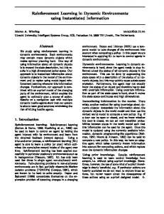
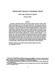
The game environment is shown in figure 1. The red rectangular block is the player. The green rectangular blocks are the platforms on which the player can jump. Let’s call the bottommost platform P1, the middle platform P2, and the topmost platform P3. G refers to the goal point, where the player needs to reach to end the game. P2 is a moving platform. The figure 1a shows the player at the start state and figure 1d shows the player at the goal state (figure 1b and 1c show intermediate player positions).
(a)
(b)
target L’ and his distance from L’ is distL’. Now, the reward provided by the game is a function of action A, L, L’, distL and distL’. If an agent chooses such an action which results in its change of local target and brings him closer to the global target state, i.e., L < L’, the game gives a +400 reward. However, if the new local target is away from the previous target, i.e., L’ < L, the agent will get -400. The L < L’ means the agent is now closer to its global goal. If the local target does not change, i.e., L==L’, and the local target is not 2, i.e., platform 2, then the reward is the difference in the distances, (distL-distL’) – Penalty of action A. The difference in distL and distL’ ensures that moving closer to the local target gives a positive reward and moving farther gives a negative reward. A penalty is also associated with keeping the same local target even after an action. This penalty is action dependent where 0.5 for stay action and 5 for other actions. The stay action is given a less penalty because stay action contributes less in score calculation as shown in equation 2. The lesser the score, the better, thus the game gives priority to stay action by giving it less penalty than others. In case if L==L’==2, the game does not include the difference in the distance while giving the reward. The reason being 2 is a moving platform. Thus, the distance changes irrespective of what action the agent takes. Reward (A, L, L’, distL, distL’) 1. if(L==L’=2) 3.
Reward = Penalty(A)
4. else if (L==L’) 5. (c) (d) Fig. 1. The Jumper Game, where the player is in red color. (a) Shows the initial position of the player and the platforms P1, P2, P3 and the goal state G. (b) Shows the player waiting for moving platform, P2. (c) Shows the player on moving platform, P2. (d) Shows the goal or the final state G of the player.
During the gameplay, the agent has two targets; one is the global target, i.e., the goal state, and the other is the local target, i.e., the intermediate next platform to reach the goal state. There are four local targets, first three being the platforms and the last one being the final goal. A local target for a player can be any value from 1, 2, 3, 4, where the higher local target means closer to the goal. Precisely speaking, the local target 1 is at P1, 2 is at P2, 3 is at P3, and 4 is at G. For example, in figure 1a, the agent first should reach the platform P1 to reach its ultimate target G so; its local target is 1. Similarly, in figure 1b, the new local target for an agent is 2, and in figure 1c, the new local target for an agent is 3. In figure 1d, to reach the goal state, the local target of the agent is 4 which is same as its global target. For each action, the game provides a reward. Consider the player wishes to take an action A. Before taking action, let his local target was L, and his distance from L was distL. As the player has taken action A, it may or may not have changed his local target. The local target changes if the player jumps on a platform from the ground, or jumps on a new platform or jumps to the ground from a platform. Let’s call his new local
Reward = (distL – distL’) – Penalty(A)
6. else if (L < L’) 7.
Reward = +400
8. else (L > L’) 9.
Reward = -400
Penalty (A) 1. if (A=stay) 3.
Penalty = 0.5
4. if (A€{left, right, jumpl, jumpr}) 5.
Penalty = 5
The jumper game has been implemented in two versions: Slow and Fast. During the slow jumper game, the moving platform P2 moves 1 pixel per frame. However, for fast jumper game, the moving platform P2 moves 4 pixels per frame. Total 15 rounds of the jumper game were played, first 5 being the slow rounds and last 10 being fast. The action vector for a round i is defined as:
Action Vector = [N(left), N(right), N(jumpl), N(jumpr), N(stay)] � ����
where N(A) means the count of action A from start to goal state. Action Vector is needed to calculate the score and Mean Squared Deviation. The score for a round is calculated as: Score = N(left)� N(right)�� N(jumpl)�� N(jumpr)������� N(stay)� ����
The lesser the score, the better the performance. The human players and different models were made to play the jumper game. To evaluate the performance of models against human players, we choose Mean Squared Deviation (MSD) as a performance measure. MSD is the average squared difference between human actions and model actions. The MSDAll (over all the rounds) is calculated for the Action Vector (Equation 1) with respect to humans over all the cycles as
�
�
����
Where MSDAll, M is mean squared deviation over all the rounds of model M. AVM, i is the action vector of model M at i th round and AVH, i is the action vector of human player at ith round. Furthermore, we calculated MSD separately for slow and fast rounds given as
�
�
�
�
KEY ACTION MAPPING Action
Left Arrow
left
Right Arrow
right
Up Arrow
jumpr
jumpl
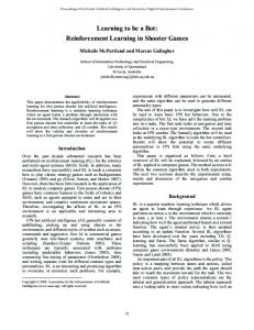
The players were only informed that they had to use these four keys without telling the mapping to actions. If they were inactive for more than 20 frames, it was counted as a stay. Each participant first played 5 rounds of a slow game, then advanced to the faster game in which the platform moved at a 4x speed. For each round, the total number of actions and scores were recorded in a file Also, for each action taken by participants, the experience tuple was also stored in the file for an elaborate record. A state was defined as a vector [X, Y, dis1, dis2, dis3], where X, Y referred to the X, Y coordinates of the player, dis1 was the distance from the platform P1, dis2 was the distance from the platform P2, and dis3 was the distance from the platform P3. B. Results Figure 2 presents the number of actions and score for each round averaged over all the participants. Initially, due to lack of experience, the score is high. However, the score starts decreasing till round five. It further increases in the 6th round due to transition from the slower version of the game to the faster version of the game. After that, the score starts decreasing again as the players adapt themselves to the changed environment.
�
�������������
����
����
����
�
�������������
����
����
A. Experimental Setup Participants could either choose no action for the game or could press one of the arrow keys. The keys were mapped to the actions as shown in Table II. TABLE II.
Down Arrow �
����
IV. HUMAN DATA Fifteen participants in the age group of 20-22 years (Average = 21.07 years and standard deviation = 0.58 years) participated in the jumper game. All the participants were males. They were from an engineering background, studying Computer Science and Engineering, Mechanical Engineering or Electrical Engineering.
Key
�
Fig. 2. The performance of humans in the Jumper game. The x-axis denotes the round number. Y-axis denotes the score or number of actions (left, right, jumpl, jumpr) taken to reach the goal state. The First five cycles are for the slow game, and the last ten cycles are for the fast game.
V. MODELS Three models were selected to play the jumper game. These models are imitation learning, Q learning, and DeepQ network (DQN) model. A. Imitation Learning In a state, the model calculates Euclidean distance between the model state and the human states using the human stateaction pairs. If the distance is less than a pre-defined threshold, then that state is called the relevant state. Next, the probability of each action in the model state is calculated. Each relevant state has an action mapped to it. Say the x number of relevant states have an action left. Then the probability of choosing a
left action is given by P(left) = x/(total number of relevant states). Similarly, probability for other actions is calculated. The action is taken based on the probabilities calculated as mentioned above. The imitation learning algorithm was made to play the jumper game for 15 rounds. Model played first 5 rounds of slow games followed by 10 rounds of fast games. Ten simulated players participated in the jumper game. B. Q Learning Q-Learning [6] is a type of model-free reinforcement learning algorithm. The objective of this algorithm is to select optimal actions for a given Markov Decision process. Q learning algorithm maintains a Q-table that consists of states and actions. It calculates the rewards associated with each action in a state. Initially, all the rewards are instantiated as zero. The Q-table gets updated using the following Bellman equation (see equation 6 below). The Q value of an action At in a state St is determined by equation 6:
�
� ����
Where, QSt,At is the Q value for a given state St and an action At at time t. The rt is the reward observed on taking action At. The ��is the learning rate, and γ is the discount factor. The discount factor allows us to decide how important the possible future rewards are compared to the present reward. For a given state St at time t, the action with highest Q value is most suitable. For the jumper game, the set of actions includes At ϵ�{left, , right, jumpl, jumpr}, the learning parameter ( ���is set to 0.01, and the discount factor (γ) is set to 0.85. For exploration in the jumper game, we use another parameter, i.e., the probability e. The value of e is set to be high (0.15) for initial rounds and low (0.03) for later rounds for both slow and fast variants of the jumper game (these values were obtained using trial-and-error). Thus, for a state St at time t, we choose a completely random action with the probability e or the action with highest Q value with probability (1-e). The jumper game was divided into 33 states, and a state structure was maintained as coordinate
C. DeepQ Network Deep Q Network (DQN) [4] is a first deep reinforcement learning algorithm to demonstrate how an AI agent can learn to play games by just observing the screen without any prior information about those games. In DQN algorithm, a neural network is used to approximate the reward based on the state. The model agent should be able to process game’s screen output. The use of convolutional network helps to consider the image regions instead of independent pixels. Unlike the statebased algorithms, where the states should be initialized at proper places, here we just provide the images of the jumper game to the algorithm. The implementation was done in python using Tensor Flow library [29]. 1) Preprocessing and Model Architecture Working with the raw frames of the jumper game, which was 800 x 600 pixels image, can be computationally complex. So, we applied basic preprocessing and compressed the pixels to a lower pixel size (84, 84, 3). DQN model uses four convolutional layers, which downsamples the data. This down-sampling is followed by one fully connected layer. We downsample the data using strides and “VALID” padding. � Figure 3 shows the architecture of our DQN with different assumptions. The blocks indicate the feature maps; the arrows in between them indicate the weights. The compressed image was passed through the four convolutional layers as shown in the figure. The output of the convolutional layers is flattened to an array of dimension 512*1 which is then split into advantage and value feeds [13]. The feeds are added to get the Q values. Let Q(s, a) be the Q value of an action a, in the state S. It can be broken into value and advantage. Value, i.e., V(s) is the measure of how good a particular state is, Advantage, i.e., A(s, a) tells how good a particular action a is in given state s. Q(s,a) = A(s,a) + V(s)
Dis1, Dis2, Dis, Q-Value of Actions = {‘left’:v1, ‘right’:v2, ‘jumpl’:v3, ‘jumpr’:v4,”stay”:v5}. Here, are the state’s coordinates.
Dis1 refers to the distance from platform P1, Dis2 from platform P2 and Dis3 from platform P3. When the player is in a state, the most similar state (out of the 33 initialized) is retrieved using similarity. The similarity is calculated based on the Euclidean distance between the player’s coordinates and state’s coordinates. The lesser is the distance, the more the similarity. If more than one state is fetched, then we use second similarity method. Let the distance of player from platform P1 be dis1’, from P2 be dis2’ and from P3 be dis3’. Euclidean distance between the distance of retrieved states from platform and the distance between player from platform


![[PDF] Better Business Decisions Using Cost Modeling - Google Sites](https://m.moam.info/img/260x300/pdf-better-business-decisions-using-cost-modeling-_6478a83a097c4744708d13bd.jpg)