Proceedings of the 40th IEEE Conference on Decision and Control Orlando, Florida USA, December 2001
FrP11-1
Modeling flow statistics using the linearized Navier-Stokes equations1 Mihailo Jovanovi´ c
Bassam Bamieh
[email protected]
[email protected]
Department of Mechanical and Environmental Engineering University of California, Santa Barbara, CA 93106-5070
Abstract
currently possible.
We develop a model for second order statistics of turbulent channel flow using an associated linear stochastically forced input-output system. The correlation operator of the velocity fields is computed by solving the appropriate Lyapunov equations of a Galerkin approximation of the original system. We use a variety of excitation force correlations and show the dependence of the velocity fields statistics on them. By using certain excitation correlations, we are able to closely match flow statistics computed from Direct Numerical Simulation (DNS) of channel flow. The implications of these result for the proper weight selection in optimal control problems for channel flow are discussed.
In this paper, we address the problem of modeling disturbances in the LNS equations by testing the validity of a stochastically excited version of this model. The LNS equations are considered with stochastic body forcing as an input, and we investigate the correlation operator of the various velocity fields for a variety of input correlation models. We compare the results of this analysis with correlation data from DNS of the full Navier-Stokes equations in turbulent channel flow. Our basic computational tool is a matrix approximation of the operator Lyapunov equation for the velocity field covariance. This approximation is obtained using a Galerkin scheme. The paper is organized as follow: In Section 2, we give a detailed description of the LNS equations with body force inputs and present them as an evolution equation for an infinite dimensional system. In Sections 3 and 4, we give a brief summary of the theory of linear infinite dimensional systems with stochastic inputs, and show how the covariance operator can be used to compute various flow statistics such as the Reynolds stresses. Our numerical results are summarized in Section 5, where we show how DNS correlations can be matched by the present model with an appropriate selection of input forcing covariance. We end in section 6 with some conclusions regarding the validity of the LNS equations with input as a control-oriented model for turbulent channel flow.
1 Introduction There has been much recent interest in the problem of turbulence suppression in channel flow using active feedback control of boundary conditions. This problem is viewed as a benchmark problem for turbulence control in a variety of geometries, including boundary layers. There has also been mounting evidence [1, 2, 3, 4, 5, 6, 7] that the linearized NavierStokes (LNS) equations provide an accurate model of the dynamics of transition, and of the dynamics of the near wall layer in fully turbulent boundary layers. The key observation is that in shear flows, one must include either signal or model uncertainty in the LNS equations since they are extremely sensitive to perturbations. These facts have motivated several researchers [8, 9] to use the LNS equations for model based controller design for channel flows. Furthermore, the above mentioned results imply that the proper turbulence suppression controller design paradigm is that of disturbance attenuation or robust stabilization rather than pole placement. Successful schemes based on LQG (H2 ) and H∞ have been used to design linear controllers for nonlinear channel flow dynamics in DNS simulations [10, 11]. One of the important open questions remaining is the type of disturbance models to include in the problem set-up. This is of course equivalent to the question of weight selection for the corresponding optimal or robust control design problem. As is well known, proper weight selection can dramatically alter control performance when the controller is in feedback with the actual nonlinear system. It is therefore anticipated that proper weight selection can lead to successful turbulence suppression with linear controllers at higher Reynolds numbers than
2 Navier-Stokes Equations The flow of an incompressible viscous Newtonian fluid can be described by the nonlinear NS equations and the continuity equation 1 (1a) ∂t u = − ∇u u − ∇p + ν∆u, ρ 0 = ∇ · u, (1b) where u is the velocity vector, p is pressure, ρ is fluid density, and ν is kinematic viscosity. ∇ is the gradient, ∆ := ∇2 is the Laplacian, and the operator ∇u is given by ∇u := u · ∇. We shall proceed by linearizing (1a) around a chosen steady state nominal flow condition (¯ u, p¯). If we decompose the instantaneous fields into the sum of the nominal profiles and the deviations from them, i.e. ¯ +u ˜ , p := p¯ + p˜, then we can rewrite (1a) as u := u ˜ ∂t u
1 Research
supported in part by a DOD MURI grant for ”uncertainty management in complex systems”.
0-7803-7061-9/01/$10.00 © 2001 IEEE
4944
=
1 ˜ − ∇u˜ u ¯ − ∇˜ − ∇u¯ u p + ν∆˜ u ρ ½ ¾ 1 ¯ − ∇¯ ˜. + ν∆¯ u − ∇u¯ u p − ∇u˜ u ρ
(2)
The linearized Navier-Stokes equations are obtained by ˜ . If the linearizaneglecting the second order term ∇u˜ u tion of (1a) is done around a laminar flow condition the expression between the curly brackets on the righthand side of (2) is zero. We will however, consider the ¯ is not laminar. more general situation when u
By exploiting spatial invariance in the streamwise and spanwise directions, (5) can be parametrized by the spatial frequencies kx and kz and rewritten as a onedimensional PDE in the wall normal direction
In [7] externally forced incompressible NS equations linearized around laminar flow profile have been considered. In this paper we analyze a more general setting in which nominal flow condition is allowed to be nonlaminar 1 ˜ = −∇u¯ u ˜ − ∇u˜ u ¯ − ∇˜ p + ν∆˜ u + d, ∂t u ρ ˜, 0 = ∇·u
where the operators Aˆ and Bˆ represent Fourier transforms of their counterparts on the right-hand side of (5). Further, it can be shown that the original streamwise and spanwise velocity perturbations can be extracted as functions of vˆ, ω ˆ y , kx and kz
∂t ψˆ
where d can account for flow disturbances, surface irregularities, neglected nonlinearities or the non-laminarity ¯. of u
=
The inner product on the right hand side of equation (10) is the standard inner product on L2 [−1, 1] defined by (12). This inner product is chosen as it has a physical significance. Namely, it yields a norm on the state space which measures kinetic energy density of a harmonic perturbation, which is defined for any given pairs of spatial frequencies in the streamwise and spanwise directions and at any given time as Z Z Z kx kz 1 2π/kx 2π/kz 2 E := (u + v 2 + w2 ) dz dx dy. 16π 2 −1 0 0 E can be expressed as a quadratic form of vˆ and ω ˆy using integration by parts and (9) Z 1 D E ˆ Qψˆ . E = (12) ψˆ∗ Qψˆ dy =: ψ, −1
and B :=
·
S
:=
−U ∂x + ν∆,
:=
−U 0 ∂z ,
∆−1 0
3 Stochastically Excited LNS Equations In this section a brief summary of the theory of linear infinite dimensional systems with stochastic inputs is given. Interested reader is referred to [6] and references contained therein for more details.
¡ ¢ ∆−1 −U ∂x ∆ + U 00 ∂x + ν∆2 ,
C
0 I
¸·
2 − ∂xy ∂z
A system (8) subject to stochastic external excitation with know second-order statistics is considered. If dˆ is a temporally stationary white process with zero mean, then its covariance operator is given by ˆ 1 )dˆ∗ (t2 )} = Rδ(t ˆ 1 , t2 ) := E{d(t ˆ 1 − t2 ), where R ˆ is R(t the ‘spatial’ correlation operator. By further assuming that the generator of the dynamics Aˆ is stable, the steady-state limit of the correlation operator of ψˆ
(6)
2 2 ∂xx + ∂zz 0
2 − ∂yz − ∂x
(9)
where Q is a block diagonal linear operator given by · ¸ 1 −∆ 0 Q := . (11) 0 I 8(kx2 + kz2 )
Evolution form model of the linearized NS equations subject to external forces was derived in [7] and has the following form: · ¸ · ¸· ¸ v L 0 v = + Bd ∂t ωy C S ωy (5) =: Aψ + Bd, :=
=
e
Since the fluctuation velocity field has to satisfy the continuity equation it follows that the entire state of system (3) can be parameterized using only two fields. A particularly well-suited parameterization is given in terms of the wall normal velocity and vorticity fields as follows ¸ · ¸ · u 0 I 0 v v . (4) = ψ := ∂z 0 −∂x ωy w
L
w ˆ
i (kx ∂y vˆ − kz ω ˆy ) , kx2 + kz2 i (kz ∂y vˆ + kx ω ˆy ) . kx2 + kz2
(8)
We endow the state space with an inner product of the form D E E D ψˆ1 , ψˆ2 (10) := ψˆ1 , Qψˆ2 ,
1 − ∂x p + ν∆u + du , ρ 1 ∂t v + U ∂x v = − ∂y p + ν∆v + dv , (3) ρ 1 ∂t w + U ∂x w = − ∂z p + ν∆w + dw . ρ £ ¤∗ ¤∗ £ ˜ := u v w , d := d u dv dw where u , 0 and U := ∂y U . An appropriate definition of d can be used to recover linearized version of (2) from (3). This fact would often be exploited in the remainder of our paper.
where
=
ˆ Aˆψˆ + Bˆd,
We stress that the evolution model has the same form regardless of whether the linearization is performed around laminar or any flow condi£ other steady ¤state ∗ ¯ = U (y) 0 0 tion, as long as u and p¯ = p¯(x), 2 2 because ∂xy {ν∂yy U − ρ1 ∂x p¯} = 0. This fact is often used in our analysis.
Let us assume that the only nonzero component of the steady state velocity field is velocity in £ the streamwise ¤∗ £ ¤∗ ¯ := U V W = U (y) 0 0 direction, u and that the nominal pressure depends only on the ¯− streamwise coordinate, p¯ = p¯(x). Then, ν∆¯ u − ∇u¯ u ¤∗ £ 2 1 1 U − ∂ p ¯ 0 0 ν∂ ∇¯ p becomes equal to and x yy ρ ρ one can rewrite the forced linearized NS equations as ∂t u + U ∂x u + U 0 v
u ˆ
=
¸ . (7)
4945
ˆ ˆ ˆ := limt→∞ V(t) := limt→∞ E{ψ(t) (V ψˆ∗ (t)}), can be determined as a solution of the operator algebraic Lyapunov equation ˆ + V ˆ Aˆ∗ = − M, ˆ Aˆ V
ˆ x , y1 , y2 , kz ) is the kernel representation of where V(k ˆ It can be shown that the kernel repthe operator V. resentation of the 3D operator V, whose action is described by1
(13) g(x1 , y1 , z1 ) = R +1 R R V(x1 − x2 , y1 , y2 , z1 − z2 )f (x2 , y2 , z2 )dz2 dx2 dy2 −1 R R
ˆ := Bˆ R ˆ Bˆ∗ . Note that the operators Aˆ∗ and where M ˆ respectively. Bˆ∗ represent adjoint operators of Aˆ and B, ˆ on a Hilbert space with The adjoint of an operator H an inner product h·, ·ie , is defined by D
ˆ ψˆ2 ψˆ1 , H
E
D e
=
ˆ ∗ ψˆ1 , ψˆ2 H
ˆ by a Fourier transform is related to the kernel of V Z Z ˆ x , y1 , y2 , kz ) = V(k V(x, y1 , y2 , z)e−i(xkx +zkz ) dxdz.
E e
,
R
(14) Therefore
which must hold for all ψˆ1 , ψˆ2 in the Hilbert space. Aˆ∗ can be determined using (14), while the adjoint of the operator Bˆ is given by D E D E ˆ Bˆdˆ ˆ dˆ , ψ, = Bˆ∗ ψ, (15)
V(x, y1 , y2 , z) =: lim E {ψ(¯ x, y1 , z¯, t) ψ ∗ (¯ x + x, y2 , z¯ + z, t)} t→∞ Z Z ˆ x , y1 , y2 , kz )ei(xkx +zkz ) dkx dkz , = V(k R
e
n o ˆ x , y1 , kz , t) ψˆ∗ (kx , y2 , kz , t) . ˆ x , y1 , y2 , kz ) := lim E ψ(k V(k t→∞
Since the generator Aˆ is a 2 × 2 lower block triangular operator, we can equivalently rewrite (13) as the set of conveniently coupled equations of the form [6]
Let us now express the wall normal velocity and vorticity fields in terms of particular vˆ and ω ˆ y basis functions φn (y) and ψn (y)
ˆ11 + V ˆ11 Lˆ∗ = −M ˆ 11 , LˆV (16a) ∗ ˆ ˆ ˆ ˆ ˆ ˆ ˆ S V21 + V21 L = −(M21 + C V11 ), (16b) ∗ ˆ22 + V ˆ22 Sˆ∗ = −(M ˆ 22 + CˆV ˆ21 ˆ21 Cˆ∗ ). (16c) SˆV +V
vˆ(kx , y, kz , t) = ω ˆ y (kx , y, kz , t) =
ˆ 21 M ˆ 22 M
=
∗ ∗ ˆ 22 Bˆ12 ˆ ∗23 Bˆ12 Bˆ12 R + Bˆ13 R + ∗ ∗ ˆ ˆ ˆ ˆ ˆ ˆ B12 R23 B13 + B13 R33 B13 , ∗ ∗ ˆ 12 Bˆ12 ˆ 13 Bˆ13 Bˆ21 R + Bˆ21 R ,
(17b)
=
∗ ˆ 11 Bˆ21 Bˆ21 R .
(17c)
∞ X
an (kx , kz , t)φn (y),
(18)
bn (kx , kz , t)ψn (y),
(19)
n=0 ∞ X n=0
In the important special case of 3D streamwise constant perturbations, the Orr-Sommerfeld and Squire operators become self-adjoint [6], (Lˆ∗ = Lˆ = ν∆−1 ∆2 , 2 Sˆ∗ = Sˆ = ν∆ = ν(∂yy − kz2 I)), and the adjoint of the coupling operator is given by Cˆ∗ = −ikz ∆−1 U 0 . ˆ can be Furthermore, the elements of the operator M expressed as =
R
where
where the inner product on the right hand side of (15) is assumed to be the standard L2 [−1, 1] inner product.
ˆ 11 M
R
These are to be chosen so that the boundary conditions on vˆ and ω ˆ y are satisfied (see [7] for details). In equations (18,19), an (kx , kz , t) and bn (kx , kz , t) represent so-called spectral coefficients. With a slight abuse of notation, we refer to them as an (t) and bn (t), bearing in mind that they are functions of time parametrized by spatial frequencies kx and kz . By applying the Galerkin procedure to equation (8) we obtain an infinite dimensional ODE for the spectral coefficients an and bn , parametrized by spatial frequencies kx and kz . If we solve the operator algebraic Lyapunov equation for thus obtained system we will get a representation ˆ kernel in the chosen basis. This opof the operator V’s erator is an infinite matrix for any given pair (kx , kz ) ˆb (kx , kz ). We also rewrite vˆ and it will be denoted by V and ω ˆ y as
(17a)
System of equations (16) is used in Section 5 for numerical computations of the steady-state statistics of 3D streamwise constant velocity perturbations.
vˆ
4 Steady State Statistics of the Velocity Field In this section we show how the steady state correlaˆ can be used to compute the Reynolds tion operator V ˜ ∗ }, for the case when the flow stresses, τ r := −ρE {˜ uu is driven by external excitation with known statistics and is assumed to satisfy the linearized NS equations. It is important to notice that, for every pair of spatial ˆ represents an operator from frequencies kx and kz , V L2 [−1, 1] to L2 [−1, 1]. This means that for any given ˆ x , kz )fˆ is to be computed fˆ, gˆ ∈ L2 [−1, 1], gˆ = V(k as Z +1 ˆ x , y1 , y2 , kz )fˆ(kx , y2 , kz ) dy2 , gˆ(kx , y1 , kz ) = V(k
ω ˆy
= =
∞ X n=0 ∞ X
an (t)φn (y) =: φ∗ (y)a(t),
(20)
bn (t)ψn (y) =: ψ ∗ (y)b(t),
(21)
n=0
where φ(y) and ψ(y) (a(t) and b(t)) represent column vectors with an infinite number of elements for any given y (any given triple (kx , kz , t)). Taking this into account, the state of (8) takes the following form · ¸ · ∗ ¸· ¸ vˆ φ (y) 0∗ a(t) ψˆ := = , (22) ω ˆy 0∗ ψ ∗ (y) b(t) 1 Spatial invariance in the x and z directions has been exploited in the definition of operator V.
−1
4946
where 0 represents an infinite column vector with all elements equal to zero (0∗ is an infinite zero row vector). We are now able to write the definition of the operator ˆb (kx , kz ) in terms of a and b V ¾ ½· ¸ ¤ a(t) £ ∗ ˆb (kx , kz ) := lim E a (t) b∗ (t) V . b(t) t→∞
20
18
16
14
U
12
8
6
4
2
0 −1
ˆ ˜ is given Based on (9), the operator that maps ψˆ into u by ikx ∂y −ikz I 1 ˆ 2 2 ˆ (23) ˆ ψ. ˆ ˜ = 2 0 u (kx + kz )I ψ =: K kx + kz2 ikz ∂y ikx I (−ikz ψ ∗ )(y) · ¸ a 0 b (ikx ψ ∗ )(y) (24) Thus, the kernel representation of the velocity fluctuations correlation operator in the frequency domain can be expressed as ˆ x , y1 , y2 , kz ) := P(k n o ˆ ˆ ˜ (kx , y1 , kz , t) u ˜ ∗ (kx , y2 , kz , t) = lim E u t→∞ ½ · ∗ ¸· ¸ φ (y1 ) 0∗ a ˆ lim E K 0∗ ψ ∗ (y1 ) b t→∞ · ¸¾ ¤ £ ∗ 0 ˆ ∗ φ(y2 ) a b∗ K = 0 ψ(y2 ) · ∗ · ¸ ¸ 0∗ 1) ˆ φ (y ˆb (kx , kz )K ˆ ∗ φ(y2 ) 0 K V ∗ ∗ 0 ψ(y2 ) 0 ψ (y1 ) Therefore, the steady state value of Reynolds stress is ˆ x , y1 , y2 , kz ) in the following manner related to P(k :=
˜ ∗ (x, y2 , z, t)} −ρ lim E {˜ u(x, y1 , z, t) u t→∞ Z Z ˆ x , y1 , y2 , kz )ei(xkx +zkz ) dkx dkz , −ρ P(k
=
R
−0.6
−0.4
−0.2
0 y
0.2
0.4
0.6
0.8
1
All simulations are done at kx = 0, which means that the one point correlations in the streamwise direction have been computed. The spanwise direction is ‘covered’ by 256 grid points, and vˆ and ω ˆ y are approximated by a linear combination of 50 basis functions. The mean velocity profile shown in Figure 1 is approximated by a polynomial. Then, the matrix representations of the underlying operators in the evolution model (obtained by linearization around this polynomial) are determined using a numerical scheme that we developed. Selected steady-state statistics of the 3D velocity field perturbations for the case of a spatially uncorrelated ˆ = I, at Rτ = 180 are shown external excitation, R in Figure 2. These plots illustrate one point correlations in the three spatial directions. In other words, selected Reynolds stress components are computed in terms of the operator V evaluated at x = z = 0 and y1 = y2 =: y, i.e. V(0, y, y, 0). The solid line represents results obtained by solving (16), while the dashed line represents results obtained by DNS of the fully developed turbulent channel flow [12, 13]. All statistics are scaled such that their maximal value is equal to one. Clearly, there are almost no similarities between our results and those obtained in [12, 13]. In the remainder of this section, we try to explain why such a large discrepancy occurs. We also illustrate that considerably better results can be achieved by considering the entire problem from a more general point of view.
(25)
R
1
1
0.8
0.8
0.6
0.6
u
rms
which represents a 3×3 symmetric matrix for any given quadruple (x, y1 , y2 , z).
vrms
lim τ r (x, y1 , y2 , z)
−0.8
Figure 1: Turbulent mean velocity profile at Rτ = 180.
Combining (22) and (23) yields (ikx ∂y φ∗ )(y) 1 2 2 ∗ ˆ ˜= 2 u ((kx + kz )φ )(y) kx + kz2 ∗ (ikz ∂y φ )(y)
t→∞
10
0.4
0.4
0.2
Considerations contained in this section represent a theoretical foundation that is used for numerical computation of the steady-state velocity field statistics.
0.2
0 −1
0 −0.5
0 y
0.5
1
−1
5 Numerical Results
−uvbar
rms
w
0.5
1
−0.5
0 y
0.5
1
0.5
0.6 0.4
0
−0.5
0.2 0 −1
0 y
1
1 0.8
This section contains an analysis of the results obtained by computing the steady-state statistics of the velocity field which is assumed to satisfy NS equations linearized around a turbulent mean velocity profile. This velocity profile is shown in Figure 1, and it was obtained by DNS of the channel flow at Rτ = 180 [12, 13].
−0.5
−1 −0.5
0 y
0.5
1
−1
Figure 2: Selected scaled steady-state statistics of the turbulent channel flow (dashed) and the linearized ˆ = I at Rτ = 180. NS equations (solid) for R
A numerical scheme for employing finite dimensional representations of the operators in (8) is described in detail in [7]. This scheme is developed in Matlabr , and it exploits the spatial invariance of the equations in the x and z directions. The PDE in the remaining wallnormal direction was approximated numerically using the Galerkin method.
Recent work [14] has indicated that turbulence statistics can be better matched with a stochastically forced linear system model if one uses finite rather infinite time correlations. Finite time correlations are com-
4947
puted by accumulating the variance over times no longer than a ‘coherence time’ Tc . This has been accomplished by simply setting the velocity field to zero for all time instants larger than Tc . We point out that an intuitively equivalent model is derived by introducing an ‘exponential discounting’ in the state of the linearized model, ψ1 (t) := e−αt ψ(t), α > 0. These exponentially discounted correlations are derived from the solution of the following Lyapunov equation: ˆ Bˆ∗ . ˆ + V ˆ (Aˆ − αI)∗ = − Bˆ R (Aˆ − αI) V
1
0.8
R22y
0.6
0.4
0.2
0 −1
−0.5
0.5 1 y
−1
y2
1
ˆ 22y as a function of y1 and y2 . Figure 3: R
dashed curves in the regions close to the walls. Furthermore, one can notice an almost perfect match between the vrms that we computed and the one obtained from DNS. Deviations in wrms can be explained by the fact that we have not even attempted to choose forcing statistics that would decrease them. Our objective was to illustrate that by changing statistics of the excitation, we can considerably influence the shape of velocity field statistics, a point proven by our computations. Certainly, there is significant room for improvement of the obtained results and investigations along these lines are a topic of ongoing research. 1
0.8
0.6
0.6
v
rms
Let us consider equation (16a) and try to adjust the ˆ11 with desired propˆ 11 in order to obtain V operator M erties. It can be shown that both vrms and wrms at ˆ11 . Our kx = 0 can be determined based on only V objective is to accomplish a close correspondence between vrms and its DNS counterpart, if possible. Based ˆ 11 depends on R ˆ 22 , R ˆ 23 , and on (17a), notice that M ˆ R33 , which illustrates that choosing the forcing statistics is a nontrivial problem. Because of that, we asˆ 33 = 0 and channel our efforts on ˆ 23 = R sume R ˆ 22 . Once we adjust R ˆ 22 , we can comchoosing R ˆ pute M11 and then (16a) can be used for obtaining ˆ 23 and R ˆ 33 . We propose operator expressions for R ˆ 22 to be a stationary white process in t, x and z, R ˆ 22 := E{dv d∗v } = R ˆ 22y δ(t1 − t2 )δ(x1 − x2 )δ(z1 − z2 ), R ˆ with R22y defined as a sum of rank-one operators
1
0.8
wrms
A question of interest is whether one can model statistics of the external excitation such that the results obtained by solving system (16) represent a good enough approximation of those reported in [12, 13]. In order to address this important issue, observe that our results fail to match the DNS-based ones in the vicinity of the walls. We can argue that it is hardly plausible from a physical perspective to expect the same forcing intensity near the walls and in the middle of the channel. This might be a reasonable explanation of the mismatch between solid and dashed curves in Figure 2.
N X
0
0
According to our numerical investigations, in the simplest possible scenario of a spatially uncorrelated external excitation, neither of these techniques leads to a significant improvement compared to the infinite temporal correlations.
ˆ 22y = R ˆ 22y (y1 , y2 ) := R
1 0.5
−0.5
0.4
0.4
0.2
0.2
0
−1
0
−0.5
0 y
0.5
1
−1
−0.5
0 y
0.5
1
Figure 4: Selected scaled steady-state statistics of the turbulent channel flow (dashed) and the linearized ˆ 22y shown in Figure 3 NS equations (solid) for R at Rτ = 180.
The values of −uv and urms can be computed using the solutions of equations (16b) and (16c), respectively. Note that these solutions do not influence vrms and wrms because of the one-way coupling in system (16). A question that we face again is how to determine statistics of forcing that yields satisfactory correlations. ˆ 21 Namely, at this stage we have to specify operators M ˆ 22 in order to compute V ˆ21 and V ˆ22 . If we asand M ˆ 12 = R ˆ 13 = 0 and R ˆ 11 = I, a considerable sume R mismatch will still be present. For that reason, we ˆ 21 and M ˆ 22 equal to zero and resort set operators M to some kind of ‘exponential discounting’ in the process of solving (16b,16c) by replacing operator Sˆ by Sˆ − αI. It is important to stress that even though we originally thought of using this transformation based on a finite time correlations approach [14], what we are doing cannot be interpreted as ‘discounting’, since, as can be readily shown, it is not possible to obtain a time invariant Lyapunov equation without introducing ‘discounting’ in both states. However, it turns out that for α = 1, results obtained using this procedure match their DNS counterparts surprisingly well, as illustrated in Figure 5. More importantly, an interestˆ 21 and M ˆ 22 can ing interpretation of the operators M now be made. In particular, they can be computed in terms of solutions of ‘discounted’ system (16b,16c) ˆ 21 = −αV ˆ21 and M ˆ 22 = −2αV ˆ22 . Furthermore, as M
fn (y1 )fn∗ (y2 ).
n=1
Functions fn are to be chosen such that they have a large value near one wall, a small value in the vicinity of the other wall, and belong to some intermediate range in between. Note that N determines the rank of the ˆ 22y . In particular, for N = 2 with operator R ½ gn (y), 0.5 ≤ |y| ≤ 1, fn (y) := gn (y) + 1.6(0.1 − 0.4y 2 ), |y| ≤ 0.5. n 2 ˆ 22y is a where gn (y) := e−3.1(y+(−1) 0.9) , n = 1, 2, R band limited operator, as illustrated in Figure 3. ˆ 22y , (16a) is solved for For the above defined operator R ˆ V11 and the solution value is used for computation of vrms and wrms . Figure 4 shows a comparison between scaled DNS results and results obtained using our procedure. Clearly, the chosen statistics of external excitation provide very good agreement between solid and
4948
ˆ can be the corresponding elements of the operator R ˆ 21 and determined using the above expressions for M ˆ 22 , the definition of the operator B, ˆ and equations M (17b,17c). It is important to notice that these elements ˆ 12 , R ˆ 13 and R ˆ 11 ) are no longer stationary in the (R spanwise direction, which is an important, hitherto unknown feature. It is interesting that the nonzero values ˆ 12 & R ˆ 13 ) of the of the cross-correlation operators (R external excitations play a prominent role.
References [1] L. H. Gustavsson, “Energy Growth of ThreeDimensional Disturbances in Plane Poiseuille Flow,” J. Fluid Mech., vol. 98, p. 149, 1991. [2] K. M. Butler and B. F. Farrell, “ThreeDimensional Optimal Perturbations in Viscous Shear Flow,” Physics of Fluids A, vol. 4, p. 1637, 1992. [3] S. C. Reddy and D. S. Henningson, “Energy Growth in Viscous Channel Flows,” J. Fluid Mech., vol. 252, pp. 209–238, 1993. [4] B. F. Farrell and P. J. Ioannou, “Stochastic Forcing of the Linearized Navier-Stokes Equations,” Physics of Fluids A, vol. 5, no. 11, pp. 2600–2609, 1993. [5] L. N. Trefethen, A. E. Trefethen, S. C. Reddy, and T. A. Driscoll, “Hydrodynamic Stability Without Eigenvalues,” Science, vol. 261, pp. 578–584, 30, July 1993. [6] B. Bamieh and M. Dahleh, “Energy Amplification in Channel Flows with Stochastic Excitation,” submitted to Physics of Fluids, CCEC report 98-1012, University of California at Santa Barbara, http://www.engineering.ucsb.edu/∼bamieh, 1998. [7] M. R. Jovanovi´c and B. Bamieh, “The SpatioTemporal Impulse Response of the Linearized NavierStokes Equations,” in Proceedings of the 2001 American Control Conference, pp. 1948–1953, 2001. [8] L. Cortelezzi, K. H. Lee, J. Kim, and J. Speyer, “Skin-Friction Drag Reduction Via Robust ReducedOrder Linear Feedback Control,” International Journal of Computational Fluid Dynamics, vol. 11, no. 1-2, pp. 79–92, 1998. [9] T. R. Bewley and S. Liu, “Optimal and Robust Control and Estimation of Linear Paths to Transition,” Journal Fluid Mechanics, vol. 365, pp. 305–349, 1998. [10] M. H¨ ogberg and T. R. Bewley, “Spatially localized convolution kernels for decentralized control and estimation of transition in plane channel flow,” Submitted to Automatica, 2000. [11] K. H. Lee, L. Cortelezzi, J. Kim, and J. Speyer, “Application of robust reduced-order controller to turbulent flows for drag reduction,” Physics of Fluids, vol. 13, no. 5, pp. 1321–1330, 2000. [12] J. Kim, P. Moin, and R. Moser, “Turbulence Statistics in Fully Developed Channel Flow at Low Reynolds Number,” J. Fluid Mech., vol. 177, pp. 133– 166, 1987. [13] T. R. Bewley, P. Moin, and R. Temam, “DNSBased Predictive Control of Turbulence: an Optimal Benchmark for Feedback Algorithms,” submitted to J. Fluid Mech., 2000. [14] B. F. Farrell and P. J. Ioannou, “Perturbation Structure and Spectra in Turbulent Channel Flow,” Theoret. Comput. Fluid Dynamics, vol. 11, pp. 237– 250, 1998. [15] M. R. Jovanovi´c and B. Bamieh, “Input-Output Properties of the Linearized Navier-Stokes Equations,” in preparation, 2001.
1 1 0.8 0.6
0.8
0.4 0.2
−uv
urms
bar
0.6
0.4
0
−0.2 −0.4
0.2
−0.6 −0.8
0 −1 −1
−0.5
0 y
0.5
1
−1
−0.5
0 y
0.5
1
Figure 5: Selected scaled steady-state statistics of the turbulent channel flow (dashed) and the linearized NS equations (solid) obtained as a solution of (16b,16c) for Sˆ → Sˆ − αI at Rτ = 180.
The results of this section have shown that we have ˆ that been able to specify elements of the operator R provide a close correspondence between our results and those that are considered to be a benchmark. Our current efforts are directed towards development of a precise methodology which would determine external excitation statistics that would guarantee matching DNS-based data in some optimal (e.g. least-squared) sense [15]. 6 Concluding Remarks This paper has dealt with the input-output analysis of the externally excited linearized NS equations when the input is assumed to be a stochastic field with given second order statistics. The statistics of the resulting random velocity field are related to the input statistics through the system dynamics, and can be computed by solving Lyapunov equations. We have shown that when the input excitation is assumed to be spatially and temporally white, the resulting velocity field statistics are significantly different from DNS data. There are many possibilities for adjusting the input excitation statistics, so that the resulting velocity field statistics in the LNS equations match those from DNS data. We presented one such set of input correlations. These input correlations with the LNS equations are therefore an accurate statistical model for real turbulent channel flow (i.e. DNS results). It is natural to propose the use of these input correlations as a disturbance model in an LQG control problem for channel flow. It is expected that an LQG controller thus designed would have superior performance than a controller designed without an accurate disturbance model.
Acknowledgments The authors would like to thank Tom Bewley for providing DNS data of the statistics of turbulent channel flow.
4949