This paper deals with modeling heat transport through phonon conduction in bulk and ... upto order n in the external perturbation is sufficient to determine the energy ... scattering is the so-called boundary scattering, where the phonon mean free .... calculations require switching representations from real to reciprocal space ...
MODELING HEAT CONDUCTION FROM FIRST-PRINCIPLES Keivan Esfarjani*, Jivtesh Garg# and Gang Chen+ *
Department of Mechanical and Aerospace Engineering and Institute of Advanced Materials, Devices and Nanotechnology, Rutgers University, Piscataway, NJ 08854, USA # Department of Aerospace and Mechanical Engineering, University of Oklahoma, Norman, OK 73019, USA +
Department of Mechanical Engineering, MIT, Cambridge, MA 02139, USA Recent progress in computer architecture and electronic structure calculation methods based on density functional theory (DFT) have made the computation of thermal transport properties of crystalline solids possible and accurate. In this article we review the most recently developed methodologies applied to modeling the phonon thermal conductivity from first-principles DFT methods. Most of the emphasis will be on the intrinsic three-phonon processes. Modeling of impurity and boundary scattering processes will also be described. Finally applications to simple bulk materials, superlattices and alloys will be presented to illustrate the power and accuracy of the approach.
1
NOMENCLATURE 𝛼, 𝛽, 𝛾 … Cartesian coordinates 𝒃 basis atom 𝒌, 𝒒 wavevectors in the first Brillouin Zone 𝑮, 𝑹 reciprocal and direct translation lattice vectors 𝑚, 𝑀 (kg) atomic mass and mass matrix 𝑘 = (𝒌 𝜆) general phonon mode 𝜆 phonon branch Λ (m) phonon mean free path 𝜔 (1/cm) phonon frequency 𝜎 (1/cm) phonon self-energy 𝜏 (s) phonon relaxation time 𝑣 (m/s) phonon 𝑘 group velocity 𝛾𝒌! , 𝛾! mode Gruneisen parameter 𝐶! , 𝐶𝒌! (J/K) heat capacity per mode 𝐶!!! 𝑎𝑛𝑑 𝑀!!! (1/s) collision and modified-collision matrix elements 𝐽! (Jm/s2) 𝛼-component of the heat current density 𝜅!" (W/mK) thermal conductivity tensor ! 𝑛!" , 𝑛!" Non-equilibrium and equilibrium phonon disribution function (a.k.a occupation numbers) 𝛿𝑛! , 𝜙! deviation and rescaled deviation from equilibrium distribution 𝜗!"# 𝑟 (V) electronic external potential 𝜓(𝑟) electronic eigenfunction 𝐺! 𝜔 = 𝐺! ′ + 𝑖𝐺! " (cm2) unperturbed phonon Green’s function 𝐷 𝜔 (States /s m3) phonon density of states 𝑃, 𝜋 (kg m/s, m kg1/2/s) cartesian and rescaled atomic momentum !" 𝑃!!! Probability of coalescence per unit time 𝑆 symmetry operation 𝑇 (K) Temperature 𝑇!! ! , 𝑇!! ! (eV/Ang2, eV/kg/Ang2 ) T and rescaled T matrix elements 𝑢, 𝑤 (m,m kg1/2) cartesian and rescaled atomic displacement 𝑤!→!! (1/s) relaxation rate from state k to k’ Φ (eV/Ang2) harmonic force constants Ψ (eV/Ang3) anharmonic force constants BA Born approximation DFT density functional theory DFPT density functional perturbation theory FP first-principles FBZ first Brillouin zone FGR Fermi golden rule MFP mean free path (N)EMD (non-)equilibrium molecular dynamics RTA relaxation time approximation SMRT single mode relaxation time
1 INTRODUCTION This paper deals with modeling heat transport through phonon conduction in bulk and nanostructured crystals using first-principles methods. Such methodology could be free of any fitting parameter, and if the model is appropriately chosen, it can have good 2
prediction capability. From our experience on modeling several semiconductor materials, we have observed that the deviations of the predicted thermal conductivity from experimental data are typically on the order of 10% and usually less than 20%. This error depends on the choice of the interaction model for which we have some freedom. There is always a tradeoff between accuracy and computational cost. The most sophisticated modeling of thermal transport in solids through conduction has been done in the past based on the solution of the Boltzmann equation within the relaxation time approximation (RTA)[1], [2]. In such atomistic description of insulators or semiconductors heat is transported by phonons, which are the quanta of vibrations in solids1. The latter are calculated either using the Debye and Einstein models, or using a force field-model combined with the lattice dynamics theory. The parameters of the force field are usually fitted to reproduce the available experimental data on the elastic properties or phonon frequencies. Such approach often gives agreement in phonon dispersion with experimental data to within 10-20%. Prediction of the phonon lifetimes, however, is not very accurate because the latter depends on the third derivatives of the potential and the force field parameters are usually not fitted to reproduce correct third derivatives. So there is no reason why phonon lifetimes should come out to be accurate using this approach. This is why we will be using accurate first-principles method to extract the second, and more importantly, the third derivatives of the potential energy in order to produce accurate phonon lifetimes. Other approaches to calculate the bulk thermal conductivity also exist. They include equilibrium molecular dynamics (EMD) and the use of the Green-Kubo formula[3], [4] to get the thermal conductivity from the heat current autocorrelations[5]. Non-equilibrium molecular dynamics (NEMD) is another path where a temperature difference is imposed on the system and the heat flux measured[6],[7] Both these methods are classical and cannot predict thermal conductivity at low temperatures. They also suffer from errors due to statistical averaging, and could be very time-consuming due to size scaling issues. In what follows, we will focus on the methodology based on the solution to the Boltzmann transport equation for phonons in a crystal, as we believe this approach, in addition to its higher accuracy, gives us access to more detailed information, namely the relaxation time and mean-free path (MFP) of all phonon modes. This information is crucial in understanding and controlling transport of heat in crystalline materials. Accurate estimate of second-order and third-order derivatives, needed for prediction of thermal conductivity, was made possible by the development of density-functional perturbation theory (DFPT)[8–10]. DFPT is a linear response theory and relies upon the use of “2n+1” theorem which states that the knowledge of the electronic wave-function upto order n in the external perturbation is sufficient to determine the energy derivatives with respect to the strength of the derivative upto order 2n+1. Giannozzi et al. [11] used the density functional perturbation theory to compute the second order interatomic force constants and lattice dynamical properties of Si and Ge and obtained excellent agreement between computed and measured phonon dispersions. This demonstrated the accuracy of second order force constants obtained through DFPT. 1
In metals, most of the heat is carried by electrons. In this chapter, however, we will be interested only in the phonon contribution to the thermal conductivity, which is dominant in semiconductors and insulators.
3
To compute thermal conductivity a knowledge of phonon lifetimes is also required. The first truly ab initio calculation of the linewidth (inverse of phonon lifetime) of a phonon mode at the Γ point was performed by Debernardi et al [8] who obtained third-order interatomic force constants by extending the DFPT using the “2n+1” theorem[12]. By using the lowest order three-phonon processes Debernardi et al obtained excellent agreement between the calculated and experimental Raman linewidths for Si and Ge upto temperatures well above the room temperature. Similar results for Raman linewidth were subsequently obtained by Lang et al[13]. These results proved the accuracy of third-order interatomic force constants derived through DFPT. For the calculation of thermal conductivity knowledge of just the phonon linewidth at Γ is insufficient. Phonon relaxation times of thousands of wave-vectors in the entire Brillouin zone are needed to compute thermal conductivity. This was first accomplished by Deinzer et al who derived both the second and third order derivatives using DFPT and used them to compute the phonon linewidth of arbitrary wave-vector [14]. Another approach to estimate the third order interatomic force constants based on use of supercells was implemented by Esfarjani et al [15]. Estimate of thermal conductivity requires Boltzmann transport equation to be solved for the unknown perturbed phonon populations. An exact solution of the linearized Boltzmann transport equation based on the three-phonon processes was first obtained by Omini and Sparavigna [16] using an iterative process. Broido et al. [17] combined the force constants derived from DFPT along with such an exact solution of the Boltzmann transport equation to predict thermal conductivity of Si and Ge in a fully ab initio way and obtained excellent agreement between theory and experiment. This approach was subsequently applied to diamond[18] and several compound semiconductors[19] with good success. A variational approach to solve the phonon Boltzmann[20] was also recently implemented. Garg et al. used the first-principles approach to study alloys [21] as well as superlatttices[22]. Esfarjani et al. [15] developed a real-space supercell approach to estimate the third order interatomic force constants and used these to compute the thermal conductivity of silicon [23], followed by half heuslers[24], PbTe[25] and GaAs[26]. Below we describe some of these approaches in more detail.
2 BOLTZMANN-PEIRELS THEORY OF THERMAL TRANSPORT The relaxation time comes from a combination of several phonon scattering processes present in the system. For small size or nanostructured systems, one major source of scattering is the so-called boundary scattering, where the phonon mean free path (MFP) is limited by the dimensions of the nanostructures. The MFP is the average distance travelled by a phonon of given frequency, before it undergoes a scattering. It is related to the phonon relaxation time by: Λ 𝜔 = 𝑣 𝜔 𝜏 𝜔 .Boundary scattering is the dominant process at low temperatures even in bulk materials[27], [28] because at low frequencies anharmonic and impurity scattering rates (in 𝜔! and 𝜔! respectively) are negligible compared to the boundary scarttering rate which is on the order of 𝑣/𝐿 and thus finite. 4
The other source of phonon scattering is defects or impurities, which can also be extended to alloys and solid solutions. This process is dominant at intermediate temperatures smaller than the Debye temperature, where there are not too many phonons present. For low-frequency, long wavelength phonons, the impurity scattering rate is proportional to the fourth power of the phonon frequency. This is the well-known Rayleigh scattering limit. Finally at higher temperatures, near and above the Debye temperature, where the phonon concentration is large, three or more phonon scattering processes dominate transport. They result from the anharmonicity of the force constants, meaning that terms in the force which are quadratic or of higher power in atomic displacements cause the multi-phonon scattering processes. When all processes are present and compete, the combination rule that gives the total relaxation time is given by the following equation sometimes referred to as the Matthiessen’s rule: ! ! ! ! =! +! +! ( 2-1) ! boundary
defect
!"#!$%&"'(
This rule basically states that the rates of different independent processes add to give the total scattering rate2. The phonon or lattice thermal conductivity is then given by the RTA to the solution of Boltzmann equation[29]: ! ! 𝜅 = !! ! !" 𝜏!" 𝑣!" 𝐶!" ( 2-2) !
!!
where the heat capacity per phonon mode is defined as 𝐶!" = ℏ𝜔!" !"!" , 𝜏!" and 𝑣!" are respectively the relaxation time and group velocity of the mode 𝑘𝜆, 𝑁! is the number ofconsidered modes in the summation, Ω is the volume of the unit cell, and the factor of 3 in the denominator is used to get the isotropic thermal conductivity in 3 dimensions. More details about the derivation of this formula and its more general form are given in the appendix.
2.1 Boundary scattering processes As mentioned, this term dominates thermal conductivity at low temperatures because the corresponding rate is constant[30]. The MFP is on the order of the sample size for a monocrystalline sample, but for a nanostructured or grannular material, the largest MFP is typically on the order of grain or nanostructure dimensions. The assumption here is that at the interface there is a high probability of reflection and most phonons do not pass through the domains unscattered. So domain size limits the MFP of phonons. More accurate ways to compute the MFP of all phonons in a nanostructured system would be to use the Monte Carlo techniques[31],[32] or solving the Boltzmann equation using interface scattering as boundary conditions[33]. For this purpose, one needs to know the relaxation time of the phonon due to impurity and 3-phonon processes. At the surface or interface one also needs to make assumptions about the scattering probability in different directions. Such input can be provided from accurate transmission/reflection calculations using Green’s functions method[34] or molecular dynamics simulations [35]. Given all 2
The above expression treats boundary scattering on equal footing as internal scattering, while a more rigorous approach is to treat the boundary scattering as interface conditions in solving the Boltzmann equation. This approach was adopted by Fuchs[36] and Sondheimer[37] who found the analytical solution to Boltzmann transport equation in a thin film.
5
the possible scattering probabilities, one can follow the trajectory of a phonon mode and deduce its MFP by performing an average over the unscattered paths of all generated phonons with different initial positions and momenta. !
!"#$%&'( In the case of a dirty interface, the formula 1/𝜏!" = !!" where L is the grain size is often used. Variations on this formula include multiplication by the “specularity” term (1 + 𝑝)/(1 − 𝑝) for a nanowire or thin film which models surface roughness[1]. The parameter p is called the specularity or the “polish of the surface” parameter and varies between 0 for perfectly rough and 1 for perfectly “smooth” surface where there is specular reflection. Ziman[1] has also developed a wavelength-dependent model for p. This simple formula, unfortunately can not distinguish between a nanowire of diameter L or a thin film of thickness L or a polycrystal of average grain size L. A more accurate treatment of boundary scattering in the case of a nanowire and thin film was done by Fuchs[36] and Sondheimer[37] who independently solved the Boltzmann equation in a thin film geometry including the surface scattering as a boundary condition. In the thick sample limit (Λ ≪ L) it was found that the conductivity was reduced, relative to its bulk ! !!! !! value, by a factor 1 + !" ! where P is the perimeter and S the cross-section of the cylinder which can be of any arbitrary shape. In the very thin limit (Λ ≫ L) , the !!! ! reduction is !!! ! implying that other than for the specularity factor, the mean free path
of the bulk is replaced by an effective MFP which is the sample thickness. This, to some !"#$%&'( extent, justifies the replacement 𝜏!" by 𝐿/𝑣!" . In a “kinetic theory” approach, Chambers[38] introduced a position and momentumdependent distribution function from which an effective size and position-dependent MFP maybe deduced[39], [40]. Using this type of approach has also shown some success, but, to our knowledge, still required some fitting[41].
2.2 Impurity scattering processes The rate for this process is known to be in 𝜔! at low frequencies, and was first derived by Lord Kelvin (Rayleigh). A more general derivation based on perturbation theory (Born approximation) was provided by Tamura[42]. This calculation produces a rate ! proportional to 𝜔! valid at low frequencies: !(!) ∝ 𝛿𝑚 𝑚 ! 𝜔! 𝐷(𝜔) where 𝐷(𝜔)is
the phonon density of states proportional to 𝜔! at low frequencies (in 3D), leading to the well-known Rayleigh law. One shortcoming of the Born approximation is that it cannot differentiate between heavy and light masses, because it is proportional to the square of 𝛿𝑚 𝑚. Full calculations of the scattering rates, however, produce different results especially at higher frequencies and mass contrast. Therefore the corresponding rates might differ at high temperatures. These calculations are based on the T-matrix formalism, and can be done once the harmonic phonon Green’s function is known[43]. The perturbation parameter is either the mass mismatch or the force constant mismatch between the impurity and the host. For the case of Ge in bulk Si for instance, 𝛿𝑚/𝑚 ≈ 1.6 and it is therefore a large parameter. The Born approximation is not expected to be accurate in this case. Another physical phenomenon that might occur and which cannot be predicted using Born approximation is the resonance scattering effect: If the 6
frequency of the incident phonon matches or is close enough to that of a localized impurity mode, resonance occurs. Mathematically, this can be seen as the pole of the phonon Green’s function. This resonance scattering will produce a large peak in the phonon scattering cross section at that frequency. The T-matrix approach is the exact method which can handle impurity scattering. In what follows, we will describe how this method can be used to exactly calculate elastic scattering rates due to impurities or defects. Formally, if the unperturbed force constant matrix is shown by 𝛷! , and the local perturbation by 𝛿𝛷 , then the T-matrix is defined as: 𝑇 = 𝛿𝛷 + 𝛿𝛷 𝐺! 𝛿𝛷 + ⋯ = 1 − 𝛿𝛷 𝐺! !! 𝛿𝛷; 𝐺! being the unperturbed retarded Green’s function defined by: 𝐺! (𝜔) = 𝑀𝜔! − 𝛷! + 𝑖𝜂 !! Here 𝑀 is the mass matrix and 𝜂 is an infinitesimal positive number enforcing causality as a boundary condition[34], [44]. One has the possibility of changing representation and use √𝑚 𝑢 as the new dynamical variables. In this case, the force constant matrix will be renormalized by the mass and one may define the renormalized Green’s function as !! 𝐺! (𝜔) = 𝜔! − 𝛷! + 𝑖𝜂 with 𝑀!!/! 𝛷! 𝑀!!/! = 𝛷! . The above definition of the Tmatrix still applies for the renormalized GF and perturbation 𝛿𝛷 , i.e. 𝑇 = 1 − !!
𝛿𝛷 𝐺! 𝛿𝛷 . The impurity scattering rate for phonons is given by Fermi’s Golden rule (FGR): !
!
! 𝑤!→!! = ! 𝑇!!! 𝛿(𝜔!! − 𝜔!! )
(2-3)
!
where the matrix elements of the 𝑇 matrix are computed in the momentum representation, although for the initial evaluation of the T-matrix it is more efficient to calculate !! 𝑇 = 1 − 𝛿𝛷 𝐺! 𝛿𝛷 in real space since the perturbation 𝛿𝛷 is localized . These calculations require switching representations from real to reciprocal space as the Green’s function 𝐺! is easily evaluated in the momentum space. The matrix for this basis change is the unitary matrix 𝑒 !𝒌.𝑹 times the normal modes basis, eigenvectors of the dynamical matrix, to be described in section 5 below. To get the lowest-order Born limit, one simply needs to substitute 𝑇 by 𝛿𝛷. To obtain the total scattering rate, one needs to sum over all final momenta: ! !!
=
!! 𝑤!→!!
=−
! !" !!! !!
( 2-4)
!!
where the second equation is obtained using the optical theorem. If needed, the scattering cross section 𝜎 is always related to the rate by: 1 = 𝜏! 𝑣! 𝜎! 𝑛 = 𝛬! 𝜎! 𝑛 where 𝑣! is the phonon velocity, and n is the impurity concentration. This equation basically states that if there are n scattering centers per unit volume, on the average a single scattering event happens in the volume determined by 𝛬! 𝜎! corresponding to one impurity, which takes the volume 1/n. This is because 𝛬! is the average distance travelled by the phonon of mode k between two successive collisions, and 𝜎! is the effective cross-section pertaining to a single scatterer. As a simple illustration, we can consider scattering by an impurity of strength V, localized on one atomic site only. In this case, the total scattering cross section is proportional to:
7
𝜎 ∝ −𝑉 𝐺! " / 1 − 𝑉𝐺!
!
= −𝑉𝐺! "/[ 1 − 𝑉𝐺!!
!
!
+ 𝑉𝐺!" ]
( 2-5)
where only the diagonal element (i,i) of the unperturbed Green’s function needs to be calculated and 𝐺! = 𝐺!! + 𝑖 𝐺!" was used. As already mentioned, this is done using the spectral representation: 𝐺! iα, jβ, ω! =
!
∫
!! ! !!
!
! ! 𝒊 𝒒! ∗ ! ! 𝒋 𝒒! ! !!" ! ! !!!"
( 2-6)
! The phonon eigenvalues 𝜔!" and eigenvectors 𝑒 ! 𝒊 𝒒𝜆 will be defined in the following section on lattice dynamics (see Eq. 3-5). A “resonance” condition maybe obtained by investigating the case where the real part of the denominator in the cross section becomes zero. In the simple case of a localized impurity, where V is a constant, this results in 𝐺!! 𝑖, 𝑖, 𝜔! = 1/𝑉 and the cross section ! ! becomes 𝜎 = !" ! ∝ !"# ! . This implies scattering resonance is largest at the band !
edges where the phonon density of states goes to zero. One can still have the real part of the denominator be zero as the resonance condition, but if this happens at the middle of the band, resonance would be weak or unobservable depending on the DOS value at that frequency. In other words, for a resonance scattering to be observable, the strength of the impurity scattering needs to be such that the frequency at which 𝐺! ′ 𝑖, 𝑖, 𝜔! = 1/𝑉 occurs, has to be near the band edge.
2.3 Three-phonon anharmonic processes At higher temperatures where phonons abound, the anharmonic processes dominate phonon transport, meaning the multi-phonon scattering processes occur much more often than boundary or defect scattering. Furthermore, this is an intrinsic scattering property of the material which does not depend on its size and shape and doping or defect structure3. The dominant process, which usually provides a good approximation to the thermal conductivity is the 3-phonon process. Although higher order processes also exist, their rate is usually lower than 3 phonon until the temperature is raised to a very high value. For this reason, we will only be concerned with the lowest-order (3-phonon) processes. This assumption will be validated when we will compare our theoretical findings with experimental results. The basis for the computation of the corresponding scattering rates is the lattice dynamics theory which we will explain below.
3 LATTICE DYNAMICS REVIEW Lattice Dynamics (LD) is a well-known and well-developed theory which has been studied in many references[45], [46]. For the sake of completeness, we will briefly describe it in this section. In this theory, the lattice potential energy is written as a Taylor expansion of the atomic displacements about the equilibrium positions. Keeping up to the second order terms in the potential energy is called the harmonic approximation. In this limit the model can be solved analytically after going to the normal mode representation. This theory has the advantage of becoming exact at low temperatures where atomic displacements have small amplitude. 3
As long as doping and size effects do not alter the phonon dispersion, we assume that the multiphonon scattering rates are independent of the doping and system size.
8
! !𝑹𝒃
H!"#$%&'( =
𝑹𝒃 !!𝒃
+
! 𝑹𝑹! 𝒃𝒃! !
!
! Φ!" 𝑹𝒃, 𝑹! 𝒃! 𝑢𝑹𝒃 𝑢𝑹! 𝒃!
( 3-1)
Here α,β are the Cartesian directions (x,y,z), R is a lattice translation vector and b represents a basis atom within the unit cell. To calculate the phonon lifetimes, we will only keep the third-order terms in the expansion, and will use perturbation theory. The same formalism will be used to calculate the scattering rates, which will involve very similar expressions. The scattering rates will be used if one wants to solve the Boltzmann equation beyond the relaxation time approximation. H!"#$! =
! 𝑹𝑹! 𝑹!! 𝒃𝒃! 𝒃!! !!
!
!
! Ψ!"# 𝑹𝒃, 𝑹′ 𝒃′ , 𝑹′′ 𝒃′′ 𝑢𝑹𝒃 𝑢𝑹! 𝒃! 𝑢𝑹!! 𝒃!!
( 3-2)
Before we start to solve the harmonic Hamiltonian, let us go over the symmetry properties of the force constants as these relations need to be enforced for a set of FCs to be physically correct.
3.1 Symmetries of the force constants: The following symmetry relations must be satisfied by all the force constants: -Symmetry under permutation of the indices. This is due to the fact that force constants are high-order derivatives of the crystal potential energy, and as such should not change under permutation of the order of derivation. 𝜕!𝐸 ! ! Φ!" 𝑹𝒃, 𝑹 𝒃 = = Φ!" 𝑹! 𝒃! , 𝑹𝒃 ! ! 𝜕𝑢𝑹𝒃 𝜕𝑢𝑹! 𝒃! Likewise we should have: Ψ!"# 𝑹𝒃, 𝑹! 𝒃! , 𝑹!! 𝒃!! = Ψ!"# (𝑹!! 𝒃!! , 𝑹𝒃, 𝑹! 𝒃! ) = Ψ!"# (𝑹! 𝒃! , 𝑹!! 𝒃!! , 𝑹𝒃) -Translational invariance. This symmetry requires the total potential energy or forces not to change if the system (all atoms) is shifted by an arbitrary constant vector. It is also referred to as the acoustic sum rule (ASR). Φ!" 𝑹𝒃, 𝑹! 𝒃! = 0 ; ∀(𝛼𝛽𝑹! 𝒃! ) 𝑹𝒃
Ψ!"# 𝑹𝒃, 𝑹! 𝒃! , 𝑹!! 𝒃!! = 0 ; ∀(𝛼𝛽𝛾 𝑹! 𝒃! 𝑹!! 𝒃!! ) 𝑹𝒃
-Discrete translational invariance. In addition, in a crystal, force constants between a pair and their translation by a crystal lattice vector should be the same. Φ!" 𝑹𝒃, 𝑹! 𝒃! = Φ!" 𝟎𝒃, 𝑹! − 𝑹 𝒃! ; ∀(𝛼𝛽 𝑹𝒃 𝑹! 𝒃! ) Ψ!"# 𝑹𝒃, 𝑹! 𝒃! , 𝑹!! 𝒃!! = Ψ!"# 𝟎𝒃, 𝑹! − 𝑹 𝒃! , 𝑹!! − 𝑹 𝒃!! -Rotational invariance. This symmetry requires the total potential energy or forces not to ! change if all atoms are rotated by an arbitrary angle about an arbitrary direction. If 𝜫𝟎𝒃 is the 𝛽 component of the first derivative of the potential energy with respect to basis atom 𝒃, and 𝜖 !"# is the antisymmetric Levy-Civita symbol, then we must have: 9
!
Φ!" 𝟎𝒃, 𝑹! 𝒃! (𝑹! +𝒃! )! 𝜖 !"# + 𝜫𝟎𝒃 𝜖 !"# = 0 ; ∀(𝛼𝜈𝒃) !
!𝑹! 𝒃!
Ψ!"# 𝟎𝒃, 𝑹! 𝒃! , 𝑹!! 𝒃!! (𝑹!! +𝒃!! )! 𝜖 !"# + 𝚽!" 𝟎𝒃, 𝑹! 𝒃! 𝜖 !"# !"𝑹!! 𝒃!!
+ 𝚽!" 𝟎𝒃, 𝑹! 𝒃! 𝜖 !"# = 0 ; ∀(𝛼𝛽𝜈𝒃𝑹! 𝒃! ) As can be seen, rotational invariance constraints relate force constants of a given rank to those of a lower rank, implying that they cannot be chosen arbitrarily. -Huang invariance. This symmetry expresses the invariance of the elastic constants tensor if the Voigt indices are switched. It would trivially be satisfied for a bravais lattice or a high symmetry unitcell, but if needs to be separately enforced if the primitive cell has many atoms and is of low symmetry. Basically if under external stress atoms in the primitive cell do not relax according to the strain tensor, this constraint needs to be imposed. -Group symmetry. Besides the invariance under translations by a lattice vector, each crystal has inherent symmetry operations such as rotations and mirror planes, leaving it invariant. If these operations are represented by a matrix S, we should have: Φ!" 𝑹𝒃, 𝑹! 𝒃! = Φ!" 𝟎𝒃, 𝑹! − 𝑹 𝒃! Φ!" 𝟎𝒃, 𝑹! 𝒃! = !!!! 𝑆!!! 𝑆!!! Φ!! !! (𝑆 !! 𝟎𝒃 , 𝑆 !! 𝑹! 𝒃! ) Ψ!"# (𝟎𝒃, 𝑹! 𝒃! , 𝑹!! 𝒃!! ) = !! !! ! ! !! !! !! ! ! ! ! ! ! 𝑆!! ! 𝑆!! ! 𝑆!! ! Ψ!! !! !! (𝑆 (𝟎𝒃), 𝑆 (𝑹 𝒃 ), 𝑆 (𝑹 𝒃 )) In order for a force constant model to be physically correct, all the above symmetries need to be enforced. This is a necessary requirement as, in practice, we use a finite size supercell, and cut the range of force constants off beyond some range. Although the raw force constants will not satisfy all these relations, we need to modify them in accordance with these symmetries/constraints. This was done in reference [15] using a singular value decomposition, as the calculated force-displacement data from FP-DFT and the symmetry constraints are both linear in the force constants. It was observed that the violation of the invariance relations, following this procedure, was usually several (4 to 6) orders of magnitude smaller than the typical scale of the FCs as long as the chosen cutoff range was reasonable. Another possible way to “clean up” the force constants i.e. imposing the invariance constraints after the FCs are calculated, is via the Lagrange multiplier method as proposed by Mingo et al[47].
3.2 Normal modes and Harmonic theory We start by calculating the harmonic normal modes in a crystal. The normal (Bloch) modes and the conjugate momenta P are defined as: ! 𝑢𝒒𝒃 =
1 𝑁
! ! 𝑢𝑹𝒃 𝑒 !𝒒.𝑹 ; 𝑢𝑹𝒃 =
𝑹
10
1 𝑁
! 𝑢𝒒𝒃 𝑒 !!𝒒.𝑹
𝒒
! 𝑃𝒒𝒃 =
1 𝑁
! ! 𝑃𝑹𝒃 𝑒 !!𝒒.𝑹 ; 𝑃𝑹𝒃 =
𝑹
1 𝑁
! 𝑃𝒒𝒃 𝑒 !𝒒.𝑹
𝒒
Using this transformation, it is possible to decouple the harmonically interacting atoms into N independent oscillators, one for each 𝒒. The sum over 𝒒 is extended to the firstBrillouin zone (FBZ) since these expressions are manifestly invariant under 𝒒 → 𝒒 + 𝑮, where 𝑮 is a reciprocal lattice vector satisfying 𝑮𝒊 . 𝑹𝒋 = 2 𝜋𝛿!" ;(i,j=1,2,3). N is the number of 𝑹 -vectors or 𝒒 -points which is “infinity.” In the normal mode representation, the harmonic Hamiltonian becomes: H!"#$%&'( =
𝒒
!
!𝒒! !!𝒒! !!!
!
+!
𝒃𝒃! D!"
!
! 𝒃𝒃! 𝒒 𝑢𝒒𝒃 𝑢!𝒒𝒃!
( 3-3)
where the dynamical matrix is defined as D!" 𝒃𝒃′ 𝒒 = 𝑹 Φ!" 𝟎𝒃, 𝑹𝒃! 𝑒 !𝒒.𝑹 , and use was made of translational invariance of the force constants. If atomic masses within the primitive unit cell are different, a further change of variable 𝑤!" = 𝑚! 𝑢!" allows the elimination of the mass variables in the kinetic energy term and a renormalization of the dynamical matrix. Finally, diagonalizing the massrenormalized dynamical matrix, results in a fully diagonalized Hamiltonian in which the internal modes 𝒃, 𝒃! are decoupled as well: H!"#$%&'( = where 𝜋𝒒! =
𝒒!
!𝒒! !!𝒒! !
!!𝒒.𝑹 ! ! ! 𝑹𝒃! 𝑃𝑹𝒃 𝑁! 𝑒 !
!
! + ! 𝜔𝒒! 𝑤𝒒! 𝑤!𝒒!
𝑏 −𝒒𝜆 and 𝑤𝒒! =
( 3-4) ! 𝑹𝒃! 𝑢𝑹𝒃
!! !
𝑒 !𝒒.𝑹 𝑒 ! 𝑏 𝒒𝜆
Here 𝑒 ! 𝑏 𝒒𝜆 are the eigenvectors of the mass-renormalized dynamical matrix, satisfying: 𝒃!!
!!" 𝒃𝒃! 𝒒 !𝒃 !𝒃!
! 𝑒 ! 𝒃′ 𝒒𝜆 = 𝜔𝒒! 𝑒 ! 𝒃 𝒒𝜆
( 3-5)
They also satisfy conjugation, orthonormality and completeness relations: 𝑒 ! 𝒃 −𝒒𝜆 = 𝑒 ! 𝒃 𝒒𝜆 ∗ ; 𝑒
!
𝑒 ! 𝒃 𝒒𝜆 𝑒 ! 𝒃 𝒒! 𝜆! = 𝛿!!! 𝛿!𝒒𝒒! !𝒃 !
𝒃 𝒒𝜆 𝑒
𝒃′ −𝒒𝜆 = 𝛿!" 𝛿𝒃𝒃!
!
Note that there are as many normal modes 𝜆 as there are degrees of freedom within the primitive unit cell (the number of possible pairs 𝛼𝒃). The eigenmodes or normal modes are also referred to as “phonons”. In a semiclassical picture, they are thought of as free “particles” with a momentum 𝒒. Acoustic phonons having a linear dispersion do not have a mass, while optical phonons do. Thinking of a phonon of given momentum be in a certain location requires the consideration of a wavepacket i.e. a superposition of several
11
normal modes. In this way, it is possible to have a “quasiparticle” with given position and momentum with still some uncertainty satisfying the Heisenberg uncertainty principle.
4 PHONON FREQUENCY SHIFTS AND LIFETIMES Within the harmonic approximation the phonons (normal modes) have infinite lifetime. Including higher-order terms in the Taylor expansion of the potential energy will create scattering terms reducing the lifetimes to a finite value. These perturbations will in principle also have the effect of shifting the phonon frequencies. The phonon lifetimes due to cubic anharmonic interactions can be found using second-order perturbation theory. Alternatively, using many-body theory, one can compute the self-energy associated with this perturbation[45],[48]. The latter case provides a more general and systematic description of the effect of perturbations on an exactly solvable Hamiltonian: the self-energy is a complex number, the real part of which describes the frequency shift and its imaginary part provides the inverse lifetime of the phonons: 𝑖 𝜎 𝑞𝜆, 𝜔 = 𝛥 𝑞𝜆, 𝜔 − 2 𝜏 𝑞𝜆, 𝜔 These terms can be more or less accurately calculated depending on what perturbations are considered and to what order. In the above relation the frequency 𝜔 is not the phonon frequency but the one at which the response is being calculated. The shifted frequency is obtained via the solution of 𝜔 = 𝜔!" + 𝛥 𝑞𝜆, 𝜔 , but in practice, to lowest order, one just substitutes the “on-shell” frequency to get the renormalized phonon frequency: 𝜔!"#$!%&'()!" = 𝜔!" + 𝛥 𝑞𝜆, 𝜔!" and 𝜏 𝑞𝜆) = 𝜏(𝑞𝜆, 𝜔!" The expression for the phonon self energy is given by[45], [46]: !
𝜎 𝒒𝜆, 𝜔 = − !ℏ!
!",!!±!
𝑉! 1,2, 𝒒𝜆
!
!!! !!!! !! !! !!! !!"!
+!
!!! !!!! ! !!! !!"!
( 4-1)
where the complex frequency is defined as 𝜔! = 𝜔 + 𝑖 0! , 1 and 2 are labels of two phonon modes from arbitrary bands in the FBZ, with 𝑛!! being the corresponding equilibrium phonon occupation number (Bose-Einstein distribution function), and finally the 3-phonon matrix element 𝑉! is given by: 1 ℏ 𝑉! 1,2, 𝒒𝜆 = 𝑁 2
! !
𝛹!! !! !! 𝑹𝟏 𝒃𝟏 , 𝑹𝟐 𝒃𝟐 , 𝑹𝟑 𝒃𝟑 𝑒 ! 𝑹𝒊 𝒃𝒊 !!
×
𝒒𝟏 .𝑹𝟏 !𝒒𝟐 .𝑹𝟐 !𝒒𝟑 .𝑹𝟑
𝑒 !! 𝒃𝟏 1 𝑒 !! 𝒃𝟐 2 𝑒 !! 𝒃𝟑 𝒒𝜆 𝑚!! 𝑚!! 𝑚!! 𝜔! 𝜔! 𝜔!"
Note that due to invariance of the cubic FCs under translations of lattice vectors 𝑹, the above term is zero unless 𝒒𝟏 + 𝒒𝟐 + 𝒒𝟑 = 𝑮. The cubic anharmonic term is responsible for 3-phonon scattering processes, meaning that a given phonon can either be converted to 2 other phonons, or combine with another one to produce a third phonon of higher frequency. The energy conservation can be seen ! ! by using the identity !±!!! = 𝑃 ! ∓ 𝑖𝜋𝛿(𝑥) : in the imaginary part, which represents the inverse lifetime, terms such as 𝛿(𝜔! − 𝜔! ± 𝜔! ) which guarantee energy conservation, will appear. 12
In practice, a small non-zero value for the small imaginary part can be considered, the Dirac delta function is then converted to a Lorentzian, and the integration in the FBZ replaced by a discrete summation. A more accurate alternative would be to perform the integration including the Dirac delta function using the tetrahedron method[49], [50] . The Kramers-Kronig relation may then be used to recover the real part if needed. The latter approach is more accurate as it does not require the introduction of an arbitrary imaginary number and has faster convergence properties compared to a regular 𝒒-mesh summation. Using the invariance of the cubic force constants under lattice translation vectors 𝑹, one can show that the above expression also contains momentum conservation 𝛿𝒒𝟏 !𝒒𝟐 !𝒒,𝑮 , where 𝑮 is a reciprocal lattice vector. In this sum, 𝑮 = 0 terms correspond to the socalled “Normal processes”, while 𝑮 ≠ 0 terms are referred to as “Umklapp processes”. The latter are dominant for higher frequency phonons and cause the thermal resistance as they change the phonon momentum direction. They are essentially effective in relaxing the phonon momentum distribution. Normal processes are usually dominant at lower frequencies and serve to thermalize the phonons. Both processes, since inelastic, contribute to the relaxation of the phonon energy distribution. In fact unlike impurity and boundary scattering, they are the only processes which accomplish energy relaxation. It can be shown that the rate for both processes usually scales as 𝜔! where the integer 𝑛 depends on the lattice symmetry[51]. We showed analytically[23] that in Si crystal normal processes have a rate of 𝜔! , while umklapp processes rate is 𝜔! , therefore as previously mentioned, normal processes dominate at low frequencies while umklapps dominate at higher frequencies.
4.1 The Callaway model of thermal conductivity We should note that in the relaxation time approximation, the time 𝜏 which appears in the thermal conductivity (Eqs. (2-1) and (2-2) ) is replaced by the phonon lifetime, which ! ! ! includes both normal and umklapp with the same weights: !!"# = !! + !! This is not exactly true because this equation incorporates the normal process rate in the thermal resistance. In materials where the normal scattering rate is much larger than umklapp, this model underpredicts the thermal conductivity. To overcome this shortcoming, Callaway developed a simple model[52] to account for this underprediction. This was later improved by Allen[53]. Since Normal processes conserve momentum, they relax the non-equilibrium distribution to a quasi-equilibrium one with the same total momentum. This distribution can be thought of as a shifted Bose-Einstein equilibrium distribution in momentum space: 𝑛∗ (ℏ𝜔) = 𝑛! (ℏ𝜔 − 𝜆. 𝑘) . This is considered as a “shift” because Callaway has implicitly assumed a linear dispersion to ease k-space integrations. In reality a shift should be of the form 𝑛∗ (ℏ𝜔) = 𝑛! (ℏ𝜔 − 𝜆. 𝑣! ) Only umklapp (or momentum non-conserving) processes, can relax the momentum to zero, so that the total rate of relaxation of the non-equilibrium distribution due to collisions is given by: !" !!!∗ !!! = − − !! ! ( 4-2) !" !! !
13
If we denote the “exact” relaxation time which should enter Eq. (2-2)) by 𝜏! , then the non-equilibrium distribution can be written to lowest order in temperature gradient as: !! 𝛿𝑛 = 𝑛 − 𝑛! = −𝜏! 𝑣. 𝛻𝑇 !"! Substitution of this form in the Boltzmann equation with collision term given by Eq. (4-2) relates the exact relaxation time to the normal and umklapp ones through: ! 𝜏! = 𝜏 !"# 1 + !! with 𝛽 𝑣. 𝛻𝑇/𝑇 = −𝜆. 𝑘/ℏ𝜔 The only unknown parameter to be determined is the “drift” vector 𝜆. Callaway finds it by imposing that the rate of change of total phonon momentum due to normal processes is zero, while Allen imposes that the average crystal momentum should be the same as that weighted by the shifted distribution: ! 𝑘 (𝑛! − 𝑛!∗ ) = 0. The two theories provide slightly different results for 𝜆 and the resulting 𝜏! . We refrain from giving explicit formulas and refer the reader to the papers by Callaway[52] and Allen[53]. The latter contains a discussion of the difference in the obtained formulas.
4.2 Phase space effect We can note from Eq. (4-1) that there are two contributions in the lifetimes. One is the phase space, and the other the strength of the anharmonic interactions 𝑉! . While the latter mainly depends on the strength of the third-order force constants, the former depends on the volume in the phase space in which 3-phonon processes satisfying the conservation of energy and momentum can occur. This volume only depends on the phonon dispersion curves, and to characterize it, one can simply compute the “joint density of states” for the mode 𝑞 = (𝒒𝜆), as it contains both constraints of energy and momentum conservation: 1 𝑃± 𝑞 = 𝛿(𝜔! − 𝜔! ± 𝜔!!!!!! ) 𝑁! !,!
It is basically the reproduction of the imaginary part of Eq. (4-1) where the phonon occupations reflecting temperature effects and the anharmonicity reflected by 𝑉! are set to 1. 𝑃± tells us basically in how many ways can the phonon mode 𝑞 = (𝒒𝜆) possibly participate in a 3-phonon process. The overall volume can be obtained by summing the above term over all modes 𝑞 . This is a good metric, when comparing thermal conductivities of different materials, of how important is the phase space compared to the strength of anharmonicity (measured by mode Gruneisen parameters). We will now proceed to the first-principles methodologies to calculate harmonic and anharmonic force constants. Knowledge of second and third order force constants allows computation of all relevant parameters needed for thermal conductivity calculation within the lattice dynamics-Boltzman transport equation formalism.
5 DENSITY-FUNCTIONAL PERTURBATION THEORY This method is based on the linear response theory[9], and provides an exact formula for the calculation of the potential energy derivatives with respect to the Fourier transform of ! the atomic displacements 𝑢𝒒𝒃 . The Hellman-Feynman theorem provides the expression for the first derivative, but higher-order terms will also require derivatives of the electronic eigenfunctions. The so-called “2n+1 theorem” allows the calculation of the 2n 14
and 2n+1 derivatives of the energy if the nth derivative of the wavefunctions are known. In particular, the first order corrections to the wave-functions are the only quantities needed to compute corrections to energy up to second and third order[12]. The 2n+1 theorem can be understood by expanding the external electronic potential as a function of a perturbation parameter λ. ! ! ! 𝜗!"# 𝑟, 𝜆 ≡ 𝜗!"# 𝑟 + 𝜆𝜗!"# 𝑟 + 𝜆! 𝜗!"# 𝑟 + ⋯ Also the Kohn Sham eigenfunctions maybe expanded in a similar manner: 𝜓(𝑟, 𝜆) ≡ 𝜓 (!) + 𝜆𝜓 (!) + 𝜆! 𝜓 (!) + ⋯ And the same applies to the corresponding energy as a function of the parameter 𝜆 and a functional of the ground state density 𝑛: 𝐸 𝑛, 𝜆 ≡ 𝐸 ! 𝑛 + 𝜆𝐸 ! 𝑛 + 𝜆! 𝐸 ! 𝑛 + 𝜆! 𝐸 ! 𝑛 + ⋯ The scheme to obtain the first-order correction to wave-function and second-order correction to energy is outlined below. First, the second-order correction to the energy can be computed from the HellmanFeynman theorem, which states that the generalized force associated with a variation of the external parameter is given by the ground state expectation value of the derivative of 𝜗!"# 𝑟, 𝜆 : !" !,! ! 𝐸 ! 𝑛 = !" (𝜆 = 0) = 𝑛(!) 𝑟 𝜗!"# 𝑟 𝑑𝑟 ( 5-1) In the above 𝑛(!) 𝑟 is the unperturbed electronic ground state density. Taking two derivatives of the total energy with respect to λ and setting λ=0 yields the second-order correction to the energy: ! ! ! ! !,!
𝐸 (!) 𝑛 = !
!!!
𝜆=0 =
! !
𝑛
!
! 𝑟 𝜗!"# 𝑟 +𝑛
!
! 𝑟 𝜗!"# 𝑟
𝑑𝑟 ( 5-2)
where 𝑛 ! 𝑟 is the first derivative of the perturbed ground state density with respect to ! ! λ, 𝜗!"# 𝑟 and 2𝜗!"# 𝑟 are the first and second derivatives, respectively, of the external potential with respect to λ. It can clearly be seen that the second change in the total energy depends only on the first change in the wavefunctions (or density). Using the 2n+1 theorem of perturbation theory, Gonze and Vigneron[12] then derived the third-order derivatives of the energy from the knowledge the first-order wavefunctions. The resulting expression is complicated and not very illuminating. It involves their derivatives of the exchange-correlation and the external potentials. Gonze and Vigneron further extended the above work to obtain the expression for the third-order derivative of
15
the energy with respect to the three arbitrary perturbations as in the case of three different atomic displacements. Using the 2n and 2n+1 theorems, one can for a specified q-point in the FBZ, calculate the dynamical matrix elements D!" 𝒃𝒃! 𝒒 from a DFPT calculation in the primitive cell. This task is performed for a regular but coarse mesh of q-points chosen in the irreducible FBZ (IBZ). From this calculation, and considering symmetry, the data in the IBZ can be unfolded to the full zone. Finally a Fourier interpolation allows an accurate and fast estimation of the dynamical matrix at any arbitrary q-point in the FBZ. The Fourier interpolation consists in getting the Fourier components of the dynamical matrix. These are the real-space force constants 𝛷 calculated from coarse mesh of q-points: Φ!" (𝒐𝒃, 𝑹𝒃′) =
𝒒∈ coarse
w 𝒒 D!" (𝒃𝒃′|𝒒)𝑒 !!𝒒.𝑹
( 5-3)
and now for an arbitrary q in the FBZ one can use the direct Fourier summation D!" (𝒃𝒃′|𝒒) =
𝑹
Φ!" 𝒐𝒃, 𝑹𝒃! 𝑒 !𝒒.𝑹
( 5-4)
to get the corresponding dynamical matrix 𝐷 𝒒 . Note that there are as many 𝑹 terms in this sum as there are 𝒒-points in the coarse mesh. The finer the 𝒒-mesh, the larger the number of calculated force constants or the larger the range of FCs included in the model. For q-points at different symmetry directions, different weighting, represented here by w 𝒒 , is needed. In terms of computational efficiency, the CPU time needed to compute force constants from the DFPT method is cubic in the number of atoms in the primitive cell, but linear in the number of the coarse mesh of 𝒒-points, and thus the number of FCs; whereas in the real-space method described in the next section, this time is cubic in the number of atoms in the supercell. Therefore if the FCs are long-ranged, DFPT would be the method of choice for their calculation, as the supercell required to treat this problem needs to be large. Next, the third-order interatomic force constants (IFCs), Ψ!"# 𝑹𝒃, 𝑹! 𝒃! , 𝑹!! 𝒃!! are computed. The third-order IFCs are used to compute the three-phonon scattering matrix elements, which along with the phonon frequencies and populations yield the phonon relaxation times. As in the case of second-order force constants, the third order force constants decay with the distance between atoms and must be computed on a large enough supercell such that for the farthest atoms in the supercell, these force constants have diminished to negligible values. In the case of second-order force constants this calculation was performed indirectly, the force constants were first obtained in q space and then inverse Fourier transformed to be obtained in real space. To repeat the same process for the third-order force constants, force constants in q space 𝛹!"# 𝒒𝒃, 𝒒! 𝒃! , 𝒒!! 𝒃!! need to be determined for q, q′ and q′′ belonging to a chosen grid in the first Brillouin zone. As in the case of second-order force constants, this 16
approach would reduce computational cost as it would allow using the primitive unit cell. By inverse Fourier transforming the above force constants, real space force constants Ψ!"# 𝑹𝒃, 𝑹! 𝒃! , 𝑹!! 𝒃!! can be obtained for R, R′, R′′ belonging to a supercell of the original primitive cell. However DFPT as implemented in the Quantum-ESPRESSO package currently only allows the above calculation for q = 0, q′′ = -q′. Knowledge of the force constants 𝛹 αβγ (0b, q′b′,-q′b′′) on the primitive unit cell is only sufficient to compute the linewidth of the phonon mode at Γ (since momentum conservation q + q′ + q′′ = 0 leads to q′′ = -q′ for q = 0). Since a direct computation of 𝛹 αβγ (qb, q′b′,q′′b′′) is not available, the third-order force constants Ψ!"# 𝑹𝒃, 𝑹! 𝒃! , 𝑹!! 𝒃!! in real space cannot be obtained by performing an inverse Fourier transform as was done for the second order force constants. To compute these, an indirect approach can be adopted. A supercell is constructed and 𝛹 αβγ (qb, q′b′,q′′b′′) are computed for q,q′,q′′ = 0 and for b,b′,b′′ belonging to this supercell. Thus a computation of third order force constants in real space is achieved. The above force constants namely 𝛹 αβγ (0b, 0b′,0b′′) can now be rewritten as Ψ!"# 𝑹𝒃, 𝑹! 𝒃! , 𝑹!! 𝒃!! where R, R′, R′′ denote the lattice vectors within the supercell and b,b′,b′′ denote the atoms in the primitive cell. This assumes the supercell size is larger than the range of the cubic force constants. The supercell DFPT calculation of 𝛹 αβγ (0b, qb′,-qb′′) can eventually be done with a few more q points to extract more information on the real-space FCs. The force constants in q space are then obtained using, 𝛹!"# (𝒒𝒃, 𝒒! 𝒃! , 𝒒"𝒃") =
𝑹 𝑹" ′
Ψ!"# 𝟎𝒃, 𝑹′ 𝒃′ , 𝑹′′ 𝒃′′ 𝑒 !𝒒!.𝑹! 𝑒 !𝒒".𝑹" .
One still needs to enforce the invariance relations, as they are still important in producing the correct non-divergent Gruneisen parameters at q=0. The Lagrange multiplier procedure proposed by Mingo et al[47] could remedy this problem.
6 REAL-SPACE SUPERCELL APPROACH In the older days before the introduction of DFPT, phonon dispersions and harmonic force constants used to be evaluated using the real-space supercell approach[54]. In this method, a supercell, preferably larger than the range of the force constants is chosen. Unequivalent atoms within the primitive cell are moved one by one, and forces are calculated on all atoms in the supercell. These forces are calculated from first-principles density functional theory (DFT) or any other “accurate” methods often using the Hellmann-Feynman theorem in the case of a plane-wave basis. The atomic displacement is of small amplitude (typically 0.1 𝐴° or a fraction of it) and is chosen according to the symmetry of the unit cell. Due to numerical errors in the force calculation such as basis incompleteness and partial self-consistency, the forces divided by the displacements usually will not exactly satisfy the symmetry relations they are supposed to obey. Therefore often they need to be “cleaned-up”. Previous approaches mainly imposed the acoustic sum rule (ASR), but did not impose the rotational and Huang invariance relations, which can turn out to be important in low-symmetry multi-atom unit cells. For this purpose, we have adopted a slightly different approach to this problem of force constants extraction. The advantages of this method include: the possibility of extracting 17
higher-order force constants, and the possibility of enforcing all symmetry relations among them. This approach was first implemented by Sluiter et al[55] but it was only used for the harmonic force constants. It was later generalized by one of us[15] to include higher-order force constants and arbitrary sets of atomic displacements. Essentially, an overcomplete set of linear equations on the force constants, including the forcedisplacements relations calculated by FP-DFT in a supercell and the invariance constraints explained in the previous sections, are solved in a least squares sense.
6.1 Practical implementation In practice, one assumes a finite range for the force constants. It could be different for each rank. This determines the LD model. A set of displaced atoms “snapshots” in a supercell are then considered and the forces calculated on all atoms for all of them. A good approach, which we use in our calculations, would be to only displace atoms in the primitive cell along symmetry directions in the first few snapshots, and move all atoms randomly in the remaining snapshots. All displacements need to be small, on the order of 10% or less of the bond length, as the Taylor expansion of the potential energy on which the LD model is based is strictly valid or “exact” in the small displacement limit. The single atom moves allow an accurate estimation of the harmonic force constants, while the random move of all atoms is more appropriate for the higher rank force constants. The least squares fit of these force-displacements relations along with the invariance relations, determine the unknown FCs. Validation of the resutls is done by comparing the phonon dispersions and Gruneisen parameters to experimental resutls or more accurate (longer-range) methods such as DFPT4. Agreement of the phonon dispersion with experimental data is a good way of validating the harmonic force constants. As these are the dominant terms in the forces on atoms near equilibrium position, if the forces are accurately computed from first-principles calculations, one can usually obtain accurate phonon dispersion relatively easily unless the force constants are long-ranged and many neighbor shells are required to be included in the model. Their convergence versus the number of included neighbor shells can be checked by performing larger supercell calculations and showing that the already included FCs do not change and the newly added ones do not affect the dispersion to a large extent. Cubic FCs are the next order terms, and their extraction from the forcedisplacement data requires more care. It is recommended that larger displacements on the order of 10-20% of the bond lengths also be applied in the force calculations, so that the cubic terms acquire more weight in the force. The mode Gruneisen parameters are a good test of validity of the cubic force constants. 𝛾𝒌! = −𝑑 𝑙𝑛 𝜔𝒌! /𝑑 𝑙𝑛 𝑉. They can be obtained from the difference in the phonon frequencies calculated at two different cell volumes. Their alternative expression as a function of the cubic force constants is given by: 𝛾𝒌! = −
𝒃,𝑹! 𝒃! ,𝑹"b" 𝛹!"#
𝟎𝒃, 𝑹! 𝒃! , 𝑹"b" 𝒃! 𝑒 ! 𝒃! −𝒌𝜆 𝑒 ! 𝒃" 𝒌𝜆
4
! !𝒌.(𝑹"!𝑹!) ! ! !𝒌! !𝒃! !𝒃"
( 6-1)
Strictly speaking the real-space supercell method could be as accurate as DFPT provided a large enough supercell is used. Both methods involve heavy calculations. In practice if we cut the range of interactions, the supercell approach would be faster but less accurate. In the case of long-range FCs, however, the DFPT method, being linear in the number of k-points, will be more efficient.
18
Thus a simple comparison with either experiments or DFPT results can validate the accuracy of the cubic force constant model.
6.2 Scaling of the results with the number of mesh points. As for the calculation of the thermal conductivity from the RTA, one needs to make sure that the sum over the q-points has converged. In practice, one needs to calculate the sum for different number of q-meshes and extrapolate the data to infinite number of mesh. We have shown[23] that the residual contribution scales linearly as the inverse of the number of mesh points in one dimension, if the relaxation times behave as 𝐴/𝜔! at low frequencies.
6.3 The case of ionic crystals For ionic solids, where due to Coulomb interactions force constants are long-ranged, one needs to add Coulombic force constants separately. In 3D, this contribution to the dynamical matrix scales as
!!!! !!
and is therefore called the non-analytic contribution. The
Ewald sum method allows a rapidly convergent evaluation of these terms. One can then subtract their contribution from the extracted short-range FCs in the included neighbor shells by hand, and add the full Ewald sum to the dynamical matrix later. Since this contribution is largest for small q-vectors, and causes the LO-TO splitting in the phonon dispersion at the Gamma point, and becomes small near the FBZ edge, one can, as an approximation, just add the G=0 term in the Ewald sum to the analytical part of the dynamical matrix[24], [56]. This term is: ! 1 (𝒒. 𝑍𝒃! )(𝒒. 𝑍𝒃! ) !!!! !"!!!"!#$%&'!# ! 𝐷!" 𝒃𝒃 𝒒 = 𝑒 𝛺 𝒒! . 𝝐. 𝒒 where 𝑍𝒃 is the Born effective charge tensor on basis atom 𝒃 , and 𝝐 is the dielectric constant tensor. These terms need to be separately calculated from a DFPT calculation at the 𝛤 point. The effect of this term at the Gamma point is to cause a shift of the frequency of the LO mode with respect to the TO mode. The constant 𝑎 in the exponent is arbitrary, and is usually set to make the non-analytical correction decay to zero at the FBZ edge. The effect of this term on the thermal conductivity is small partly because it is a small correction to the optical phonon dispersion, and partly because the contribution of optical phonons to the thermal conductivity is often small. Now that the calculation of the force constants from FP-DFT methods and the deduction of the phonon spectrum and lifetimes from the LD theory are explained, we proceed to calculate the thermal transport properties.
7 APPLICATIONS AND RESULTS At high temperatures where anharmonic processes dominate, the mean free path is mainly determined by these processes. One can rewrite the RTA solution to the Boltzmann equation as a sum over MFPs where the latter are sorted in ascending order, and the integrand being the contribution to the total thermal conductivity from that given MFP: 19
∞
𝜅!"!#$ =
!
𝜅! 𝑑𝑙 ; 𝜅! =
1 3𝛺
𝛬!" 𝑣!" 𝐶!" 𝛿(𝑙 − 𝛬!" ) !"
The function 𝜅! can be thought of the distribution function of the MFPs weighted by their thermal conductivity; or in other words, 𝜅! 𝑑𝑙 is the thermal conductivity of phonons whose MFP is between 𝑙 and +𝑑𝑙 . We can then define the cumulative contribution of the MFPs to the thermal conductivity first introduced by Dames and Chen[57] as: !
𝜅 𝛬 =
𝜅! 𝑑𝑙
The quantity 𝜅 𝛬 /𝜅!"!#$ , as its definition shows, represents what fraction of the heat is carried by phonons of MPF less than a given 𝛬. It is a useful probe of the phonons in a material used for thermal management purposes. Typically, in a nanosctructured material where the features are of size s, phonons of MFP larger than s usually undergo strong boundary scattering and can not propagate. In this case, without the need to perform any sophisticated calculation of boundary scattering effects, one could get a good estimate of the thermal conductivity in this material from 𝜅 𝛬 = 𝑠 because we assume phonons of MFP larger than 𝑠 do not exist in this material. More generally, knowing the distribution 𝜅! of the MFPs in an arbitrary material, one can predict its thermal conductivity by combining this information with that about the boundary scattering (reflection and transmission) probabilities to make a quantitative prediction. In what follows we will present a few illustrations of the first-principles methodology and show its predictive power in bulk, alloy and superlattice materials.
7.1 Silicon Silicon is the benchmark test material for computing lattice dynamics and thermal transport properties, as many experimental and theoretical data are available for this system. Using a model in which harmonic FCs are included up to 5th neighbors and cubic anharmonic terms are included up to the first neighbors only[23], we were able to get relatively accurate phonon dispersion and Gruneisen parameters. This model can of course be further improved by including more neighbor shells in the harmonic and cubic FCs, but as we showed, it was sufficient and simple enough to produce thermal conductivities in good agreement with available experimental data. In this work we proved and verified that the normal processes have a rate in 𝜔! while the rate for umklapp processes is in 𝜔! . This showed that normal processes dominate at low frequencies and therefore at low temperatures, while umklapp processes dominate for high-frequency phonons. This power law dependence depends on the symmetry of the crystal[51], and needs to be investigated for each case. The obtained thermal conductivity of Si turned out to be quite close to the experimental value. The very close agreement could be fortuitous given the simplicity of the model adopted (only first neighbor cubic force constants). Broido et al calculated the thermal conductivity of Si, Ge[17] and diamond carbon[18] using the RTA and the full iterative solution of the Boltzmann equation. They observed that the two solutions agreed to within 10% in the case of Si and Ge. For diamond carbon however, the full solution was about 50% larger than the RTA solution. 20
This was traced back to the small contribution of the umklapp processes in the case of carbon. This should lead to a very high thermal conductivity, whereas the RTA solution has both N and U rates equally weighted in its relaxation time, and will always produce a smaller thermal conductivity. As a general rule, in systems where the umklapp rates are smaller than the normal ones, RTA will not be accurate and one often needs to solve the full Boltzmann equation.
7.2
PbTe, PbSe and their alloys
PbTe and PbSe have a simple rocksalt structure and are interesting materials with very good thermoelectric performance at high temperatures. This is due to their small electronic bandgap and heavy elements in their rocksalt primitive cell, leading to a very small thermal conductivity. The room temperature value for 𝜅 is about 2 W/mK. In this section, we will try to explain why 𝜅 has such a low value. The detailed study for PbTe will be presented, but PbSe has very similar properties. We have, at the end considered alloys of PbTe1-xSex to see how further can the thermal conductivity be lowered. We have calculated using the supercell method the harmonic and cubic force constants of PbTe using a LD model in which up to 6th neighbors were kept in the harmonic force constants and only first neighbors were kept in the cubic FCs [25]. This is a simplistic model, but will describe the main features in the phonon dispersion and lifetimes, and incidentally, produces a thermal conductivity in excellent agreement with experimental values. This agreement should be considered as fortuitous, and we expect in general to get a thermal conductivity value within 10-20% of the experimental data when FP-DFT methods are used.
Figure 1 Phonon dispersion (top) and mode Gruneisen parameters (bottom) of PbTe crystal.
21
Because PbTe is an ionic solid, the effect of long-range Coulomb interactions between the ions was added to the short-range dynamical matrix. We have observed that due to the long range of the force constants along the 100 direction, the TO mode frequency becomes soft and anharmonic as such. As a result, these modes acquire larger group velocities and therefore contribute more weight to the thermal conductivity than expected. Additionally, as they become closer to the LA branch, we have observed that the phase space available for 3-phonon processes is relatively large in this system. This leads to a high scattering rate for the TO and LA modes, thereby considerably reducing their lifetime. The large phase space for three-phonon scatterings basically has increased the probability of TO→TO+TA and TO→LA+TA processes. It was also observed that the Gruneisen parameter of the TO mode near the zone center is very large (see Fig. 1) implying that this mode is very anharmonic. This comes from its softness and implies that the 3-phonon matrix elements contributing to it are also large. Both of these facts, the strong anharmonic coupling, and the large phase space for 3-phonon scattering cause a lowering of the lifetimes for TO, TA and LA modes. Beside the large mass which implies small phonon group velocity in general, the above is the main reason for the lower thermal conductivity of PbTe. The same argument also applies to PbSe where we showed[58] the group velocity and lifetimes of the acoustic modes are very similar to those of PbTe.
Figure 2 Thermal conductivity versus temperature as compared with experiments (a), and cumulative contribution of each mode to the thermal conductivity (b). The inset of (a) shows the scaling of thermal conductivity versus the number of integration points. The extrapolated value corresponding to infinite number of points has been used in the main figure. In Fig. 2 we show the predicted thermal conductivity versus temperature as compared with the experimental results. The inset shows the scaling of the results with the number of 𝒒 -points used for the Brillouin zone integration. The reported values are the extrapolation to infinite number of 𝒒-points. On the right one can see the cumulative contribution of each of the phonon modes to the total thermal conductivity. The largest contribution, which is almost half of the total thermal conductivity, comes from TA
22
phonons. Less than 20% of the heat is carried by TO modes and finally 5% is due to LO phonons. PbSe has very similar properties in terms of thermal transport and phonon lifetimes. From the cumulative thermal conductivity, it can be seen that in order to considerably lower 𝜅 Nanostructures of size less than 10 nm need to be introduced in the sample. This can be a challenging task. In the case of PbSe, a better strategy would be to alloy with PbTe as both materials have low thermal conductivity and short MFPs. Alloying can more effectively reduce the MFPs, especially of shorter wavelength phonons.
7.3 SiGe alloys Both Si and Ge have relatively large bulk thermal conductivities. For instance at room temperature we have 𝜅!" = 149 𝑊/𝑚𝐾 and 𝜅!" = 60 𝑊/𝑚𝐾. This is due to the weak anharmonicity and their crystalline diamond structure. As a result there is a wide dsitrbution of phonon mean free paths extending up to tens microns and more. By alloying them however, the phonon coherence is broken and MFPs are largely reduced. The typical munber is about 4 W/mK, a factor of 15 reduction compared to Ge and more than 30 compared to Si. Alloying is therefore a very god strategy in reducing the phonon MFPs and the total thermal conductivity. Abeles is one of the first to introduce this concept of alloy scattering in semiconductors[59], which is an extension of point impurity scattering in a virtual crystal taken as reference, so that deviations of the mass and force constants from the average become small and can be treated as perturbation using the Fermi Golden rule. In this phenomenological model the net scattering rate of a phonon mode is computed as the sum of the scattering due to mass disorder and anharmonicity. The former is taken to be 𝜏 !! = 𝜔! 𝑉! 𝑔/(4𝜋𝜐 ! ) in analogy with the result of Klemens[60]. Bassed on this work, Garg et al used first principles methods to obtain force constants in Si and Ge, and predicted the thermal conductivity of SiGe alloys[21]. They used the relaxation time approximation, in which the phonon relaxation rates due to alloy and 3-phonon scatterings within the virtual crystal were added in order to obtain the total thermal conductivity. In the virtual crystal approximation, masses and force constants are averaged weighted by the Si and Ge concentrations. The 2nd order Born approximation provides the “alloy” scattering rate which is similar to Raleigh formula, in 𝜔! , strictly valid at low frequencies. More recently, Tamura formalized the alloy-scattering or isotope scattering rate to include more accurately the effect of zone boundary phonons. In this formulation[42], which reproduces the low-frequency limit, the rate becomes 𝜏 !! = 𝜋 𝑉! 𝑔! 𝜔! 𝐷𝑜𝑠(𝜔)/6, where 𝑉! is the volume per atom and 𝑔! = ! 𝑓! [1 − 𝑚! /𝑚]! with 𝑓! being the atomic concentration of species i. In the first-principles approach of Garg et al, the force constants and lattice parameter are interpolated quadratically at any composition using the end-points (pure Si and Ge) and the virtual crystal at x=0.5, where the external atomic potential at every lattice is given by the average of the Si and Ge pseudopotentials[61],[62]. Finally, the single mode relaxation time approximation is adopted as an approximate solution of the Boltzmann transport equation[1], [2]. The thermal conductivity by the heat current in the direction for a temperature gradient is given by equation (2-2). The scattering rate, 1/𝜏𝒒! , of a phonon mode 𝒒𝜆 is taken to be the sum of a term describing scattering due to interfacial disorder ( 1/𝜏𝒒!" ) and a term describing anharmonic scattering ( 1/𝜏𝒒!" ) as in 23
Matthiessen's rule. Though the expression for harmonic scattering is valid for small massdisorder, its use leads to good agreement with experimentally measured phonon linewidths even in the case of alloy where the atomic species are chemically similar but mass-disorder is large[63]. In principle, in such cases, one should preferably adopt the Tmatrix approach as explained in section 2.2. One should be aware that the perturbation formula of Tamura predicts the same scattering rate for light and heavy masses as it is a !!
!
function of ! ! and not its sign. This has been known to be incorrect in the case of electrons [64] as well as phonons [65]. The calculation of anharmonic scattering rates follows the formalism developed in section 4 equation (4-1). The harmonic force constants are obtained on a 10x10x10 supercell respectively. For all density-functional perturbation theory calculations a 8x8x8 Monkhorst-Pack [66] mesh is used to sample electronic states in the Brillouin zone and an energy cutoff of 72 Ry is used for the plane-wave expansion. We carefully tested convergence of all measured quantities with respect to these parameters. First-principles calculations within density-functional theory are carried out using the PWscf and PHonon codes of the Quantum-ESPRESSO distribution[67] with norm-conserving pseudopotentials based on the approach of von Barth and Car [68].
Figure 3 (a) Comparison of the thermal conductivity of SiGe alloys at 300 K computed by Garg et al. with experimental values for all compositions. (b) Computed scattering rates by Garg et al. for Si0.5Ge0.5. The symbols are the anharmonic scattering rates. The solid line is the scattering due to mass-disorder. The dashed line is the low frequnecy limit. The approach yields an excellent agreement between the computed and measured values at 300 K for the alloy thermal conductivity at all compositions. The thermal conductivity is found to drop sharply after only a small amount of alloying. This is due to the strong harmonic scattering of phonons even in the dilute alloy limit. The approach predicts that in the composition range 0.2