Modeling heterogeneity in random graphs through latent space models: a selective review Catherine Matias, St´ephane Robin
To cite this version: Catherine Matias, St´ephane Robin. Modeling heterogeneity in random graphs through latent space models: a selective review. ESAIM: Proceedings, EDP Sciences, 2014, MMCS, Mathematical Modelling of Complex Systems, 47, pp.55 - 74. .
HAL Id: hal-00948421 https://hal.archives-ouvertes.fr/hal-00948421v2 Submitted on 24 Sep 2014
HAL is a multi-disciplinary open access archive for the deposit and dissemination of scientific research documents, whether they are published or not. The documents may come from teaching and research institutions in France or abroad, or from public or private research centers.
L’archive ouverte pluridisciplinaire HAL, est destin´ee au d´epˆot et `a la diffusion de documents scientifiques de niveau recherche, publi´es ou non, ´emanant des ´etablissements d’enseignement et de recherche fran¸cais ou ´etrangers, des laboratoires publics ou priv´es.
Modeling heterogeneity in random graphs through latent space models: a selective review Catherine Matias∗ & St´ephane Robin†‡ September 24, 2014
Abstract We present a selective review on probabilistic modeling of heterogeneity in random graphs. We focus on latent space models and more particularly on stochastic block models and their extensions that have undergone major developments in the last five years.
1
Introduction
Network analysis arises in many fields of application such as biology, sociology, ecology, industry, internet, etc. Random graphs represent a natural way to describe how individuals or entities interact. A network consists in a graph where each node represents an individual and an edge exists between two nodes if the two corresponding individuals interact in some way. Interaction may refer to social relationships, molecular bindings, wired connexion or web hyperlinks, depending on the context. Such interactions can be directed or not, binary (when only the presence or absence of an edge is recorded) or weighted (when a value is associated with each observed edge). A huge literature exists on random graphs and we refer the interested reader e.g. to the recent book by Kolaczyk [2009] for a general and statistical approach to the field. A survey of statistical networks models appeared some years ago in Goldenberg et al. [2010] and more recently in Channarond [2013], Snijders [2011]. In the present review, we focus on model-based methods for detecting heterogeneity in random graphs and clustering the nodes into homogeneous groups with respect to (w.r.t.) their connectivities. This apparently specific focus still covers a quite large literature. The field has undergone so many developments in the past few years that there already exist other interesting reviews of the field and that the present one is supposed to be complementary to those. In particular, we mention the complementary review by Daudin [2011] focusing on binary graphs and the one by Leger et al. [2013] that reviews methods and algorithms for detecting homogeneous subsets of vertices in binary or weighted and directed or undirected graphs. The literature on statistical approaches to random graphs is born in the social science community, where an important focus is given on properties such as transitivity (’the friends of your friends are likely to be your friends’), that is measured through clustering indexes, and to community detection that aims at detecting sets of nodes that share a large number of connections. However, a more general approach may be taken to analyze networks and clusters can be defined as a set of nodes that share the same connectivity behavior. Thus, we would ´ ´ Laboratoire de Math´ematiques et Mod´elisation d’Evry, Universit´e d’Evry Val d’Essonne, UMR CNRS 8071, ´ USC INRA, Evry, France. email:
[email protected] † AgroParisTech, UMR 518 Math´ematiques et Informatique Appliqu´ees, Paris 5`eme, France. ‡ INRA, UMR 518 Math´ematiques et Informatique Appliqu´ees, Paris 5`eme, France. email:
[email protected] ∗
1
Figure 1: A toy example of community detection (on the right) and a more general clustering approach based on connectivity behavior (on the left) applied to the same graph with 2 groups. The two groups inferred are represented by colors (grey/black). like to stress that there is a fundamental difference between general nodes clustering methods and community detection, the latter being a particular case of the former. For instance general nodes clustering methods could put all the hubs (i.e. highly connected nodes) together in one group and all peripheral nodes into another group, while such clusters could never be obtained from a community detection approach. This is illustrated in the toy example from Figure 1. In the present review, we do not discuss general clustering methods, but only those that are model-based. In particular, there is an abundant literature on spectral clustering methods or other modularities-based methods for clustering networks and we only mention those for which some performance results have been established within heterogenous random graphs models. More precisely, a large part of this review focuses on the stochastic block model (SBM) and we discuss non model-based clustering procedures only when these have been studied in some way within SBM. Exponential random graph models also constitutes a broad class of network models, which is very popular in the social science community (see Robins et al. [2007] for an introduction). Such models have been designed to account for expected social behaviors such as the transitivity mentioned earlier. In some way, they induce some heterogeneity, but they are not generative and the identification of some unobserved structure is not their primary goal. For the sake of simplicity and homogeneity, we decide not to discuss these models in this review. The review is organized as follows. Section 2 is a general introduction to latent space models for random graphs, that covers a large class of the clustering methods that rely on a probabilistic model. More specifically, Section 2.1 introduces the properties shared by all those models while Sections 2.2 and 2.3 present models included in this class, except for SBM. Then Section 3 focuses more precisely on the stochastic block model, which assumes that the nodes are clustered into a finite number of different latent groups, controlling the connectivities between the nodes from those groups. Section 4 is dedicated to parameter inference while Section 5 focuses on clustering and model selection, both in SBM. In Section 6, we review the various generalizations that have been proposed to SBM and in Section 7, we briefly conclude this review on discussing the next challenges w.r.t. modeling heterogeneity in random graphs through latent space models. Note that most of the following results are stated for undirected binary or weighted random graphs with no self-loops. However easy generalizations may often be obtained for directed graphs, with or without self-loops.
2 2.1
Latent space models for random graphs Common properties of latent space models
Let us first describe the set of observations at stake. When dealing with random graphs, we generally observe an adjacency matrix {Yij }1≤i,j≤n characterizing the relations between n distinct individuals or nodes. This can either be a binary matrix (Yij ∈ {0, 1} indicating presence or absence of each possible edge) or a vector valued table (Yij ∈ Rs being a – possibly 2
multivariate – weight or any value characterizing the relation between nodes i, j). The graph may be directed or undirected (in which case Yij = Yji for any 1 ≤ i, j ≤ n), it may either admit self-loops or not (Yii = 0 for any 1 ≤ i ≤ n). Latent space models generally assume the existence of a latent random variable, whose value characterizes the distribution of the observation. In the specific case of random graphs, observations are the random variables Yij that characterize the relation between nodes i, j. Note that assuming that the edges are independent variables distributed from a mixture model - in which case the latent variables characterize the edges behaviors - would not make advantage of the graph structure on the observations. Thus, one usually assumes that the latent variables rather characterize the nodes behaviors and each observation Yij will have its distribution characterized through the two different latent variables at nodes i and j. We thus assume that there exist some independent latent random variables {Zi }1≤i≤n being indexed by the set of nodes. Moreover, conditional on the Zi ’s, the observations {Yij }1≤i,j≤n are independent and the distribution of each Yij only depends on Zi and Zj . This general framework is considered in Bollob´as et al. [2007], where the topological properties of such random graphs are studied extensively from a probabilistic point of view. Note that this model results in a set of observations {Yij }1≤i,j≤n that are not independent anymore. In fact, the dependency structure induced on the Y ’s is rather complex as will be seen below. Now, we will distinguish two different cases occurring in the literature: the latent random variables Zi may either take finitely many values denoted by {1, . . . , Q}, or being continuous and belong to some latent space, e.g. Rq or [0, 1]. In both cases (finite or continuous), the network characteristics are summarized through a low dimensional latent space. The first case corresponds to the stochastic block model (SBM) and will be reviewed in extension below (see Section 3). The second case will be dealt with in Sections 2.2 and 2.3. Before closing this section, we would like to explain some issues appearing when dealing with parameter estimation that are common to all these models. Indeed, as in any latent space model, likelihood may not be computed exactly except for small sample sizes, as it requires summing over the set of possible latent configurations that is huge. Note that some authors circumvent this computational problem by considering the latent variables as model parameters and computing a likelihood conditional on these latent variables. Then the observations are independent and the corresponding likelihood has a very simple form with nice statistical properties. As a counterpart, the maximization with respect to those latent parameters raises new issues. For example, when the latent variables are discrete, this results in a discrete optimization problem with associated combinatorial complexity. Besides the resulting dependency structure on the observations is then different [see for instance Bickel and Chen, 2009, Rohe et al., 2011, Rohe and Yu, 2012]. However, the classical answer to maximum likelihood computation with latent variables lies in the use of the expectation-maximization (EM) algorithm [Dempster et al., 1977]. Though, the E-step of the EM algorithm may be performed only when the distribution of the latent variables Zi , conditional on the observations Yij , may be easily computed. This is the case for instance in classical finite mixture models (namely when observations are associated with respectively independent latent variables) as well as in models with more complex dependency structure such as hidden Markov models [HMM, see for instance Ephraim and Merhav, 2002, Capp´e et al., 2005] or more general conditional random fields, where the distribution of the latent Zi ’s conditional on the observed Yij ’s is explicitely modeled [Lafferty et al., 2001, Sutton and McCallum, 2012]. In the case of random graphs where latent random variables are indexed by the set of nodes while observations are indexed by pairs of nodes, the distribution of the Zi ’s conditional on the Yij ’s is not tractable. The reason for this complexity is explained in Figure 2. In this figure, the left panel reminds that the latent variables {Zi } are first drawn independently and that the observed variables {Yij } are then also drawn independently, conditional on the {Zi } with distri3
p({Zi }, {Yij })
Moralization of p({Zi }, {Yij })
p({Zi }|{Yij })
Figure 2: Graphical representation of the dependency structure in latent space models for graphs. Left: Latent space model as a directed probabilistic graphical model. Center: Moralization of the graph. Right: Conditional distribution of the latent variables as an undirected probabilistic graphical model. Legend: Observed variables (filled white), latent variables (filled gray) and conditioning variables (light gray lines).
bution that only depends on their parent variables [see Lauritzen, 1996, for details on graphical models]. The moralization step shows that the parents are not independent anymore when conditioning on their common offspring. Indeed, if p(Zi , Zj , Yij ) = p(Zi )p(Zj )p(Yij |Zi , Zj ), then p(Zi , Zj |Yij ) = p(Zi , Zj , Yij )/p(Yij ) can not be factorized anymore (’parents get married’). The right panel gives the resulting joint conditional distribution of the {Zi } given the {Yij }, which is a clique. This dependency structure prevents any factorization, as opposed to models such as HMM or other graphical models where this structure is tree-shaped. Thus, EM algorithm does not apply and other strategies need to be developed for parameter inference. These may be classified into two main types: Monte Carlo Markov chains (MCMC) strategies [Gilks et al., 1995] and variational approaches [Jaakkola, 2000]. The former methods aim at sampling from the true conditional distribution of the latent variables conditional on observed ones (e.g. relying on a Gibbs sampler) and suffer from low computational efficiency. In fact, these methods are limited to network sizes of the order of a few hundreds of nodes. The variational approaches result in EM-like algorithms in which an approximate conditional distribution of the latent variables conditional on observed ones is used. They are more efficient and may handle larger data sets [up to few few thousands of nodes, e.g. Zanghi et al., 2008, 2010a]. In general, variational approaches suffer from a lack of convergence of the parameter estimates to the true parameter value, as the sample size increases [Gunawardana and Byrne, 2005]. But in the specific case of random graphs latent space models, they appear to be surprisingly accurate. The reason for this will be given, at least for SBM, in Section 5 below. The methods for parameter inference in SBM will be described in Section 4.
2.2
Latent space models (for binary graphs)
Latent space models have been developed in the context of binary graphs only. In Hoff et al. [2002], the latent space Rq represents a social space where the proximity of the actors induces a higher probability of connection in the graph. Thus, only relative positions in this latent space are relevant for the model. More precisely, the model is defined for binary random graphs and allows for covariate vectors xij on each relation (i, j). Two different parametrization have been proposed in Hoff et al. [2002] to deal with undirected and directed graphs, respectively. For undirected graphs, the probability of connection between nodes i, j is parametrized through a 4
logistic regression model logit(P(Yij = 1|Zi , Zj , xij )) =
P(Yij = 1|Zi , Zj , xij ) = α + β ⊺ xij − kZi − Zj k, 1 − P(Yij = 1|Zi , Zj , xij )
where k · k denotes Euclidean norm in latent space Rq , the model parameters are α, β and u⊺ denotes the transpose of vector u. Note that the Euclidean norm could be replaced by any kind of distance. In the case of directed networks, the distance is replaced by minus the scalar product Zi⊺ Zj , normalized by the length kZi k of vector Zi . Thus, the model becomes Zi⊺ Zj . logit(P(Yij = 1|Zi , Zj , xij )) = α + β xij + kZi k ⊺
Note that in the distance case, the latent variables {Zi } might be recovered only up to rotation, reflection and translation as these operations would induce equivalent configurations. Whether these restrictions are sufficient for ensuring the uniqueness of these latent vectors has not been investigated to our knowledge. Also note that in the model proposed here, the latent positions Zi ’s are considered as model parameters. Thus, the total number of parameters is nq − q(q + 1)/2+2 (including α and β), which can be quite large unless q is small. The model is specifically designed and thus mostly applied on social networks. Hoff et al. [2002] consider a Bayesian setting by putting prior distributions on α, β and the Zi ’s and rely on MCMC sampling to do parameter inference. The authors first compute a likelihood that has a very simple form (since latent variables are considered as parameters, the observations are i.i.d.) and argue that this likelihood is convex w.r.t. the distances and may thus be first optimized w.r.t. these. Then, a multidimensional scaling approach enables to identify an approximating set of positions {Zi } in Rq fitting those distances. These estimates Zˆi form an initialization for the second part of the procedure. Indeed, in a second step, the authors use an acceptance-rejection algorithm to sample from the posterior distribution of (α, β, {Zi }1≤i≤n ) conditional on the observations. Note that with this latent space model, the nodes of the graph are not automatically clustered into groups as it is the case when the latent space is finite. For this reason, Handcock et al. [2007], proposed to further model the latent positions through a finite mixture of multivariate Gaussian distributions, with different means and spherical covariance matrices. Two procedures are proposed for parameter inference: either a two-stage maximum likelihood method, where the first stage estimates the latent positions as in Hoff et al. [2002] (relying on a simple-form likelihood), while the second one is an EM procedure with respect to the latent clusters, conditionally on the estimated latent positions; or a Bayesian approach based on MCMC sampling. Besides, the number of clusters may be determined by relying on approximate conditional Bayes factors. The latent eigenmodel introduced in Hoff [2007] defines the probability of connection between nodes (i, j) as a function of possible covariates and a term of the form Zi⊺ ΛZj where Zi ∈ Rq is a latent vector associated to node i and Λ is a q × q diagonal matrix. The author shows that this form encompasses both SBM and the model in Hoff et al. [2002]. However, here again, the node clustering is not induced by the model. The model is again applied to social sciences but also linguistics (a network of word neighbors in a text) and biology (protein-protein interaction network). Latent space models have been generalized into random dot product graphs. Introduced in Nickel [2006] and Young and Scheinerman [2007], these models assume that each vertex is associated with a latent vector in Rq and the probability that two vertices are connected is then given by a function g of the dot product of their respective latent vectors. Three different versions of the model have been proposed in Nickel [2006], who shows that in at least two of those models, the resulting graphs obey a power law degree distribution, exhibit clustering, and have a low diameter. In the model further studied in Young and Scheinerman [2007], each coordinate of those latent vectors Zi is drawn independently and identically from the 5
√ distribution q −1/2 U ([0, 1])α , namely for any 1 ≤ k ≤ q, the coordinate Zi (k) equals Ukα / q where U1 , . . . , Uq are i.i.d. with uniform distribution U ([0, 1]) on [0, 1] and α > 1 is some fixed parameter. Moreover, the probability of connection between two nodes i, j is exactly the dot product of corresponding latent vectors Zi⊺ Zj . Interestingly, the one-dimensional (q = 1) version of this model corresponds to a graphon model (see next section and Section 6.5) with function g(u, v) = (uv)α . To our knowledge, parameter inference has not been dealt with in the random dot product models (namely inferring α and in some models the parametric link function g). However, Tang et al. [2013] have proposed a method to consistently estimate latent positions (up to an orthogonal transformation), relying on the eigen-decomposition of (AA⊺ )1/2 , where A is the adjacency matrix of the graph. We mention that the authors also provide classification results in a supervised setting where latent positions are labeled and a training set is available (namely latent positions and their labels are observed). However their convergence results concern a model of i.i.d. observations where latent variables are considered as fixed parameters. The model has been applied to a graph of web pages from Wikipedia in Sussman et al. [2014]. Before closing this section, we mention that the problem of choosing the dimension q of the latent space has not been the focus of much attention. We already mentioned that the number of parameters can become quite large with q. In practice, people seem to use q = 2 or 3 and heuristically compare the resulting fit (taking into account the number of parameters in each case). However the impact of the choice of q has not been investigated thoroughly. Moreover, as already mentioned, the parameters’ identifiability (with fixed q) has not been investigated in any of the models described above.
2.3
Other latent space models
Models with different latent spaces have also been proposed. In Daudin et al. [2010], the latent variables {Zi } are supposed to belong to the simplex within RQ (namely, Zi = (Zi1 , . . . , ZiQ ) P with all Ziq > 0 and q Ziq = 1). As for the inference, the latent positions in the simplex are considered as fixed and maximum likelihood is used to estimate both the positions and the connection probabilities. Note that, because the Zi ’s are defined in a continuous space, the optimization problem with respect to the Zi ’s is manageable. Conversely, as they are considered as parameters, the Zi ’s have to be accounted for in the penalized criterion to be used for the selection of the dimension Q. This model can be viewed as a continuous version of the stochastic block model (that will be extensively discussed in the next section): in the stochastic block model the Zi ’s would be required to belong to the vertices of the simplex. We mention that it has been used in modeling hosts/parasites interactions [Daudin et al., 2010]. A popular (and simple) graph model is the degree sequence model in which a fixed (i.e. prescribed) or expected degree di is associated to each node. In the fixed degree model [Newman et al., 2001], the random graph is sampled uniformly among all graphs with the prescribed degree sequence. In the expected degree distribution model [Park and Newman, 2003, ¯ Chung and P Lu, 2002], edges are drawn independently with respective probabilities di dj /d, where −1 ¯ d = n i di . (Note that the degree-sequence must satisfy some constraints to ensure that di dj /d¯ remains smaller than 1.) When the di ’s are known, no inference has to be carried out. When they are not, the expected degree model may be viewed as a latent space model where the latent variable associated to each node is precisely di . This model has been applied to the structure of the Internet [Park and Newman, 2003], the world wide web, as well as collaboration graphs of scientists and Fortune 1000 company directors [Newman et al., 2001]. The graphon model (or W -graph) is a another popular model in the probability community as it can be viewed as a limit for dense graphs [Lov´asz and Szegedy, 2006]. This model states that nodes are each associated with hidden variables Ui , all independent and uniformly distributed on [0, 1]. A graphon function g : [0, 1]2 7→ [0, 1] is further defined and the binary 6
edges (Yij )1≤i