Modeling Human Color Perception under Extended ... - VCLAB

To appear in the ACM SIGGRAPH conference proceedings

Modeling Human Color Perception under Extended Luminance Levels Min H. Kim

Tim Weyrich

Jan Kautz

University College London

HDR Input

Lightness (J)

100

100

400

90

90

360

80

80

320

70

70

280

60

60

240

50

50

200

40

40

160

30

30

120

20

20

80

10

10

0

0

Colorfulness (M)

40

Hue (H)

0

Appearance Reproduction

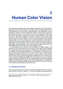
Figure 1: We take an high-dynamic-range image and predict perceptual lightness, colorfulness, and hue attributes. Based on these attributes, we can reproduce the perceptual appearance of the original image on different media, such as a low-dynamic-range display.

Abstract

recent color appearance models [CIE 1998; Moroney et al. 2002] are mainly derived from this data set and, as a result, are geared towards low luminance levels. However, with the recent advent of high-dynamic-range (HDR) images and very bright displays [Seetzen et al. 2004], a generalized color appearance model is much needed. But without the appropriate psychophysical data, no such model can be derived. Our goal is to derive such a generalized model of human color vision, which predicts perceptual color appearance under extended luminance levels (from low photopic levels to very high levels). We have therefore conducted a new set of psychophysical experiments in order to measure perceptual attributes of the color appearance for much higher levels of luminance (up to about 16,860 cd/m2 , corresponding to white paper in noon sunlight) using a specially designed high-luminance display. This allows us to derive a new generalized color appearance model that models the photopic visual response range and which adapts to different dynamic levels. In contrast to previous CAMs, our model is simple and yet achieves a significantly higher prediction accuracy. Our main contributions are: the psychophysical measurement of color perception under extended luminance levels, and a generalized color appearance model for extended luminance levels.

Display technology is advancing quickly with peak luminance increasing significantly, enabling high-dynamic-range displays. However, perceptual color appearance under extended luminance levels has not been studied, mainly due to the unavailability of psychophysical data. Therefore, we conduct a psychophysical study in order to acquire appearance data for many different luminance levels (up to 16,860 cd/m2 ) covering most of the dynamic range of the human visual system. These experimental data allow us to quantify human color perception under extended luminance levels, yielding a generalized color appearance model. Our proposed appearance model is efficient, accurate and invertible. It can be used to adapt the tone and color of images to different dynamic ranges for crossmedia reproduction while maintaining appearance that is close to human perception. Keywords: color appearance, psychophysics, color reproduction.

1

Introduction

Color is caused by the spectral characteristics of reflected or emitted radiance, which makes it seemingly easy to understand as a physical quantity. However, color is really a perceptual quantity that occurs in one’s mind, and not in the world. Therefore, the physical spectrum is commonly decomposed into perceptual quantities using physiological and psychophysical measurements that try to quantify the human visual system; e.g., the CIE 1931 standard colorimetric observation [CIE 1986]. Such color spaces commonly try to ensure that equal scale intervals between stimuli represent approximately equally perceived differences in the attributes considered. Color appearance models (CAMs) additionally try to model how the human visual system perceives colors under different lighting conditions, e.g., against different backgrounds. Many of the psychophysical measurements necessary for CAMs have been conducted in recent decades. Unfortunately, available data are geared towards the perceptual appearance of reflective photographic images and backlit advertisements, which generally have low luminance levels. For instance, the LUTCHI appearance experiments [Luo et al. 1993] were carried out with luminances mainly under about 690 cd/m2 — except for only four color samples between 1000 and 1280 cd/m2 . Perceptual color attributes of

2

Background on Color Appearance

Müller’s zone theory of trichromatic vision [Müller 1930] is commonly used as a basis for deriving computational models of human vision. It describes how the combined effect of retina, neurons, nerve fibers, and the visual cortex constitutes color perception (Fig. 2). We will briefly outline the theory here, before moving on to color appearance models.

2.1

Zone Theory

The retina features cones and rods with different spectral sensitivity. Long (L), middle (M), and short (S) cones are stimulated by approximately red, green, and blue wavelengths respectively, while the rods have achromatic sensitivity. The ratio of the numbers of the three cone types varies significantly among humans [Carroll et al. 2002], but on average it can be estimated as 40:20:1 (L:M:S). 2.1.1

Cone Adaptation

In the first stage of the visual system, the eye adapts to the observed brightness level. Two adaptation mechanisms control the effective cone response. The pupil changes size and controls the amount of light reaching the retina to a limited extent. In addition to physical adaptation, the retina itself adapts physiologically. Based on measurements of cone responses of primates under vary-

1

To appear in the ACM SIGGRAPH conference proceedings

Visible Spectrum

Fovea

Color Perception

L cone

• Absolute Quantity: 1. Brightness (Strength of A) 2. Hue (Ratio of C1 to C2-C3) 3. Colorfulness (Strength of C1 and C2-C3) • Relative Quantity: Lightness/Chroma/Saturation

M cone S cone Rod (a)

Retina

(b)

A

Brightness

C1 (R-G)

(+) R, (-) G

C2-C3 (Y-B)

(+) Y, (-) B

Neurons

Nerve Fiber

(c)

C2 = M − S and C3 = S − L, that is, C2 − C3 . The ratio of C1 and C2 − C3 causes a hue sensation in our visual cortex, and their strength conveys colorfulness. Brightness, hue, and colorfulness are the fundamental attributes of color sensation. They can be used to derive relative quantities that model human color perception. The ratio of a surface’s brightness A and the brightness An of the reference white defines the lightness sensation [Land and McCann 1971]. Setting a surface’s colorfulness in proportion to the reference brightness An yields chroma. Similarly, comparing a surface’s colorfulness to its own brightness level provides the saturation sensation.

Visual Cortex

Figure 2: Schematic illustration of human color vision based on the zone model [Müller 1930]. Light enters through the pupil and stimulates cones and rods. The given stimulus is sensed by longand middle-wave cones in the fovea, and short-wave cones and rods outside the fovea (a). The strengths of the four responses are combined to yield achromatic brightness, and the ratio and strength of the C1 (L − M) channel and the combined C2 (M − S) and C3 (S − L) channels yield the hue and colorfulness sensations. The signals travel along the nerve fiber, are merged into one image, and causes the final visual sensation at the visual cortex (c).

2.2

A color appearance model (CAM) is a numerical model of the human color vision mechanism. Common CAMs largely follow the zone theory by modeling human color vision as a four-stage procedure, shown in Fig. 4, comprising chromatic adaptation, dynamic cone adaptation, achromatic/opponent color decomposition, and computation of perceptual attribute correlates. Generally, CAMs take tristimulus XY Z values (of the color to be perceived) and parameters of the viewing condition to yield perceptual attributes predicting the perceived color (commonly lightness, chroma, and hue). CAMs mostly differ in the specific functions that transform color quantities across these four stages, the quality of their prediction, and the different viewing conditions that can be modeled. Popular models are the simple CIELAB model, RLAB [Fairchild 2005], Hunt94 [Hunt 1994], CIECAM97s [CIE 1998], up to the recent and currently widely accepted CIECAM02 [Moroney et al. 2002].

ing (flashed) incident retinal light levels I of up to 106 td (Troland units: luminance in cd/m2 × pupil area in mm2 ), Valenton and Norren [1983] found that the response satisfies the Michaelis-Menten equation [Michaelis and Menten 1913] (Eq. 1), effectively compressing the response. Normalizing the cone response V by the maximum physiological cone response Vm , they derive a general response function: V In , (1) = n Vm I + σn where n was found to be 0.74 and σ was found to depend directly on the adaptation luminance (varying from 3.5 to 6.3 log td), which shifts the response curve along the intensity axis, see Fig. 3. In contrast, Boynton and Whitten [1970] assume σ to be constant and that all sensitivity loss is caused by response compression and pigment bleaching, which is the basis of many CAMs, such as Hunt94, CIECAM97s, and CIECAM02 [Hunt 1994; CIE 1998; Moroney et al. 2002]; however, we will demonstrate that for accurate prediction of lightness, σ should be allowed to vary. Humans perceive object colors as constant under different illumination; this effect is called color constancy. It is believed that the underlying mechanism is caused by a slightly different adaptation of each cone type but the details are still debated. It may even be a combination of cone adaptation and processing in the cortex. 2.1.2

3

Total response, V (µV)

According to the zone theory, the cones’ and rods’ responses are transformed into three neural signals, which are passed along the nerve fibers. A weighted combination of the three cone- and rodresponse yields one achromatic signal A that is perceived as brightness. Color information is transformed in the form of two difference signals: the red/green opponent color attribute is the difference of the L and M cone sensations, C1 = L − M; the yellow/blue opponent color attribute is the difference of the two difference signals 800 600 DA 2 3

4

5

6

200 0

-200 1

2

3 4 5 Log intensity, I (log td)

6

Related Work

Color Appearance Models Many different color appearance models have been proposed over the years. We will briefly review common ones. CIECAM02 [Moroney et al. 2002] is considered one of the most complete and accurate color appearance models. It follows the zone theory closely. First, chromatic adaptation is performed using CIECAT02, which supports varying degrees of adaptation. The resulting white-adapted XY Z values are then normalized. The cone response is modeled using Eq. 1, but with a fixed σ , which causes the response to be similar to a power function. The opponent color decomposition follows Section 2.1.2 closely. The final attributes include lightness, brightness, chroma, colorfulness, hue and saturation. CIECAM02 can model different surroundings and adaptation levels. Generally, its performance is good. However, as we will see, it has difficulties with higher luminance levels, both in terms of colorfulness as well as lightness. We partially attribute this to the fact that input XY Z values are normalized, which seems to lose important information. CIECAM97s [CIE 1998] is similar in spirit to CIECAM02 but is much more complex. Its practical applicability is limited since, for instance, the color appearance transform is non-invertible and the prediction of saturation is problematic. CIECAM02 is in many respects its simpler but more powerful successor. CIELAB is a very simple color appearance model that is purely based on XY Z tristimulus values. Chromatic adaptation is performed by dividing XY Z values by normalized white point values XY Zw , and the cone response is modeled as a cube root in Y . Only lightness, chroma, and hue are predicted. It does not model any adaptation to different backgrounds or surround changes. Despite these simplifications, it still performs well. RLAB [Fairchild 2005] is an improved version of CIELAB in that it models different viewing conditions. In particular, it supports different media and different surround conditions. Chromatic adaptation is performed in LMS cone color space, but color attributes are still computed from white-adapted XY Z values.

Trichromatic Vision

400

Color Appearance Models

7

Figure 3: Cone response (V ) vs. intensity (log I) curves in the presence of adapting background illumination from dark adapted luminance (DA) to brighter adaptation luminances (2, 3, 4, 5, and 6 log td). Adapted from [Valeton and van Norren 1983].

2

To appear in the ACM SIGGRAPH conference proceedings

X Chromatic Adaptation Transform

Y Z

Xc

L

L’

Yc

M

M’

Zc

S

S’

Achromatic (A)

Lightness (J)

L:M:S

Colorfulness (M)

Opponent (a, b)

XYZW

Chroma (C)

Saturation (s)

Hue Quadrature (H)

Hue (h)

La

Outputs

Inputs

Chromatic Adaptation

Brightness (Q)

Cone Responses

Color Decomposition

Color Appearance

Figure 4: Color appearance models roughly follow these four stages. First, the incoming spectrum, sampled as an XY Z triple, is transformed for chromatic adaptation. This is usually done in a specialized color space (though not always). Then, the white-adapted XY Zc is transformed into the cone color space, where a cone-response function is applied (commonly a power or hyperbolic function). After that, the signal is decomposed in the achromatic channel A and the color opponent channels a and b. The perceptual correlates are based on these three channels. This is where color appearance models differ most, as a large range of functions are applied to yield perceptual values.

4

Perceptual Experiments Most color appearance models are based on the LUTCHI experimental data [Luo et al. 1991]. The goal was to quantify color appearance on different media and under different viewing conditions to form a rigorous basis for the development of color appearance models. For each medium (eight different ones, from CRT to transparencies) and viewing condition (different background levels, peak luminance, etc.), observers were presented with many color patches. For each patch, the observers estimated the patch’s lightness (relative to reference white), its hue, and its colorfulness. In addition, actual physical measurements of each patch were collected. This experimental data enables the derivation of a mapping from physical measurements to perceptual estimates, which constitutes a color appearance model. While the LUTCHI experiment comprises a large variety of media and viewing conditions, it was geared towards low luminance levels with most experiments carried out under 690 cd/m2 .

Psychophysical Experiments

In order to quantify actual perceptual color appearance, we have conducted a magnitude estimation experiment. Observers are successively presented with a large number of colored patches, for which they have to estimate lightness, hue, and colorfulness values. Across different phases of the experiment, parameters influencing the estimates are changed: background level, luminance (and color temperature) of the reference white, as well as ambient luminance. We designed our psychophysical experiment in a similar way to the LUTCHI experiment, which allows us to leverage their existing data. However, our experiment differs from LUTCHI by including high luminance levels of up to 16,860 cd/m2 .

4.1

High-Luminance Display

In order to span an extended range of luminance levels, we built a custom display device which is capable of delivering up to approximately 30,000 cd/m2 , see Fig. 5. The setup consists of a light

Tone Mapping Tone mapping is related to color appearance modeling as it tries to preserve the perception of an image after remapping to a low-luminance display; however, generally only tone (and not colorfulness) is considered. Early work applied a global curve to a high-dynamic-range image [Ward 1994; Tumblin and Rushmeier 1993], whereas later work allows for spatial variation [Reinhard et al. 2002; Durand and Dorsey 2002]. Commonly, tonemapping algorithms only modify lightness while keeping the color channels untouched (e.g., in CIEYxy only Y is modified), which may lead to perceptually flawed color reproduction (washed out colors), as has been recently shown [Mantiuk et al. 2009]. Mantiuk et al. [2009] demonstrate how to improve color reproduction in tone mapping, based on psychophysical experiments. Akyüz and Reinhard [2006] propose to combine parts of the CIECAM02 color appearance model with tone mapping, in order to yield a better color reproduction. However, tone compression was still performed only on luminance (Y in the Y xy domain). In contrast, our CAM can be used to keep the perceived colorfulness and hue of color samples as close to the original as possible during tone-mapping.

Filter Slot

Fireglass

LCD Unit

Filter Unit UV Filter ND Filters Color Correct Filter Diffuser + LCD / Trnsp.

HMI Bulbs (2 x 400W)

Figure 5: Left: The high-luminance display with LCD unit (exchangeable for transparencies on a diffuser) and empty filter slot. Top Right: Schematic of the filter unit. Bottom Right: LCD and transparency viewing pattern observed by a participant. box, powered by two 400 W HMI bulbs, transmitting light through a filter ensemble followed by either a 19LCD panel (original backlight removed), or a diffuser onto which transparencies are placed. The light source spectrum conveniently resembles fluorescent backlights, with a color temperature of 6500 K. Moreover, HMI bulbs stay cool enough to keep the LCD panel from overheating. Light Source Color Temperature We can modify the color temperature of our light source by placing Rosco temperature-changing filters inside the light box. Our experiments use 2000 K, 6500 K, and 8000 K with the LCD, and 6000 K with transparencies. Luminance Level Peak luminance (and with it the luminance of the reference white, as well as of all color samples) is controlled by placing additional neutral density (ND) filters into the light box (which preserves amplitude resolution). Combination of different ND filters creates the peak luminances of approximately 50, 125, 500, 1000, 2200, 8500, and 16860 cd/m2 used in our experiment.

Image Appearance Advanced models exist that try to combine CAM with spatial vision. Ferwerda et al. [1996] proposed a computational model of human vision that includes spatial adaptation. It was mainly based on previous threshold experiments; accurate color perception was not modeled. Pattanaik et al. [1998] improved on these results using a multiscale model of adaptation and spatial vision, combined with a simplified version of CIECAM97s. Johnson and Kuang et al. [2003; 2007] introduced an image appearance model, which is essentially a combination of CIECAM02 with tone mapping [Durand and Dorsey 2002]. It produces reasonable results, however CIECAM02 has difficulty at predicting high-level luminances, as mentioned before. Our aim is not to derive a full image appearance model; instead, we want to derive a pure CAM that enables accurate prediction of color perception.

3

To appear in the ACM SIGGRAPH conference proceedings Phase 1 2 3 4 5 6 7 8 9 10 11 12 13 14 15 16 17 18 19

Display Options When used with the LCD, the maximum displayable luminance is 2,250 cd/m2 (similar to the Dolby HDR display [Dolby 2008]), with a contrast ratio of about 1:1000. Owing to the 8-bit LCD, the amplitude resolution is only 256 steps (less than for a real HDR display [Seetzen et al. 2006]). However, this is not critical, as the experiment only requires sparse sampling of the color space. For transparencies, the maximum luminance reaches 30,000 cd/m2 , with virtually arbitrary contrast and amplitude resolution. Calibration Using a Specbos Jeti 1200 spectroradiometer, we color-calibrated the LCD version of our display. We further measured the spectra of all displayed color patches (LCD and transparencies), as well as background and reference white. The reference white was re-measured at the beginning and at the end of each day to ensure repeatability. Over the two-week period of our experiments, we recorded only an insignificant variation of about 3% in luminance and a 1% decrease in color temperature.

4.2

4.3

The basic setup for our perceptual measurements is adapted from the LT phases (cut-sheet transparencies) of LUTCHI [1993]. A participant is asked to look at a color patch, presented next to a reference white patch and a reference colorfulness patch (with a colorfulness of 40 and lightness of 40), as shown in the center of Fig. 6a. The viewing pattern is observed at 60 cm distance, normal v' 0.4

0.2

(b)

Spectral Locus LCD Color Patches Trans. Color Patches 0

0.2

0.4

0.6

Peak Lumin. 44 cd/m2 123 cd/m2 494 cd/m2 521 cd/m2 563 cd/m2 1,067 cd/m2 1,051 cd/m2 2,176 cd/m2 2,189 cd/m2 2,196 cd/m2 2,205 cd/m2 2,241 cd/m2 1,274 cd/m2 1,233 cd/m2 2,201 cd/m2 8,519 cd/m2 8,458 cd/m2 16,860 cd/m2 16,400 cd/m2

Backgrnd. 24% 21% 0% 24% 87% 0% 22% 0% 12% 23% 55% 95% 21% 19% 23% 6% 21% 5% 22%

Ambient dark dark dark dark dark dark dark dark dark dark dark dark dark dark average dark dark dark dark

Experimental Procedure

A crucial point of psychophysical measurements through magnitude estimation is that each observer clearly understands the perceptual attributes being judged. Each observer completed a 3-hour training session with the actual viewing pattern (using a different set of color patches) to develop a consistent scale for each of the required perceptual attributes (lightness, colorfulness, and hue). For data compatibility, the same scaling unit and instructions were used as for the LUTCHI dataset [Luo et al. 1993]. We employed six fully trained expert observers, all of whom were research staff from our institution, who had passed the Ishihara and City University vision tests for normal color vision. Each observer spent around 10 hours on the experiment, usually distributed over two days. At the beginning of each phase, observers spent about 5–30 minutes adapting to the viewing conditions. Then, each color sample was shown in a random order and the participants had to estimate three perceptual attributes: lightness, for which observers used a fixed scale from 0 (imaginary black) to 100 (reference white); hue, where observers were asked to produce a number indicating the hue using neighboring combinations among four primaries — redyellow (0–100), 100–200 (yellow-green), 200–300 (green-blue), 300–400 (blue-red); and colorfulness, where observers used their own open scale, with 0 being neutral and 40 equaling the anchor colorfulness. The participants entered the data using a keyboard. After each phase, participants were asked to judge the colorfulness of the reference colorfulness patch of the next phase relative to the previous one in order to allow inter-phase data analysis.

0.6

(a)

Type LCD LCD LCD LCD LCD LCD LCD LCD LCD LCD LCD LCD LCD LCD LCD Trans. Trans. Trans. Trans.

Table 1: Summary of the 19 phases of our experiment. In each phase, 40 color samples are shown. Each participant made a total of 2,280 estimations, which took around 10 hours per participant.

Stimuli

0

Light 5935K 6265K 6265K 6265K 6197K 6197K 6197K 6390K 6392K 6391K 6387K 6388K 7941K 1803K 6391K 5823K 5823K 5921K 5937K

u'

Figure 6: (a) Viewing pattern observed by participants. (b) Color coordinates of the 40 LCD and transparency patches (CIE uv). to the line of sight, such that each of the roughly 2× 2 cm2 patches covers about 2, and the whole display about 50 of the field of view. The background is black or gray, with 32 random decorating colors at the boundary, mimicking a real viewing environment. We selected a total of 40 color patches as stimuli, carefully chosen to provide a good sampling of the available color gamut and to provide a roughly uniform luminance sampling. Figure 6b shows the distribution of these 40 patch colors for each device. The sets for the LCD and transparency setup are different, as it is neither easy to match their spectra nor necessary for the experiment.

4.3.1

Discussion

The reference colorfulness patches were chosen to have a colorfulness of 40 according to the CIELAB color space. It should be noted that the reference colorfulness is only meant to anchor the estimates, and as such any color or any value can be chosen. As mentioned above, participants were asked to rate inter-phase colorfulness changes with a memory experiment. The results are implicitly shown in Fig. 7, where (a) and (b) plot the average colorfulness for different phases. The change in colorfulness between phases stems from this experiment. It should be mentioned that there are some distinct differences to previous experiments. The LUTCHI data set was geared towards reflective surfaces and low-luminance conditions — no data are available for extended luminance levels. As a result, CAMs derived only from LUTCHI cannot robustly model color appearance under higher luminance levels. For instance, this can be seen in Fig. 14.

Since the perception of lightness, colorfulness, and hue is strongly correlated with parameters such as luminance range, reference white, background level, and surround condition [Stevens and Stevens 1963; CIE 1981; Luo et al. 1991; Luo and Hunt 1998; Hunt et al. 2003], our study explores relevant slices of this high-dimensional space. We partition the experiment into different phases, with a specific set of parameters in each phase (see Table 1). We primarily focus on the influence of luminance range and background level on color perception as these two dimensions are known to have the strongest perceptual influence [Luo et al. 1991]. We performed experiments up to a peak luminance of 16,860 cd/m2 ; higher luminance levels were abandoned as too uncomfortable for the participants. As previous color experiments have already covered low luminance, we conducted only a few low-luminance experiments (phases 1–5 in Table 1) to verify consistency.

4

To appear in the ACM SIGGRAPH conference proceedings 4.4

Data Analysis

indicated by the observers in post-experiment interviews. This was not found in the first LUTCHI experiment (low luminance levels) [Luo et al. 1991], but a similar effect was reported later on [Luo et al. 1993]. Hue is very constant with regard to variation in luminance, background, and surround, which is consistent with previous data. Most of our findings are consistent with the LUTCHI dataset, and similar trends can be observed in both datasets. Additionally, the LUTCHI dataset indicates that lightness perception is mediadependent: darker colors appear lighter on luminous displays (e.g., LCD) than on reflective media (e.g., paper) [Luo et al. 1993]. Three observers repeated two phases of the original experiment in order to judge repeatability. The average CV between the two experiments was 11.83% for lightness, 22.82% for colorfulness, and 11.42% for hue. This is consistent with previous experiments and with participants’ comments that colorfulness is difficult to judge.

For lightness and hue estimates, all observers had to use the same numerical scale with fixed end points. This forced the observers to use a partition technique rather than pure magnitude estimation [Stevens 1971]. Consequently, we can compute the arithmetic mean between all observers. Note that for hue, the scale is circular and care needs to be taken when averaging. For colorfulness scaling, the observers applied their own arbitrary scale (pure magnitude estimation [Bartleson 1979; Pointer 1980]). According to Stevens [1971], the appropriate central tendency measure for magnitude estimation is the geometric mean, but only after relating the observers’ responses to each other (since observers use their individual scales). We follow the same procedure as Luo et al. [1991] and map each observer’s responses to the mean observer. The coefficient of variation (CV), i.e., the RMS error with respect to the mean, was mainly used as a statistical measure to investigate the agreement between any two sets of data.

4.5

5

Findings

70

80

60

70

Perceived Scales

Perceived Scales

Before describing our model, we will summarize important findings and trends observed in our data. The average perceived lightness increases with increased peak luminance (fixed background ratio), see Fig. 7a. We note that the perceived lightness of the mediumlight colors (not dark, not bright) mainly increases, which can be seen in Fig. 7c (plot of lightness with respect to CIELAB L* values). This means that the shape of the perceived lightness curve changes. In contrast, when the background luminance level increases (Fig. 7b), the average perceived lightness decreases (mainly dark and medium-light colors), as shown by Bartleson and Breneman [1967]. Colorfulness shows a similar trend. At higher luminance levels perceived colorfulness increases (Fig. 7a and d), which is known as the Hunt effect [Hunt 2004]. Further, colorfulness decreases when background luminance increases (Fig. 7b), which was also

30

20

Perceived Lightness Perceived Colorfulness

10

10

100

1,000

Perceived Lightness Perceived Colorfulness

20 10

10,000

Luminance (fixed Back.) [cd/sqm]

100

0 0%

(b)

20%

40%

60%

80%

100%

Background Level (fixed Lumin.)

5.2

Perceived Colorfulness

140

Perceived Lightness

100

60

40

20

43 cd/sqm 2,196 cd/sqm

80 60 40

43 cd/sqm 2,196 cd/sqm

20

0

0

0

20

40

60

CIELAB L*

80

100

(d)

0

20

40

60

80

100

CIELAB C*

120

Cone Response

The physiological experiments by Valenton and Norren [1983] demonstrate that the cone response of primates follows a sigmoidal curve, which is influenced by the level of adaptation of the eye. There are good reasons to believe that the cones of human eyes respond in a very similar manner. Tristimulus values are first transformed into LMS cone space using the Hunt-Pointer-Estévez (HPE) transform [Estévez 1979]. We then model the cones’ absolute responses according to Eq. 1:

120

80

Chromatic Adaptation

Humans perceive object colors as constant under different illumination (color constancy). This is commonly simulated using models of chromatic adaptation [Li et al. 2002]. As the focus of our experiments was not on chromatic adaptation, we simply adopt the CIECAT02 chromatic adaptation transform [Moroney et al. 2002] that has been shown to work well. It takes the incident (absolute) XY Z D50 values and transforms them to new XY ZC values, accounting for chromatic adaptation based on the reference white. It is important to note that, in contrast to previous models, we do not normalize the signal but keep its absolute scale; i.e., the whiteadapted XY ZC has the same luminance as the original XY Z.

40

30

0

(c)

5.1

50

40

(a)

We propose a new color appearance model that closely follows the zone theory in order to perform well under high-luminance conditions. The model consists of three main components: chromatic adaptation, cone responses, and cortex responses for each perceptual color attributes. It aims to accurately predict lightness, colorfulness and hue, including the Hunt effect (colorfulness increases with luminance levels), the Stevens effect (lightness contrast changes with different luminance levels), and simultaneous contrast (lightness and colorfulness changes with background luminance levels). Additional correlates of brightness, chroma, and saturation will be derived as well.

60

50

High-Luminance Color Appearance Model

140

L0 =

Figure 7: (a) Lightness and colorfulness perception for different luminance levels (phases 1, 2, 4, 7, and 10). (b) Lightness and colorfulness perception for different background levels (phases 9–12). (c) Qualitative comparison of lightness at two different luminance levels. (d) Qualitative comparison of colorfulness at two different luminance levels. We plot the perceived values of the 40 patches in (c) and (d) against CIELAB L* and C* of the physical measurements, as it shows their variation clearly; other choices (such as plotting against physical luminance) lead to the same conclusions.

Lnc M nc Snc 0 0 , M = , S = . n n Lnc + Lac M nc + Lac Snc + Lanc

(2)

We have only replaced the σ from the original equation (where it was given in Troland units) with the absolute level of adaptation La measured in cd/m2 (both units are related almost linearly for the working range of the adaptation level). The adaptation level should ideally be the average luminance of the 10◦ viewing field (it serves as an input parameter to our model). The parameter nc is known only for primates, hence we have derived it from our experimental data as nc = 0.57.

5

To appear in the ACM SIGGRAPH conference proceedings 5.3

Achromatic Attributes

data. We further know that colorfulness should increase with luminance level (Hunt effect). We found the relationship between chroma (as defined above) and colorfulness to be linear in the logarithm of the reference white luminance Lw :

The cone response then is converted into an achromatic signal A by averaging the contribution of each type of cone. The actual weighting between the three cone responses is not known exactly, but is generally believed to be 40:20:1 [Vos and Walraven 1971]. The signal A is then defined as: A = (40L0 + 20M 0 + S0 )/61.

M = C · (αm log10 Lw + βm ).

(3)

Lightness is (very roughly) defined as the ratio between the achromatic signal and the achromatic signal of reference white Aw , since the observer was asked to relate the two. Plotting the ratio A/Aw against perceived lightness values, yields a consistent inverse sigmoidal shape. The goal is to yield a 1:1 mapping between predicted and perceived lightness, which we achieve by applying an inverse hyperbolic function to yield lightness J 0 : A
J0 = g , (4) Aw " #1/n j with n −(x − β j )σ j j g(x) = . (5) x − βj − αj

π

This hue angle (0◦ –360◦ ) could be used directly as a prediction of perceived hue, however, perceptual hue quadrature [Moroney et al. 2002] (H = huequad(h)) has been shown to improve accuracy, which we adopt in our model as well. We kindly refer the reader to [Moroney et al. 2002] for the exact formula.

The values of the parameters are derived from our experimental data, yielding α j = 0.89, β j = 0.24, σ j = 0.65, and n j = 3.65. It is interesting to note that J 0 may yield values below zero, in which case it should be clamped. This corresponds to the case where the observer cannot distinguish dark colors from even darker colors anymore. As already mentioned before, the perceived lightness values vary significantly with different media, even though the physical stimuli are otherwise identical. As with others [Fairchild 2005; Hunt 1994], we have decided to incorporate these differences explicitly in our model in order to improve lightness prediction, yielding a mediadependent lightness value: J = 100 · [E· (J 0 − 1) + 1] ,

5.5

Inverse Model

For practical applications, it is necessary to be able to invert a color appearance model; i.e., one needs to derive physical quantities (absolute XY Z), given perceptual lightness, colorfulness, hue and viewing parameters as input. For instance, tone-mapping of HDR images is achieved by first taking an absolute HDR radiance map (containing physically meaningful XY Z values) and applying the CAM, which yields perceptual attributes (JMh). These attributes are then mapped to absolute XY Z for a specific target display and target viewing condition by applying the inverse model. Finally, XY Z coordinates are transformed into device-dependent coordinates (e.g., sRGB) for display. Our model is analytically invertible, see the appendix for details, and can thus be used for tone-mapping and other practical applications such as cross-media reproduction.

(6)

where the parameter E is different for each medium. A value of E = 1.0 corresponds to a high-luminance LCD display, transparent advertising media yield E = 1.2175, CRT displays are E = 1.4572, and reflective paper is E = 1.7526. These parameters were derived from the LUTCHI data set as well as ours. Brightness was not measured in our experiments. However, the LUTCHI data set contains a few phases with both lightness and brightness measurements, which indicate that these two properties have a linear relationship in the log-log domain. We therefore define brightness as: Q = J · (Lw )nq . (7)

6

Results

The following provides a quantitative analysis of our model. We have applied our model, as well as CIELAB, RLAB, and CIECAM02 to our perceptual data. The main result can be found in Fig. 8. Our prediction in terms of lightness is very consistent and the CV value is about as large as the repeatability CV value for a human observer, which indicates that it will be difficult to achieve better lightness prediction than what our model achieves. Other models achieve a less accurate prediction and, importantly, their prediction quality fluctuates considerably between phases. Colorfulness is also predicted very consistently by our model and is generally much better than the other models. As before, the CV value is similar to the CV value between two repeated runs of the same experiment. The other models’ performance varies significantly, not only between models, but also between phases. Hue is predicted very similarly between all models, even the simple CIELAB performs well. It is interesting to look at a particular phase in more detail. Figure 9 shows plots that detail lightness, colorfulness and hue as estimated by our model versus the actual perceived values from our experiment. Our lightness, colorfulness, and hue prediction are very much along the diagonal, indicating that our model covers the dominant perceptual phenomena. However, CIECAM02 incorrectly estimates lightness yielding values that form a curve off the diagonal. This effect can be noticed in other phases as well: the predicted lightness forms a curve instead of a diagonal line as would be expected.

The parameter is driven from experimental data and yields nq = 0.1308.

5.4

(11)

From this we can derive parameters for colorfulness as well as chroma based on our data and the constraint that chroma does not change with luminance: αk = 456.5, nk = 0.62, αm = 0.11, and βm = 0.61. The other remaining quantity is saturation, which by definition is the colorfulness relative to its own brightness: r M s = 100 · (12) Q The hue angle is computed by taking the arctan of a and b: 180 tan−1 (b/a) (13) h=

Chromatic Attributes

The eye is believed to compute opponent signals a and b, which are based on differences between the cone responses. We adopt previous psychophysical results on how the responses are combined together [Vos and Walraven 1971], yielding: 1 (11 · L0 − 12 · M 0 + S0 ) Redness − Greenness (8) a = 11 1 0 (L + M 0 − 2 · S0 ) Yellowness − Blueness (9) b = 9 Chroma C is the colorfulness judged in proportion to the brightness of reference white, i.e., it should be independent of luminance Lw . It is commonly based on the magnitude of a and b: p  nk C = αk · a2 + b2 . (10) Note that it is only possible to optimize the parameters αk and nk after modeling colorfulness, for which we have actual perceptual

6

To appear in the ACM SIGGRAPH conference proceedings 40 30 25 20 15 10 5

CVs of Colorfulness

0

1

2

3

4

5

6

7

8

9

10

11

12

13

14

15

16

17

19

Phases

50 45 40 35 30 25 20 15 10 5 0

Colorfulness Hue

35 30 25 20 15 10 5 0 CIELAB

1

2

3

4

5

6

7

8

9

10

11

12

13

14

15

16

17

18

RLAB

CIECAM02

Our Model

Figure 10: This figure compares the average CV error (and standard deviation) of estimated lightness, colorfulness, and hue when applied to several phases of the LUTCHI dataset. In particular, we use the transparency phases, reflective media phases, and CRT phases. Our model achieves the best overall prediction. Further, the variation in error is rather small for our lightness and colorfulness prediction, indicating that our model performs consistently.

CIELAB RLAB CIECAM02 Our Model

19

Phases

35

CIELAB RLAB CIECAM02 Our Model

30 CVs of Hue

18

Lightness

40

Aver. CVs of Estimation

CVs of Lightness

45

CIELAB RLAB CIECAM02 Our Model

35

25 20 15 10 5 0

1

2

3

4

5

6

7

8

9

10

11

12

13

14

15

16

17

18

19

Phases

Figure 8: We compare all 19 phases of our experiment in terms of lightness, colorfulness, and hue prediction error (CV error) with CIELAB, RLAB, and CIECAM02. Our model performs consistently better than the other models in terms of lightness. Colorfulness prediction is better in almost all cases. Hue prediction is very similar to the other models, even though CIECAM02 is minimally better at lower luminances.

Figure 11: Our model can be used to match the color appearance on different media. Starting from a radiometrically calibrated XY Z float image [Kim and Kautz 2008], the left image printed on paper will appear very similar to the right image when displayed on an LCD (assuming calibrated devices in dim viewing conditions).

We further investigate how our model predicts the data from the LUTCHI data set. Figure 10 summarizes the result. We ran all four models on a large number of phases from that dataset (transparency, reflective media (paper), and CRT). Our model outperforms the other CAMs in terms of lightness, colorfulness, and hue, even though the LUTCHI dataset was not the main basis for the derivation of our model. Once more, our lightness and colorfulness prediction is very consistent (small standard deviation in CV). Prediction quality of hue varies as much as CIECAM02’s prediction, which is not surprising as we use the same hue computation. In Figure 11, we demonstrate media-dependent reproduction. The left image printed on paper is perceptually equivalent to the right image displayed on an LCD display (assuming a calibrated device in dim viewing conditions). If both are viewed on an LCD display, the left image appears brighter. This is due to the fact that luminance and colorfulness perception for paper decreases, and our CAM compensates for it. 100

140

Perceived Colorfulness

Perceived Lightness

16,400 cd/sqm

400

16,400 cd/sqm

120

80

300

CIECAM02

20

Our Model

Perceived Hue

40

250

80

200

60

150

40

100

CIECAM02

20

0

20

40

60

80

Estimated Lightness

100

CIECAM02

50

Our Model

0

0

Figure 12 demonstrates that our CAM can be used to match appearance of images with different backgrounds. The two images appear identical even though the one on the right is actually lighter and more colorful. This is achieved by modifying the target adaptation level (white background ≈ higher adaptation luminance) when applying our CAM. Figure 13 compares the use of our color appearance model for tone-mapping with Reinhard et al.’s method [2002] and iCAM06 [Kuang et al. 2007]. Our model’s results are consistent throughout with good luminance compression. Colors are slightly more saturated than with the other two models, which is due to our model preserving the original colorfulness impression but at lower target luminance levels. Figure 14 compares tone-mapping with CIECAM02, iCAM06 and our model. As can be seen, CIECAM02 is not designed to handle HDR images. We have conducted a pilot study, as shown in [Kuang et al. 2007], letting participants compare the real-world scene from Fig. 14

16,400 cd/sqm

350

100

60

Figure 12: The two color charts will appear similar (assuming calibrated display with a gamma of 2.2 in dim viewing conditions). When comparing the two images without the backgrounds, it can be seen that the right color chart is actually lighter and more colorful.

Our Model

0 0

20

40

60

80

100

120

Estimated Colorfulness

140

0

50

100 150 200 250 300 350 400

Estimated Hue

Figure 9: Comparison of the prediction of all 40 samples (estimated lightness using our model) for one particular phase (16,400 cd/m2 ) against perceived lightness from the user study. It can be seen that our model achieves very good lightness, colorfulness and hue prediction. CIECAM02 is not able to predict lightness with the same accuracy.

7

To appear in the ACM SIGGRAPH conference proceedings 2

3

* Images courtesy of [1] Paul Debevec, [2] Yuanzhen Li, [3] Martin Cadik, [4] Dani Lischinski, [5] Greg Ward, and [6] Industrial Light & Magic. 4 5 6

(c) Our Model

(b) iCAM06

(a) Reinhard et al.

1

Figure 13: Absolute HDR radiance maps are tone-mapped using Reinhard et al.’s tone-mapping algorithm [2002], the iCAM06 image appearance model [Kuang et al. 2007], and our color appearance model. The target display is assumed to be sRGB with a peak luminance level of 250 cd/m2 and a gamma of 2.2 (dim viewing conditions, adapting luminance is assumed to be 10% of peak luminance). For Reinhard et al.’s and our method, we simulate chromatic adaptation as outlined in Section 5.1; iCAM06 uses its own spatially-varying model. of color appearance and as such do not try to describe how human vision actually works.

8

We have presented a new color appearance model that has been designed from the ground up to work for an extended luminance range. As no color perception data was available for high luminance ranges, we have first conducted a large psychophysical magnitude experiment to fill this gap. Based on our data, as well as previous data, we have developed a model that predicts lightness, colorfulness and hue at a high accuracy for different luminance ranges, levels of adaptation, and media. In contrast to other CAMs, our method works with absolute luminance scales, which we believe is an important difference and key to achieving good results. We have demonstrated its usefulness for perceptually-based luminance compression of images and for cross-media color reproduction.

Figure 14: Comparison of perceptual predictions of CIECAM02 (left), iCAM06 (center), and our model (right). and its reproduction on a low-luminance display (250 cd/m2 ) using iCAM06, Reinhard et al., and our model. All 10 participants consistently ranked our reproduction as closest to reality, Reinhard et al.’s second, and iCAM06 third.

7

Conclusion

Discussion

Acknowledgements

Our psychophysical experiment and appearance model focused on the high-luminance photopic vision rather than dim (mesotopic) or dark (scotopic) vision, because our research was motivated by the advent of high-dynamic-range imaging, which deals with higher levels of luminance. Our experiment focused on the variation of luminance levels as well as background luminance. It is interesting to note here that our model does not take a separate background parameter. Our model is only driven by the adaptation luminance level (implicitly containing the background level) and the peak luminance level. In contrast, CIECAM02 uses the luminance adaptation level and the background luminance level. Our experiment did not fully investigate how the surround influences perception at high luminances. We varied the surround from dark to average for phase 15, but the influence on the perceived attributes was minimal, as observed in [Breneman 1977]. Even though our model does not have an explicit parameter for surround, its effect can be taken into account by changing the adaptation level accordingly. Furthermore, we did not fully explore chromatic adaptation, as extensive data is available from the LUTCHI experiment. We also determine the mediadependent parameter for paper, CRT, etc. from the LUTCHI data. Most of the open parameters of our model were fitted using bruteforce numerical optimization (exhaustive search for minimum). Our model does not perfectly fit the zone theory, but is inspired by it. This is not an issue, as CAMs are only computational models

We would like to thank our participants for their tremendous effort, Prof. Zhaoping Li for the use of her laboratory, and Martin Parsley and James Tompkin for proof-reading. We would like to express gratitude to the anonymous reviewers for their valuable comments.

References A KYÜZ , A. O., AND R EINHARD , E. 2006. Color appearance in high-dynamic-range imaging. J. Electronic Imaging 15, 3, 1–12. BARTLESON , C., AND B RENEMAN , E. 1967. Brightness perception in complex fields. J. Opt. Soc. Am. 57, 7, 953–957. BARTLESON , C. J. 1979. Changes in color appearance with variations in chromatic adaptation. Color Res. Appl. 4, 3, 119–138. B OYNTON , R. M., AND W HITTEN , D. N. 1970. Visual adaptation in monkey cones: recordings of late receptor potentials. Science 170, 3965, 1423–1426. B RENEMAN , E. 1977. Perceived saturation in complex stimuli viewed in light and dark surrounds. J. Opt. Soc. Am. 67, 5, 657– 662. C ARROLL , J., N EITZ , J., AND N EITZ , M. 2002. Estimates of L:M cone ratio from ERG flicker photometry and genetics. J. Vision 2, 8, 531–542.

8

To appear in the ACM SIGGRAPH conference proceedings M ORONEY, N., FAIRCHILD , M. D., H UNT, R. W. G., L I , C., L UO , M. R., AND N EWMAN , T. 2002. The CIECAM02 color appearance model. In Proc. Color Imaging Conference, IS&T, 23–27.

CIE. 1981. An analytic model for describing the influence of lighting parameters upon visual performance. CIE Pub. 19/2.1, CIE, Vienna, Austria. CIE. 1986. Colorimetry. CIE Pub. 15.2, CIE, Vienna, Austria.

M ÜLLER , G. E. 1930. Über die Farbenempfindungen. Z. Psychol., Erganzungsbände 17 and 18.

CIE. 1998. The CIE 1997 interim colour appearance model (simple version), CIECAM97s. CIE Pub. 131, CIE, Vienna, Austria.

PATTANAIK , S. N., F ERWERDA , J. A., FAIRCHILD , M. D., AND G REENBERG , D. P. 1998. A multiscale model of adaptation and spatial vision for realistic image display. In Proc. SIGGRAPH 98, 287–298.

D OLBY. 2008. Dolby’s High-Dynamic-Range Technologies: Breakthrough TV Viewing. Tech. rep., Dolby Laboratories, Inc. D URAND , F., AND D ORSEY, J. 2002. Fast bilateral filtering for the display of high-dynamic-range images. ACM Trans. Graph. (Proc. SIGGRAPH) 21, 3, 257–266.

P OINTER , M. R. 1980. The concept of colourfulness and its use for deriving grids for assessing colour appearance. Color Res. Appl. 5, 2, 99–107.

E STÉVEZ , O. 1979. On the Fundermental Data-Base of Normal and Dichromatic Colour Vision. Ph.D. thesis, University of Amsterdam.

R EINHARD , E., S TARK , M., S HIRLEY, P., AND F ERWERDA , J. 2002. Photographic tone reproduction for digital images. ACM Trans. Graph. (Proc. SIGGRAPH) 21, 3, 267–276.

FAIRCHILD , M. D. 2005. Color Appearance Models, 2nd ed. John Wiley, Chichester, England.

S EETZEN , H., H EIDRICH , W., S TUERZLINGER , W., WARD , G., W HITEHEAD , L., T RENTACOSTE , M., G HOSH , A., AND VOROZCOVS , A. 2004. High dynamic range display systems. ACM Trans. Graph. (Proc. SIGGRAPH) 23, 3, 760–768.

F ERWERDA , J. A., PATTANAIK , S. N., S HIRLEY, P., AND G REENBERG , D. P. 1996. A model of visual adaptation for realistic image synthesis. In Proc. SIGGRAPH 96, 249–258. H UNT, R. W. G., L I , C. J., AND L UO , M. R. 2003. Dynamic cone response functions for models of colour appearance. Color Res. Appl. 28, 2, 82–88.

S EETZEN , H., L I , H., Y E , L., H EIDRICH , W., W HITEHEAD , L., AND WARD , G. 2006. Observations of luminance, contrast and amplitude resolution of displays. SID Symposium 37, 1, 1229– 1233.

H UNT, R. 1994. An improved predictor of colourfulness in a model of colour vision. Color Res. Appl. 19, 1, 23–26.

S TEVENS , S., AND S TEVENS , J. 1963. Brightness function: Effects of adaptation. J. Opt. Soc. Am. 53, 3, 375–385.

H UNT, R. W. G. 2004. The Reproduction of Colour, 6th ed. John Wiley, Chichester, England.

S TEVENS , S. S. 1971. Issues in psychophysical measurement. Psychological Review 78, 426–450.

J OHNSON , G. M., AND FAIRCHILD , M. D. 2003. Rendering HDR images. In Proc. Color Imaging Conference, IS&T, 36–41.

T UMBLIN , J., AND RUSHMEIER , H. E. 1993. Tone reproduction for realistic images. IEEE Comput. Graphics. Appl. 13, 6, 42–48. VALETON , J. M., AND VAN N ORREN , D. 1983. Light adaptation of primate cones: an analysis based on extracellular data. Vision Research 23, 12, 1539–1547.

K IM , M. H., AND K AUTZ , J. 2008. Characterization for high dynamic range imaging. Computer Graphics Forum (Proc. EUROGRAPHICS) 27, 2, 691–697.

VOS , J. J., AND WALRAVEN , P. L. 1971. On the derivation of the foveal receptor primaries. Vision Research 11, 8, 799–818.

K UANG , J. T., J OHNSON , G. M., AND FAIRCHILD , M. D. 2007. iCAM06: A refined image appearance model for HDR image rendering. J. Visual Communication and Image Representation 18, 5, 406–414.

WARD , G. 1994. A contrast-based scalefactor for luminance display. In Graphics Gems IV, P. S. Heckbert, Ed. Academic Press Professional, Boston, MA, 415–421.

L AND , E. H., AND M C C ANN , J. J. 1971. Lightness and retinex theory. J. Opt. Soc. Am. 61, 1, 1–11.

Appendix

L I , C., L UO , M. R., R IGG , B., AND H UNT, R. W. G. 2002. CMC 2000 chromatic adaptation transform: CMCCAT2000. Color Res. Appl. 27, 1, 49–58.

Inverse model computation: 1. Compute achromatic white point Aw of the target device using Eqs. 2 & 3. 2. Compute brightness Q from lightness J (see Eq. 7): J = Q/(Lw )nq . 3. Compute achromatic signal A from lightness J (see Eqs. 4, 5, & 6)  α ·J 0 n j  J 0 = (J/100 − 1) /E + 1, A = Aw · 0 n jj n j + β j .

L UO , M. R., AND H UNT, R. W. G. 1998. Testing colour appearance models using corresponding – colour and magnitude – estimation data sets. Color Res. Appl. 23, 3, 147–153.

J

L UO , M. R., C LARKE , A. A., R HODES , P. A., S CHAPPO , A., S CRIVENER , S. A. R., AND TAIT, C. J. 1991. Quantifying colour appearance. Part I. LUTCHI colour appearance data. Color Res. Appl. 16, 3, 166–180.

4. Compute chroma C from colorfulness M (see Eq. 11)

L UO , M. R., G AO , X. W., R HODES , P. A., X IN , H. J., C LARKE , A. A., AND S CRIVENER , S. A. R. 1993. Quantifying colour appearance. Part IV. Transmissive media. Color Res. Appl. 18, 3, 191–209.

0

+σ j

C = M/(αm · log10 Lw + βm ). 5. Compute color opponents a & b from chroma C and hue h (see Eqs. 10 & 13) a = cos(π h/180) · (C/αk )1/nk ,

b = sin(π h/180) · (C/αk )1/nk .

0 0

6. Compute cone signals L M S from the achromatic signal A and opponents a & b  0     L 1.0000 0.3215 0.2053 A  M 0  =  1.0000 −0.6351 −0.1860   a  . S0 1.0000 −0.1568 −4.4904 b 7. Compute cone signals LMS from non-linear cone signals L0 M 0 S0 (see Eq. 2)  −Lnc · L0 1/nc  −Lnc · M 0 1/nc  −Lnc · S0 1/nc a a a L= , M= , S= . L0 − 1 M0 − 1 S0 − 1

M ANTIUK , R., M ANTIUK , R., T OMASZEWSKA , A., AND H EI DRICH , W. 2009. Color correction for tone mapping. Computer Graphics Forum (Proc. of EUROGRAPHICS) 28, 2, 193–202.

8. Compute tristimulus XY ZD50 from cone signals LMS using the HPE transform. 9. Apply inverse CIECAT02 transform [Moroney et al. 2002] (using target white).

M ICHAELIS , L., AND M ENTEN , M. L. 1913. The kinetics of invertase activity. Biochemische Zeitschrift 49, 333, 166–180.

9